Could supermassive black holes be quintessential primordial black holes?

Abstract

There is growing observational evidence for a population of supermassive black holes (SMBHs) in galactic bulges. We examine in detail the conditions under which these black holes must have originated from primordial black holes (PBHs). We consider the merging and accretion history experienced by SMBHs to find that, whereas it is possible that they were formed by purely astrophysical processes, this is unlikely and most probably a populations of primordial progenitors is necessary. We identify the mass distribution and comoving density of this population and then propose a cosmological scenario producing PBHs with the right properties. Although this is not essential we consider PBHs produced at the end of a period of inflation with a blue spectrum of fluctuations. We constrain the value of the spectral tilt in order to obtain the required PBH comoving density. We then assume that PBHs grow by accreting quintessence showing that their mass scales like the horizon mass while the quintessence field itself is scaling. We find that if scaling is broken just before nucleosynthesis (as is the case with some attractive non-minimally coupled models) we obtain the appropriate PBH mass distribution. Hawking evaporation is negligible in most cases, but we also discuss situations in which the interplay of accretion and evaporation is relevant.

]

I Introduction

There is growing evidence for the presence of supermassive black holes (SMBHs) in the center of most galaxies [1, 2, 3, 4, 5, 6, 7] including our own [8] (but see [9] for a more skeptical view). The origin of these black holes (and their relation to the host galaxy) is far from certain but several theories have been advanced. Of relevance is the the observational fact that there is a proportionality relation between the mass of the nuclear black hole, $M_{bh}$, and that of the bulge[4, 5]. The bulge mass appears to be about a thousand times larger the black hole mass, a relation which holds over 3 to 4 orders of magnitude.

Nevertheless this close relationship may be interpreted variously, and ultimately one is confronted with a chicken and egg problem - what came first: the host galaxies or the SMBHs? It is not inconceivable that SMBHs are purely the result of the internal galactic dynamics and their merging history; yet no one has proposed a concrete mechanism for converting stellar mass objects into objects 6 to 10 orders of magnitude larger (with the possible exception of [10]). But it could also be that central black holes preceded any luminous activity and that black holes led the formation of the first galactic bulges and Quasar (QSO) activity [2, 3, 11]. If the latter is true one must then find an explanation for the origin of the primordial population of black holes.

In both scenarios it is inescapable that black hole growth has taken place in the recent cosmic history. Even if the budge matter is well virialized, and whether or not it fuels the SMBH, every time galaxies merge and their nuclear black holes coalesce part of the bulge matter ends up in the central black holes [12]. Thus, as galactic merging proceeds, the comoving density of SMBHs decreases and their masses increase. In Section II we spell out the uncertainties of this chicken and egg process, identifying the conditions under which a primordial population of black holes is necessary. We then compute the density and mass profile required of this population, in order to explain the observed SMBHs.

The rest of our paper is devoted to proposing a cosmological mechanics for producing the required pre-galactic black holes. According to our theory SMBHs are descendants of primordial black holes (PBHs) produced in the very early universe. PBHs are produced, for example, at the end of inflation[16], in double inflation scenarios [17], or in first order phase transitions [18]. To fix ideas, and although this is not essential for our paper, we shall follow [16] and assume that PBHs are produced at the end of a period of inflation with a blue spectrum of fluctuations (with the possibility of a running spectral index $n_{s}$). Whatever their origin, all PBHs previously considered in the literature are much lighter than SMBHs, with masses of the order $M\approx M_{\odot}(T/1{\rm Gev})^{-2}$ for PBHs formed at temperature $T$. Hence only a very unrealistic phase transition, at $T\approx 1{\rm Mev}$ could produce SMBHs with masses of the right order of magnitude.

However the standard argument assumes that for all relevant cases PBH masses remain constant once they’re formed, since evaporation and accretion can be neglected [19, 20, 21]. We show that this is not necessarily true and focus on scenarios in which significant accretion occurs during the lifetime of PBHs. Specifically we assume that the universe is pervaded by a quintessence field [24, 25, 26, 27, 28]. Black holes cannot support static scalar fields in their vicinity and will try to “eat” them; quintessence is no exception. In the process their mass increases, so that the seeds which led to the SMBHs we observe today could be PBHs which have eaten too much quintessence.

We examine this possibility in Sections III to V. In Section III we estimate the effects of evaporation and accretion in the presence of a quintessence field. In Section IV we compute the comoving density of PBHs in our model. Finally in Sec. V we compute the PBH mass spectrum, and constrain the free parameters in our model in order to fit the requirement derived in Section II.

II Galactic black hole accretion and merger histories

As outlined above, the close relationship between the mass of the central galactic black hole $M_{bh}$ and that of the galactic bulge may be interpreted variously. It could signal that the central black hole was formed by the inflow of bulge matter (stars and gas), but it could also be that the central black hole was there initially [2, 3, 11] and led the formation of galactic bulges. Most probably there was a combination of the two scenarios, and the central black hole could indeed be primordial, but at the same time it was also fed by outside matter.

In this section we show that such a combination is indeed highly feasible. We devolve the merger history of the galactic halos [29, 30], and use a simple merging/ accretion prescription for the behaviour of the central black holes [13]. We thereby show that the majority of galactic black holes today could have originated prior to the formation of significant halos, whilst still being in agreement with the observed mass evolution seen in QSO’s [32].

To devolve the galactic black holes, we use a merger tree approach [29, 30] to establish the histories of the halos and the supermassive black holes within them. The method involves prescribing a number density distribution of halos nowadays using the Press-Schecter formula [31],

$$N(M,z)dM= \left({1\over 2\pi}\right)^{1\over 2}\times$$ (1)

$$\left({\rho\over M}\right)\left({\omega\over\sigma}\right)\left|{dln\sigma\over dlnM}\right| \exp\left\{-{\omega^{2}\over 2\sigma^{2}}\right\}dM.$$ (2)

An adaptation of the basic equation provides the conditional probability that a halo of mass $M_{0}$ at redshift $z_{0}$ evolved from a progenitor of mass $M_{1}=M_{0}-\Delta M$ at redshift $z_{1}=z_{0}+\Delta z$ [29],

$$P(M_{0},z_{0}|M_{1},z_{1})= \left({1\over 2\pi}\right)^{1\over 2}\times$$ (3)

$${\omega(z_{0})-\omega(z_{1})\over[\sigma^{2}(M_{1})-\sigma^{2}(M_{0})]^{3\over 2}} \exp\left\{-{[\omega(z_{0})-\omega(z_{1})]^{2}\over 2[\sigma^{2}(M_{1})-\sigma^{2}(M_{0})]}\right\}.$$ (4)

We use the notation of Lacey and Cole where in equations (2) and (4), $\rho(z)$ is the energy density, $\sigma^{2}(M)$ is the variance of density fluctuations on a spherical scale enclosing a mass $M$, and $\omega(z)=\delta_{c}(1+z)$ where $\delta_{c}\sim 1.686$ is the over density threshold for density fluctuations to collapse. We take $\omega(z)$ from a modelled matter power spectrum using $H_{0}=75kms^{-1}Mpc^{-1}$ and $\Omega_{c}=0.25$,$\Omega_{b}=0.05$,and $\Omega_{\phi}=0.7$. The redshift step $\Delta z$ is mass dependent and represents a realistic merging timescale for the chosen halo, we follow [30] and take $\Delta z=\Delta\omega(M)/\delta_{c}-1$ where

$$\Delta\omega(M)\sim\left({\sigma^{2}(M)\over M}\left|{dln\sigma^{2}(M)\over dlnM}\right|\right)^{1/2}.$$ (5)

As a halo is deconstructed only those with a mass greater than a limiting mass $M_{l}$ are traced, any progenitor with $M<M_{l}$ is treated as unbound matter accreted onto the halo. We consider a range of limiting mass scales $M_{l}=10^{9}-10^{10}M_{\odot}$. This is akin to putting in a lower threshold on the halo’s velocity dispersion $\sigma_{*}\sim v_{vir}=(GM/r_{vir})^{1/2}$ of $\sim 40-50kms^{-1}$ where $r_{vir}$ is the virial radius and where we assume a spherical bulge for the halo so that $M=4\pi r_{vir}^{3}\rho_{halo}/3$. We initially restrict our analysis to typical galaxy mass scales today $M\sim 10^{10}-10^{12}M_{\odot}$.

We assume that a central black hole is present in all halos $M>M_{l}$. To assign black hole masses in each halo today, we use the powerful correlation recently found between the black hole mass, $M_{bh}$, at the center of galaxies and the line of sight velocity dispersion $\sigma_{*}$ [14, 15]. Specifically we use the best fit relation, $M_{bh}=1.2\times 10^{8}M_{\odot}(\sigma_{*}/200kms^{-1})^{3.75}$[14].

The evolution of black holes through merging events and accretion of halo matter is a complex one, the timescales over which merging occurs will be intricately dependent on, amongst others, the size of halos and the ferocity of the merging event. While the mechanism for accretion will be dependent upon the halos properties (for example redshift and halo velocity dispersion). We do not endeavour to model these complex processes here and instead take a simplistic approach focused on current observational constraints. We assume halo mergers are violent events allowing black holes to merge on timescales significantly less than the time between halo mergers. We then model accretion using a relation proposed by [13] whereby a fraction of the halo gas is accreted onto the black hole,

$$M_{acc}=\epsilon_{acc}(1+z)^{2}M_{halo}\exp[-(\sigma_{*}/300kms^{-1})^{4}]$$ (6)

where $\epsilon_{acc}$ is the accretion efficiency factor, and the velocity dispersion dependence is introduced to account for the reduction in the halo gas’s ability to cool in the gravitational well around the centre at late times.

We are interested in the prospect that primordial black holes are progenitors for the SMBHs nowadays. We assume that only halos with $M>M_{l}$ contribute significantly to accretion onto the central black hole. Subsequently, if a halo only has progenitors of $M<M_{l}$ and retains a black hole then the black hole is assumed to have not undergone any gas accretion at higher redshifts and is treated as primordial.

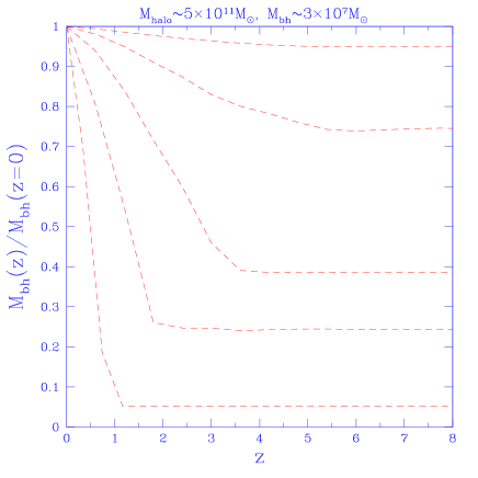
FIG. 1.: Evolution to give the present day black hole in a $5\times 10^{11}M_{\odot}$ halo with redshift for various accretion efficiency factors. From top to bottom the evolutions are for $\epsilon_{acc}=10^{-7},3\times 10^{-7},10^{-6},3\times 10^{-6}$,and $10^{-5}$.

FIG. 2.: Evolution of mass and number density for galactic black holes for 4 different accretion efficiencies. The data points are the inferred mass density values of Chokshi and Turner. The initial mass density and number density of black holes are taken to be $1\times 10^{4}M_{\odot}Mpc^{-3}$ and $4\times 10^{-3}Mpc^{-3}$ at $z=0$ respectively. The number density at early time reaches $9\times 10^{-3}Mpc^{-3}$ at $z=10$ for the scenario that is consistent with observations. As one views the number density evolution from high z, the increase in number density arises from the formation of astrophysical black holes due to halo matter accretion. The contribution of astrophysical black holes becomes more prevalent as the accretion efficiency is increased.

Figure 1 demonstrates, for the case of a single halo, how the accretion efficiency, $\epsilon_{acc}$, in (6) has a strong influence on how much of the black hole mass could be present at higher redshifts. In figure 2 we show the evolution of the total comoving energy and number densities for black holes with redshift. There is an intuitive play off, shown in figure 2, between the accretion efficiency and the fraction of black holes originating at early times. The higher the accretion rate, the higher the chance is of black holes being formed at late times, during the halo merging, as opposed to being primordial. As discussed in [13], constraints can be placed on the efficiency coefficient using inferred accretion rates from QSO luminosity functions [32]. One can see that the QSO evolution data places a tight constraint on the accretion efficiency parameter: for $M_{l}=10^{10}M_{\odot}$ one requires $\epsilon_{acc}\sim 1.85\times 10^{-6}$. In this scenario we see that the vast majority of black holes, using this accretion prescription, are present prior to halo merging.

An alternative scenario extends the galaxies able to support black holes down to dwarf scales. This can be modeled by lowering the mass threshold to $10^{9}M_{\odot}$. Inevitably this will alter the evolutionary profile; accretion in smaller galaxies will be comparatively more efficient under this model as their gravitational well is not as prohibitive. As is shown in figure 3 this leads to a slight reduction in the predicted comoving energy density of black holes at early times. However, the general conclusions are the same in that the PBHs still contribute a significant fraction of the energy density today and comprise the majority of the total number of black holes involved in the evolution.

In figure 4 we provide the main output of this section. We show the expected mass distribution for the primordial black hole for $M_{l}=10^{10}M_{\odot}$ and $M_{l}=10^{9}M_{\odot}$. Their masses, typically $M_{bh}\sim 10^{3}-10^{6}M_{\odot}$, are still many orders of magnitude larger than stellar mass scales, even considering the potential merging of early massive stars. We propose that such black hole masses could be generated through early time accretion of a quintessential scalar field onto PBHs. In the following sections we investigate such a scenario and show that mass distributions such as those is figure 4 can be obtained.

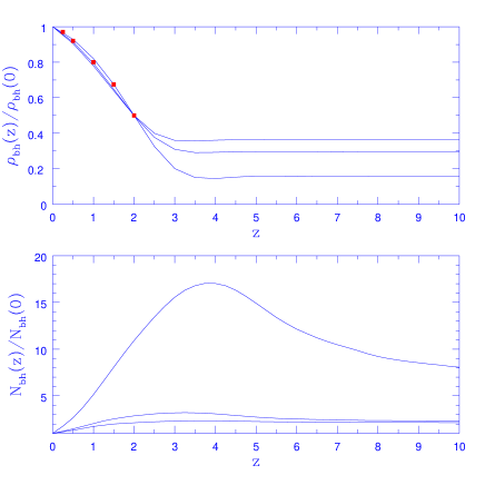
FIG. 3.: Evolution of mass and number density of black holes in galaxy scale halos for 3 different limiting mass thresholds. Reading top to bottom for mass density and bottom to top for number density $M_{l}=10^{10},5\times 10^{9}$ and $10^{9}M_{\odot}$ with accretion efficiencies of $\epsilon_{acc}=1.85,1.63$ and $1.38\times 10^{-6}$ respectively chosen to be in agreement with low z QSO observations

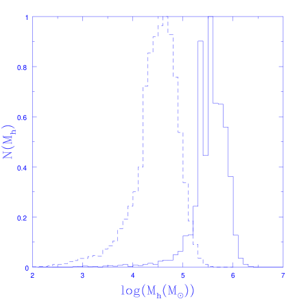
FIG. 4.: Distribution of black hole masses at redshifts preceding halo merger activity for the models in fig 3 with $M_{l}=10^{10}M_{\odot}$ (full line) and $10^{9}M_{\odot}$ (dashed line). The distributions are normalised to their peak values.

III The effects of evaporation and accretion on primordial black holes

There has been intense discourse regarding whether or not PBHs are capable of accreting radiation. Carr and Hawking gave arguments for negligible accretion [19], but these were later disputed (see [20] and references therein). In any case these arguments only apply to perfect fluids and a scalar field $\phi$ is not a perfect fluid (even though an isotropic, homogeneous scalar field does behaves like a perfect fluid). In Appendix 2 we show that even for the simplest potentials $V(\phi)$ the field is indeed absorbed by the black hole leading to a mass increase with rate:

$${dM\over dt}=4\pi(2M)^{2}\dot{\phi}_{c}^{2}$$ (7)

where $\phi_{c}$ is the cosmological solution for $\phi$. For more general potentials it may well be the case that the proportionality constant in the equation receives corrections of order 1, but these shall not matter for the rest of the argument in this paper.

From eqn. 7 we note that kinetic (but not potential) scalar energy leads to black hole growth. This is consistent with the result that the presence of a cosmological constant does not lead to equivalent growth.

Assuming now a potential of the form $V=V_{0}e^{-\lambda\phi}$, we have

$$\phi={2\over\lambda\sqrt{8\pi}}\log{t\over t_{0}}$$ (8)

(using $G=1$, not $8\pi G=1$), leading to:

$${dM\over dt} = \kappa{M^{2}\over t^{2}}$$ (9)

$$\kappa = {8\over\lambda^{2}}$$ (10)

Eqn. 9 integrates to

$${1\over M}={1\over M_{0}}+\kappa{\left({1\over t}-{1\over t_{0}}\right)}$$ (11)

leading to the asymptotic mass:

$$M_{\infty}={M_{0}\over 1-{\kappa M_{0}\over t_{0}}}$$ (12)

for black holes with a mass smaller than a critical mass $M_{crit}=t/\kappa$. These black holes eventually stop accreting and therefore are subdominant with respect to all others. For $M=M_{crit}$ BHs grow like $t$. Above this value the black holes would seem to grow faster that $t$, however clearly the approximations used must break down at this stage. In [20] it was shown that causality constrains these to grow like $t$ as well, a result we shall use for the rest of our calculations.

Hence there is a critical mass at time of formation when PBHs may grow proportionally to the horizon mass. This critical mass separates those black holes which will be of relevance for out scenario and those which won’t.

FIG. 5.: The evolution of black holes ignoring evaporation.

In addition PBHs may experience significant evaporation, via Hawking radiation. This leads to a decrease in their mass, at rate:

$${dM\over dt} = -{\alpha\over M^{2}}$$ (13)

$$\alpha = {\Gamma\over 15360\pi}$$ (14)

This equation can be integrated into

$$M=(M_{0}-3\alpha(t-t_{0}))^{1/3}$$ (15)

implying an evaporation time of

$$\tau={M_{0}^{3}\over 3\alpha}$$ (16)

or

$${\tau\over 10^{17}sec}\approx{\left(M\over 10^{15}g\right)}^{3}$$ (17)

For black holes formed at temperatures much smaller than the Planck temperature this effect can be ignored.

Considering now both accretion and evaporation the black hole mass rate equation becomes

$${dM\over dt}=-{\alpha\over M^{2}}+\kappa{M^{2}\over t^{2}}$$ (18)

which does not have analytical solutions. However, if the temperature at which the black holes are produced is not close to the Planck temperature the interplay of accretion and evaporation is very simple. Black holes with $M_{0}>M_{crit}$ will grow with $M\propto t$, and since their mass was never too small they never experience significant evaporation. Black holes with $M_{0}<M_{crit}$ will stop growing at some $M_{\infty}$, following (11). If this is smaller than $10^{15}g$ they will evaporate before today following (15). Accretion and evaporation happen at very distinct times, so although we do not have an exact solution to (18) it is an excellent approximation simply to glue together back to back (11) and (15).

For reheating temperatures of the order of the Planck temperature the situation is more complicated as evaporation may be significant while black holes are accreting. The result of a numerical integration is plotted in Fig. 6 (to be compared with Fig. 5). We see that the effect of evaporation is then to shift upwards the critical mass $M_{crit}$ above which the black hole mass scales like $t$. In addition, black holes with masses lower than $M_{crit}$ are quickly removed by the effects of evaporation even while they are accreting.

FIG. 6.: The evolution of black holes formed at Planck time with $\alpha=\kappa=1$.

IV PBH formation and their comoving density

Having identified the conditions required from PBHs in terms of early-time accretion and late-time merging, we now proceed to construct a cosmological scenario in which they are satisfied. Although not compulsory, for definiteness we consider an inflationary scenario with a reheating temperature $T_{r}$ and a tilted spectrum of scalar perturbations with a spectral index $n_{s}>1$. The index $n_{s}$ need not be a constant and indeed many inflationary models predict a running tilt, varying from scale to scale. Bearing this in mind we stress that the constraints upon $n_{s}$ discussed in this section refer to very small scales (the horizon size at $T_{r}$), widely different from the scales probed by CMB fluctuations or large scale structure surveys.

As shown in [16] for suitable $n_{s}$ one may have production of PBHs in a short time window immediately after reheating. Typically a black hole is formed if the density contrast on the horizon scale exceeds a given critical value, $\delta>\delta_{c}$. Its mass is given by:

$$M_{bh}=kM_{H}(\delta-\delta_{c})^{1/\gamma}.$$ (19)

Numerical studies with PBHs formed in a pure radiation background have identified $\delta_{c}$, $k$ and $\gamma$ [22, 23]; it may be that quintessence modifies these values slightly however for simplicity we take the calculated values $k=3.3,\gamma=0.34$. But given the uncertainty we consider two values of $\delta_{c}$ in this section $\delta_{c}=0.25,1$. The correct value should be somewhere in between. In section V we assume the value $\delta_{c}=0.67$ to outline a precise example.

Note that the horizon scale is important because it is the relevant Jeans scale for radiation but also for the quintessence field. In Appendix 1 we present a simple model for the formation of PBHs with quintessence: some peculiarities are found, but they should not affect the rest of the argument.

The mass variance on the horizon scale at temperature $T$ is [16]:

$$\sigma_{H}=10^{-4}{\left(10^{-17}{\left({T\over{\rm Mev}}\right)}^{-2}\right)}^{1-n_{s}\over 4}$$ (20)

To a good approximation, as shown in figure 9, we may assume that all PBHs are formed immediately after reheating, since $\sigma_{H}$ then decreases sharply making black holes rarer.

We have seen that we expect no black hole coalescence for redshifts higher than $z\approx 10$. Hence the comoving density of PBHs can be directly related to the probability of an accreting black hole being formed, $p_{acc}$. This is the probability of $\delta>\delta_{crit}$, i.e. the probability for black hole formation and accretion in each horizon.

$$p_{acc}=\int_{\delta_{crit}}^{\infty}{e^{-\delta^{2}\over 2\sigma_{H}^{2}}\over{\sqrt{2}\pi}\sigma_{H}}d\delta\approx{e^{-\delta^{2}_{crit}\over 2\sigma_{H}^{2}}\over 2\pi}$$ (21)

(where the last approximation comes from [33]) and where $\delta_{crit}$ is the value of $\delta$, in equation (19), that would create a black hole of critical mass, $M_{crit}$. The comoving density of accreting black holes is $n\approx p_{acc}/({4\over 3}\pi r_{H}^{3})$ where $r_{H}$ is the comoving horizon radius at $T_{r}$. The latter is given by $r_{H}=2ta_{0}/a\approx 80(T/{\rm Mev})^{-1}Pc$ so that

$$n=4.6\times 10^{11}p_{acc}{\left(T\over{\rm Mev}\right)}^{3}{\rm Mpc}^{-3}$$ (22)

Combining (20), (21) and (22), and to be consistent with Fig. 2, requiring that $n\approx 9\times 10^{-3}{\rm Mpc}^{-3}$ we obtain a value for $n_{s}$ for each value of $T_{r}$. In Fig. 7 we plot the required $n_{s}(T)$ for the two values $\delta_{c}=0.25,1$, using a fixed value of $M_{crit}(\lambda)$. As mentioned above, the correct value of $\delta_{c}$ should lie somewhere in this region. In Fig. 7 we plot the required tilt for three different critical masses with fixed $\delta_{c}=0.67$.

The tilts required fit within the constraints of [34], and can accommodate the recent reionisation tilt constraint of [35] with $n_{s}<1.27$ with a high reheat temperature $>\sim 10^{15}Gev)$.

FIG. 7.: The value of the spectral index $n_{s}$ (on the scale of the horizon at the time of PBH formation) resulting in the correct comoving density for SMBH seeds. The two curves correspond to $\delta_{c}$=0.25,1 and $\lambda=3$ is taken as an example.

FIG. 8.: The value of the spectral index $n_{s}$ (on the scale of the horizon at the time of PBH formation) for three different critical masses relating to $\lambda=2,3,4$. $\delta_{c}$ is fixed =0.67.

Note that the primordial black hole comoving density imposed in our considerations is much smaller than that considered in [16]. Indeed the black holes studied by [16] do not grow (as opposed to ours ). The idea in [16] is to produce a larger density of much lighter black holes, suitable to promote them to candidates for dark matter. Our purpose is to generate a much lower density of much heavier PBHs, so that they could supply the primordial eggs for the merging history of SMBHs.

V The PBH mass spectrum

As an example we calculate the mass spectrum following the methods of [16] to evaluate the initial mass spectrum. This involves using a Monte-Carlo technique to obtain black hole masses which, unfortunately, is computationally unfeasible for low $p_{acc}$ $(\sim<10^{-7})$ required to give the correct comoving densities for $\lambda>2$. With this in mind, we consider two scenarios which provide the correct comoving number density of PBHs ($9\times 10^{-3}Mpc^{-3}$ assuming a limiting mass of $10^{10}M_{\odot}$ in section II), one with a reheat temperature of the order $T_{r}=10^{10}Gev$, tilt $n_{s}=1.33$ and a second with reheat temperature $T_{r}=10^{4}Gev$, $n_{s}=1.57$ with $\lambda=2$ in each case. As Fig. 9 shows most black holes, and in particular those that are able to accrete, are then formed immediately after reheating, with a slight spread in their masses, which we further display in Fig. 10.

FIG. 9.: The demography of black hole formation with a reheat temperature of $T_{r}=10^{10}Gev$ and tilt $n_{s}=1.33$. The crosses represent Monte Carlo simulated black holes. The full and dashed lines are the horizon and critical mass, the latter assumes $\lambda=2$.

FIG. 10.: The bottom panel shows the initial black hole mass distributions for the two scenarios described in the text, with reheat temperatures $(T_{r})$ of $10^{10}Gev$ (dashed line) and $10^{4}Gev$ (full line). The upper panel shows the same distributions comparing them to the critical mass at the time of each black hole’s formation. A blackhole will accrete if $(M_{bh}/M_{crit})>1$. In each panel the distributions are normalised to 1 at their peak for ease of comparison.

We then evolve this initial mass distribution considering accretion and evaporation in a quintessence model as described in Section III. We assume, however, that the quintessence field goes off scaling and kinates at a temperature of the order $T=1Mev$, since if the field continues to scale after this time one ends up with too large masses. Nevertheless if the field goes off scaling the black holes stop accreting (cf. Eqn 7), and even if the field starts scaling subsequently, BHs will not grow significantly again, since their growth pause has rendered them subcritical. Hence in what follows what we need is simply a brief pause in scaling at a temperature of around $T=1Mev$. We shall consider two examples here, one with $T_{off}\approx 4Mev$, and another with $T_{off}=1Mev$.

In Figs. 11 and 12 we find that the projected mass spectra at $z\approx 10$ (or indeed at any time after $T_{off}$ but before the galactic merging history started). In Fig. 11 we plot results for PBHs formed at a reheating temprature of $T_{r}=10^{4}$ Gev as described above. In Fig. 12 we plot the corresponding distribution for the scenarios in which $T_{r}=10^{10}$ Gev. In both cases note that the existence of a critical mass for accretion implies that the final distribution mimicks the initial one clipped at the critical mass. For the first scenario considered the cut off is at the peak of the distribution; hence the final distribution is very skewed. For the second scenario the cut off is to the left of the peak - so the final distribution is more symmetric. As expected if the field goes of scaling later, the final PBH masses are much larger: for $T_{off}=4$ Mev we find final PBH masses of the order of $10^{4}-10^{5}M_{\odot}$; for $T_{off}=1$ Mev these masses grow to $10^{5}-10^{6}M_{\odot}$.

In either case these plots are entirely consistent with those obtained from the merging history in section II (Fig. 4). Quintessence could have therefore provided the primordial seeds which then turn into the SMBHs we observe today.

FIG. 11.: The distribution of black hole masses at redshift $z\approx 10$ for quintessence models deviating from scaling at $T\approx 5Mev$, and $1Mev$ (we have used a reheating temperature of $T_{r}=10^{4}$ Gev and $\lambda=2$). In both cases the distribution is skewed, reflecting the exitence of a critical mass for growth. The later quintessence leaves scaling the larger the BHs’ mass.

FIG. 12.: The distribution of black hole masses at redshift $z\approx 10$ for quintessence models deviating from scaling at $T\approx 5Mev$, and $1Mev$ (we have used a reheating temperature of $T_{r}=10^{10}$ Gev and $\lambda=2$).

VI Conclusions

We have demonstrated that a scenario in which primordial black holes attain super massive size through the accretion of a cosmological scalar field is wholly consistent with current observational constraints. Such a model can generate the correct comoving number density and mass distribution for SMBH’s, given a standard prescription for late-time merging and matter accretion and with reasonable choices of tilt.

Existing schemes explaining SMBHs require very contrived choices of parameters (e.g.[10]). The root of all the evil lies in the huge mass discrepancy between cosmic scale masses (such as those considered in previous studies of PBHs) and those of their supermassive cousins - the cosmological counterpart of the discrepancy between solar mass objects and SMBHs found in astrophysical schemes. We attempt to bridge the mass scale gap in our model by allowing primordial holes to grow by accreting quintessence. Still, we find that we have to switch off this process at a carefully tuned time, so that there is not too much growth.

The fact that this requirement is equivalent to requesting that quintessence goes off scaling just before nucleosynthesis is of some consolation: such a feature is already present in non-minimally coupled quintessence models such as those studied by [39]. In these scenarios the present acceleration of the universe results from a coupling between quintessence and dark matter. It switches on close to the radiation to matter transition, but is affected by a long transient. This explains why the universe did not start accelerating until nowadays. The fact that this transient is symmetric around equality, and that equality is an equal number of expansion times from us and from nucleosynthesis, then makes the field kinate away at nucleosynthesis time.

In addition, in order to obtain the correct comoving density we have to tune carefully the value of the scalar tilt, $n_{s}$, on the scale of the horizon at the time of primordial black hole formation. However this fine tuning is a problem with any theory employing primordial black holes for astrophysical purposes, such as as candidates for dark matter [16], and is no better or worse in our theory.

In spite of these fine tuning problems we believe that this is an interesting scenario which deserves further work. The effects of angular momentum upon the whole picture are perhaps the most important next issue to consider.

Acknowledgements We would like to thank Andrew Jaffe, Lev Kofman, Andrew Liddle, David Spergel and Paul Steinhardt for their helpful thoughts and comments. RB is supported by PPARC.

VII Appendix I - PBH creation and quintessence

In this appendix we the examine the effects of quintessence on PBH formation using the spherical model. The idea is to follow non-linear collapse of a super-Jeans size spherical region by modelling the overdense region as a portion of a Friedmann closed model pasted onto a flat model. Setting up this model entails studying the dynamics of quintessence in closed models. For completeness we shall also consider open models, which may be of relevance for modelling the void structure of out universe.

A Quintessence in open and closed models

The relevant equations are:

$${\left(\dot{a}\over a\right)}^{2} = {1\over 3}{\left(\rho+\frac{1}{2}\dot{\phi}^{2}+V(\phi)\right)}-{K\over a^{2}}$$ (23)

$$\rho+3\displaystyle{\frac{\dot{a}}{a}}(\rho+p) = 0$$ (24)

$$\ddot{\phi}+3\displaystyle{\frac{\dot{a}}{a}}\dot{\phi} = \lambda e^{-\lambda\phi}$$ (25)

where dots represent derivatives with respect to proper time. It is well know that if $K=0$ with $p=w\rho$ we have:

$$a \propto t^{2\over 3(1+w)}$$ (26)

$$\rho \propto {1\over a^{3(1+w)}}$$ (27)

$$w_{\phi} = w$$ (28)

$$\Omega_{\phi} = {\rho_{\phi}\over\rho+\rho_{\phi}}={3\over\lambda^{2}}(1+w)$$ (29)

$$\phi = {2\over\lambda}\log{t\over t_{0}}$$ (30)

We call this solution the scaling solution. With $K\neq 0$ this is also the solution at early times, when curvature is subdominant.

Without quintessence open models ($K=-1$) at late times become vacuum dominated - the so called Milne Universe for which $a\propto t$. However we find that in the presence of quintessence the onset of negative curvature domination leads to another scaling solution: one in which curvature and quintessence remain proportional. We find that:

$$a \propto t$$ (31)

$$\rho_{\phi} \propto {1\over a^{2}}$$ (32)

$$w_{\phi} = -{1\over 3}$$ (33)

$$\Omega_{\phi} = {\rho_{\phi}\over\rho_{c}}={2\over\lambda^{2}}$$ (34)

$$\phi = {2\over\lambda}\log{t\over t_{0}}$$ (35)

which implies that open universes at late times are devoid of normal matter, but not of quintessence. This type of behavior can be understood from the $K=0$ scaling solution, considering that open curvature behaves like a fluid with $w=-1/3$. In the same way that quintessence locks on to matter or radiation in a scaling solution, it locks on to open curvature.

As is well known, without quintessence closed models ($K=1$) expand and eventually turn around and collapse in a Big Crunch. This type of behavior is not changed by the presence of quintessence; however the scaling behavior of quintessence itself is drastically changed. As the universe comes to an halt the friction term in the $\phi$ equations (that is the term $3{\dot{a}\over a}\dot{\phi}$) is withdrawn and the field becomes kinetic energy dominated (i.e. it kinates). Hence as the universe turns around quintessence becomes subdominant, as it scales like $\rho_{\phi}\propto 1/a^{6}$ in contrast with $\rho\propto 1/a^{3}$.

However as the universe enters the contracting phase what used to be a friction term starts to drive the field, since now ${\dot{a}\over a}<0$. This leading to runaway kination, since it is precisely the balance of braking and the slope of $V(\phi)$ what usually moderates the balance of kinetic and potential energy. As before, kinetic energy domination implies $w_{\phi}=1$ and a faster decay rate with expansion $\rho\propto 1/a^{6}$. However contraction reverses the argument, and whatever has stronger dilution rate during expansion, will have higher compression rate during contraction. Therefore, at late stages of collapse quintessence dominates. Since curvature and background matter can be ignored we have the solution:

$$a \propto (t_{c}-t)^{1/3}$$ (36)

$$\rho_{\phi} \propto {1\over a^{6}}$$ (37)

$$w_{\phi} = 1$$ (38)

$$\Omega_{\phi} \approx 1$$ (39)

$$\phi \propto a^{-1/{\sqrt{6}}}$$ (40)

in which $t_{c}$ is the crunch time.

B Implications for structure formation and PBH formation

Qualitatively these results indicate that quintessence has a leading role in the strongly non-linear stages of structure formation. Voids should be filled with quintessence, judging from what happens to the $K=-1$ case. Also it would appear that black hole formation would be led by quintessence and not by matter (as implied by the $K=1$ case). Interestingly, quintessence appears to behave like a stiff fluid ($p_{\phi}=\rho_{\phi}$) during collapse, so we should be able to simplify the calculations. The black hole mass seems to be dominated by the amount of quintessence accreted. Also because $M_{\phi}\propto\rho_{\phi}a^{3}\propto 1/a^{3}$, there must be a mass enhancement during collapse (due to gravity acting against quintessence’s pressure).

All of these effects may at most introduce factors of order 1 in the calculations in the main body of the text, and so interesting as these results might be we have relegated them to Appendix.

VIII Appendix II - Quintessence around a black hole

Given the large Jeans mass of quintessence, its fluctuations should be very small even in the interior of non-linear objects, such as the Solar system. Indeed the relativistic restoration force induced by the $\phi$ gradients should ensure that quintessence fluctuations remain linear, even under highly non-linear gravitational forces. One obvious exception is the vicinity of a BHs horizon, where $\phi$ has to change drastically.

The interaction of BHs and quintessence then becomes a problem of boundary matching: on one side the homogeneous cosmological solution; on the other the infinite radius limit of the Schwarzchild solution. This matter has been examined in the literature in the context of the gravitational memory problem in Brans-Dicke theories [36, 37]. Our analysis will closed mimic that of Jacobson [38].

We assume that the cosmological scalar field generates a much weaker gravitational field than the black hole, so that we can impose a Schwarzchild metric, with a quasi-stationary mass parameter. Hence the equation for the scalar field is the vicinity of the BH is:

$$\Box\phi=-{\ddot{\phi}\over A}+{1\over r^{2}}(r^{2}A\phi^{\prime})^{\prime}={\partial V\over\partial\phi}$$ (41)

where $A(r)=1-2M/r$, and dots and dashes are derivatives with respect to time and $r$ respectively. For free waves ($V=0$) the system separates giving:

$$\phi=e^{-i\omega t}R(r)$$ (42)

with:

$${1\over r^{2}}(r^{2}AR^{\prime})^{\prime}+{\omega^{2}\over A}R=0$$ (43)

or introducing a Kruskal coordinate $r^{\star}$, such that $Adr^{\star}=dr$ (or $r^{\star}=r+2M\log({r\over 2M}-1)$):

$${d^{2}R\over dr^{\star 2}}+{2A\over r}{dR\over dr^{\star}}+\omega^{2}R=0$$ (44)

It is clear that far away the solutions are:

$$\phi={e^{i\omega(t\pm r)}\over r}$$ (45)

and that near the horizon they become:

$$\phi=e^{i\omega(t\pm r^{\star})}$$ (46)

Focusing on solutions regular on the horizon ${\cal H}^{+}$, we introduce the advanced time coordinate $v=t+r^{\star}$, so that the relevant oscillatory solutions take the form $e^{i\omega v}$.

In addition there are non-oscillatory solutions regular at $r=2M$, such as those studied by Jacobson. These can be obtained noting that (41) can be rewritten as:

$$2\phi_{,rv}+{2\over r}\phi_{,v}+{1\over r^{2}}(r^{2}A\phi_{,r})_{,r}=-V^{\prime}(\phi)$$ (47)

For a general $V(\phi)$ separability is lost and numerical work is necessary. In order to further the analytical approach we model the rolling potential by its gradient at a point $V=-\mu\phi$ (we could add a constant here without loss of generality). Equation (47) then becomes:

$$2\phi_{,rv}+{2\over r}\phi_{,v}+{1\over r^{2}}(r^{2}A\phi_{,r})_{,r}=-\mu$$ (48)

Setting $\phi=f(v)+g(r)$ leads to $f=Bv+D$, and

$$g_{,r}={-\mu r^{2}\over 3(r-2M)}-{Br\over r-2M}+{C\over r(r-2M)}$$ (49)

For the solution to be regular at the horizon we must have:

$$C=4M^{2}{\left(B+{2\over 3}\mu M\right)}$$ (50)

Integrating finally leads to:

$$\phi = B[v-r-2M\log r]-$$ (52)

$$-{\mu\over 3}{\left({r^{2}\over 2}+2Mr+4M^{2}\log r\right)}+D$$

which generalized Jacobson’s solution. The general solution is a superposition of free oscillatory solutions and this solution.

We must now impose a boundary condition of the form:

$$\phi=\phi_{c}+\dot{\phi}_{c}t$$ (53)

where $\phi_{c}$ refers to the quintessence cosmological solution. If we fix $B$ and $D$ so that:

$$\phi = \phi_{c}+\dot{\phi}_{c}\left[v-r-2M\log{r\over 2M}\right]-$$ (55)

$$-{\mu\over 3}{\left({r^{2}\over 2}+2Mr+4M^{2}\log{r\over 2M}\right)}$$

we have asymptotically:

$$\phi=\phi_{c}+\dot{\phi}_{c}t-{\mu\over 6}r^{2}$$ (56)

A small error is made in matching the two conditions, but in a quintessence scenario with

$$\mu\approx{\partial V\over\partial\phi}=\lambda V=\lambda\Omega_{\phi}\rho$$ (57)

(where $\lambda$ has units of $1/\phi$ and is expressed in Planck units and $\rho$ is the cosmological density) we find thatthe scale on which the error becomes significant is the cosmological horizon scale. Hence this small error can be neglected.

Computed the flux of energy through the BH horizon associated with this solution:

$${\cal F}=T_{vv}=\dot{\phi}_{c}^{2}$$ (58)

we finally find an equation for the BH mass:

$${dM\over dt}=4\pi(2M)^{2}\phi_{c}^{2}$$ (59)

which is the same formula derived by Jacobson. Hence we conclude that the potential $V(\phi)$ only has indirect impact upon the BH mass, via its effect upon the time evolution of the cosmological solution $\phi_{c}$.

REFERENCES

- [1] J. Kormendy and D. Richstone, ARA& A, 33, 581 (1995).
- [2] D. Richstone et al, Nature 395 A14-A19, 1998.
- [3] D. Richstone, astro-ph/9810379.
- [4] J. Magorrian et al, Astron.J.115: 2285, 1998.
- [5] D. Merritt and L. Ferrarese, astro-ph/0107134.
- [6] R. Van der Marel, Ap J 117, 711 (1999).
- [7] A. J. Barger et al, ApJ, 122, 2177 (2001).
- [8] F. Melia and H Falcke, ARA&A, Vol. 39 (2001).
- [9] J.W. Moffat, astro-ph/9704232.
- [10] J. Hennawi and J. Ostriker, astro-ph/0108203.
- [11] J. Silk and M. J. Rees, astro-ph/9801013.
- [12] A. Cattaneo, M.G. Haehnelt, M.J. Rees, astro-ph/9902223.
- [13] A. Cattaneo, M.G. Haehnelt, M.J.Rees astro-ph/9902223
- [14] K. Gebhardt et al. astro-ph/0006289
- [15] M. Sarzi et al. astro-ph/0110673
- [16] A. M. Green, A. R. Liddle, Phys.Rev. D56: 6166-6174, 1997.
- [17] T. Kanazawa, M. Kawasaki and T. Yanagida, Phys.Lett.B482:174-182,2000
- [18] K. Jedamzik, Phys.Rev.D55:5871-5875,1997.
- [19] B. Carr and S. Hawking, MNRAS 168, 399, 1974.
- [20] E. Bettwieser and W. Glatzel, Astron. and Astrophys. 94, 306, 1981.
- [21] P. Custodio and J. Horvath, Phys.Rev.D58:023504,1998.
- [22] J.C. Niemeyer and K. Jedamzik, Phys. Rev. Lett. 80, 5481 (1998); Phys. Rev. D59, 124013 (1999).
- [23] K. Jedamzik and J.C. Niemeyer, Phys. Rev. D59, 124014 (1999).
- [24] C Wetterich, Nucl. Phys B. 302 668 (1988)
- [25] B. Ratra and J. Peebles, Phys. Rev D37 (1988) 321.
- [26] J. Frieman, C. Hill, A. Stebbins, I. Waga, Phys. Rev. Lett, 75 2077 (1995).
- [27] I. Zlatev, L. Wang, & P. Steinhardt, Phys. Rev. Lett. 82 896-899 (1999).
- [28] A. Albrecht & C. Skordis, Phys. Rev. Lett. 84, 2076-2079 (2000).
- [29] C. Lacey, S. Cole MNRAS 262 (1993) 627
- [30] R.S. Somerville, T.S. Kolatt astro-ph/9711080
- [31] W.H. Press, P. Schechter ApJ 187 (1974) 425
- [32] A. Chokski, E.L. Turner MNRAS 259 (1992) 421.
- [33] Gradshtein and Ryznikp, ***, pp 939.
- [34] A. R. Liddle and A. Green, Phys.Rept. 307 (1998) 125-131
- [35] Ping He and Li-Zhi Fang, astro-ph/0202218 (2002)
- [36] J. Barrow, Phys. Rev. D 46, R3227 (1992).
- [37] J. Barrow and B. Carr, Phys. Rev. D54, 3920 (1996)
- [38] T. Jacobson, Phys. Rev. Lett. 83, 2699, (1999).
- [39] R. Bean and J. Magueijo, Phys.Lett. B517, 177, (2001).