Velocity Fields of Disk Galaxies
Abstract
Two dimensional velocity fields have been an important tool for nearly 30 years and are instrumental in understanding galactic mass distributions and deviations from an ideal galactic disk. Recently a number of new instruments have started to produce more detailed velocity fields of the disks and nuclear regions of galaxies. This paper summarizes some of the underlying techniques for constructing velocity fields and deriving rotation curves. It also urges to simulate observations from the data-cube stage to reject subtle biases in derived quantities such as rotation curves.
Astronomy Department, University of Maryland, College Park, MD 20742, USA
1. Introduction
Two dimensional radial velocity fields of galactic disks are now routinely derived from an ever increasing number of optical and radio emission and absorption lines (HI, CO, H, [NII], …) using a variety of instruments (Radio and Fabry-Perot interferometers, integral field spectrographs (IFS)). These data are normally obtained as three dimensional data-cubes, from which by either fitting some functional form to the spectral line, or a moment analysis, a velocity field is derived. Such two dimensional velocity fields are then fitted with a rotation curve by assuming circular rotation (Begeman 1989). Analysis of rotation curves and comparison with models and observations have led to the realization that dark matter in the outer parts of galaxies must be the dominant gravitational force. In addition the question of the contribution of the stellar disk to that of the dark matter (van Albada & Sancisi 1986) and the validity of Cold Dark Matter (de Blok et al. 2002) are both derived from simple 1-dimensional rotation curves. The process of deriving a 1-dimensional rotation curves from a 3-dimensional data-cube is subject to many observational, instrumental and physical biases, which we review here. Older reviews range from the classic van der Kruit & Allen (1978) paper to last year’s review by Sofue & Rubin (2001). A number of (often Dutch111may contain a slight author bias) PhD. theses also discuss many basic aspects (Bosma 1978, Begeman 1987, Broeils 1992, de Blok 1997, Swaters 1999, Wong 2000) and although sometimes hard to retrieve, are worth reading. In this paper we will start from rotation curves, construct velocity fields, and conclude by looking at how velocity fields are constructed from data cubes.
2. Rotating Galactic Disks
Our ideal mathematical galactic disk is infinitesimally thin, and has material rotating on circular orbits of negligible velocity dispersion. Inclined at an angle to the sky plane, and a major axis aligned with the axis for convenience, the observed radial velocity is given by
| (1) |
where are polar coordinates measured in the plane of the galaxy, and the cartesian coordinates on the plane of the sky. By convention, position angles are measured counter clockwise from the receding side, , of the galaxy major axis. For later discussions we add an expansion term, ; for circular orbits this term will be 0 of course.

The relationship between the sky and galaxy plane is given by:
| (2) |
2.1. Linear rotation curve (solid body)
The centers of galaxies have often been assumed to have a solid body (density ) rotation curve222Any steeper sloped density will have a rotation curve with infinite slope at the center, but beam smearing will generally produce a linear rotation curve.
| (3) |
for which the velocity field (eq. (1)) is given by
| (4) |
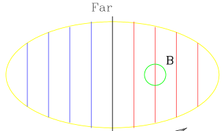
which means equi-velocity contours are lines parallel to the axis (see Fig. 2a) For beam size and tracer velocity dispersion the observed velocity dispersion will be
| (5) |
but note that the mean velocity will not be affected by beam smearing (assuming uniform surface density).
2.2. Flat rotation curve (isothermal body)
In the case of a flat rotation curve (density )
| (6) |
the velocity field is given by
| (7) |
which means equi-velocity contours are now radial lines going through the center (see Fig. 2b). All along the major axis () the maximum amplitude is observed, and any beam smearing will now only include material with lower radial velocities, and thus introduce a bias against the maximum rotation speed. For a beam size this lowest observed radial velocity is approximately given by
| (8) |
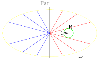
An interesting property of velocity fields of projected circular orbits is that the kinematic major and minor axis, i.e. the lines and maximum velocity gradient are perpendicular to each other, and these are also aligned with the morphological major and minor axis. See also Figure 2.
2.3. Deviations from the Ideal Galactic Disk
Here is a list of some of the known deviations from an ideal galactic disk:
-
•
The disk is not flat. For example warps (e.g. Bosma 1981) or corrugations (Edelsohn & Elmegreen 1997) are known forms of deviations from perfectly flat disks. For warps the velocity field in each annulus is still that of circular orbits, ignoring any precession of the warp.
-
•
The disk is lopsided (m=1 mode) and will not support circular orbits (see e.g. Noordermeer et al. 2002).
-
•
The disk is not axisymmetric (e.g. m=2 mode) and thus non-circular orbits ( orbits in bars, oval distortions, as well as non-spherical dark halos) will be present. Best known examples are barred galaxies, where deviations can easily reach 50-150 km/s (see e.g. Regan, Sheth, & Vogel 1999).
-
•
Disks have spiral arms, i.e an m=2 mode with changing position angle. Deviations from circular orbits can easily reach 10-50 km/s. Spiral arms can also have associated features, such as spurs, that cause higher order harmonics to be present in the velocity field. Recent simulations of spurs seem to create deviations or order 5 km/s (Kim & Ostriker 2002).
-
•
Disks have a finite thickness, and are known to become flaring in the outer parts. This will be important at high inclinations and near the center where integrations along the line of sight become long. They will widen the emission line profiles, but do not necessarily remain Gaussian. See also Olling & Merrifield (2000).
-
•
There can be radial outflows or inflows, often implied in the centers of galaxies (but see also Fraternali et al. 2001, Schinnerer et al. 2000).
-
•
Turbulence in the ISM will add a mostly Gaussian component to the line profiles.
-
•
Asymmetric drift corrections, when random motions provide significant dynamical support (cf. Meurer et al. 1996) will need to be applied to derive the correct dynamically derived mass distribution:
(9) -
•
Beam smearing, especially with high inclinations, will generally result in non-Gaussian profiles. Effects on the rotation curve can be 10-50 km/s if not corrected.
-
•
If the tracer is not uniformly distributed across the beam, there will obviously be a bias in the derived velocity. This is especially important where large velocity gradients are present, such as near the galactic center (see also Figure 6). This will also give non-Gaussian profiles.
-
•
The bulge or nuclear potential can cause warps in the inner parts (see e.g. Schinnerer et al. 2000, where non-circular streaming also appears to be present)
-
•
If the tracer is not optically thin, or if there is dust along the line of sight, velocities will come out skewed. For given model distributions, reasonable corrections can be made (see e.g. Baes & DeJonghe 2001). For disk galaxies this effect can be particularly important in the centers of galaxies, and in highly inclined galaxies.
2.4. Elliptical orbits
To first order elliptical orbits will have a tangential and radial velocity
| (10) |
with for orbits oriented perpendicular to the major axis, and for orbits oriented along the major axis. Combining (1) and (10) then gives:
| (11) |
which is a signature of normal circular orbits. In such degenerate cases it is not possible to detect elliptical streaming (see also Long 1991), but will show either a larger or lower rotation curve, depending on the orientation of the “bar” w.r.t. the galaxy major axis.
The more general case, with an ellipticity at an arbitrary angle
| (12) |
will result in a velocity field in which the kinematic major and minor axis are not perpendicular anymore. Realistic orbits (and gas flow) deviates considerably from simple ellipses (Athannassoula 1992), but the general picture remains.
A Fourier analysis of the observed velocity field (see e.g. Teuben 1991, Schoenmakers et al. 1997)
| (13) |
has also led to considerable insight in velocity fields of non-axisymmetric potentials. Spectral analysis of periodic orbits (Binney & Spergel, 1982) provides a natural translation from the periodic orbits to the Fourier components of the velocity field.
A simple inversion from a velocity field to a mass model for non-axisymmetric mass distributions does not exist yet. Sanders & Tubbs (1980) approached this by searching for a least squares solution between the observed and model gas flow velocity field, and used this to find the best parameterized barred galaxy model description for NGC 5383. Weiner et al. (2001) used this approach to break the degeneracy that normally exists in decomposing an observed rotation curve into a dark matter and an M/L converted disk component (“maximum disk hypothesis”).
3. Rotation Curve: velocity field fitting
To derive a rotation curve from a velocity field, various approaches are possible: Especially if the disk is suspected to have a warp, the disk is divided in annuli, within which the rotation speed and geometrical parameters can be fitted (see e.g. Begeman 1987). One can also keep the geometry for the whole disk fixed, and fit a single shape to the rotation curve (see e.g. van Moorsel & Wells 1985). This will generally result in a better geometric definition of the disk, but residual velocity fields should still be investigated to confirm the absence of any systematic effects. Notable problems are due to the product of in eq.(1), which makes it impossible to determine a kinematic inclination for linear rotation curves, and very hard for low values of the inclination.
The rotcur program in GIPSY/NEMO fits the following function
| (14) |
with now in full glory:
| (15) |
and
| (16) |
for each ring. For circular orbits there are 6 free parameters to each ring: systemic velocity , rotation velocity , inclination , position angle of the receding side of the galaxy , and rotation center , and . Alternatively an expansion velocity, , term can be added to eq.(13), increasing the number of free parameters of this non-linear fit to 7. Also note although each ring is fit and provide just a convenient geometrical description, this has not included any real dynamical effects, such as precession, of those rings in a true warped galaxy. For elliptical streaming a phase shifted component (cf. equation (11)) is added to and , causing and harmonics in the radial velocity field. Attempting a tilted ring fit will take care of the harmonic, leaving a characteristic residual (see e.g. Teuben (1991) Figure 3).
79 306 560 654]teuben_fig3.ps
Although these methods have been applied to numerous galaxies, observed in the HI, H and CO lines, recent integral field spectographs are revolutionizing this field because of their high signal-to-noise. Kinematic inclinations can be reliably measured as low as (see e.g. contributions by Andersen & Bershady in this volume). Non-circular motions (bars, spiral arms) now become the limiting factor in deriving geometric parameters from a velocity field, making it possible to test subtle differences in models.
The tilted-ring fit has 6 free parameters per ring, which makes finding a unique solution hard. In practice one often takes a number of steps to bring the number of parameters down. For example, one determines the center (, , and ) either from a number of broad rings where , are kept fixed at reasonable values (e.g. from optical or IR photometry). Alternatively, since the velocity field near the center can often be assumed to be that of a linear rotation curve, one can also determine from a least squares planar fit to where now the galactic center is determined from optical or IR photometry. Both methods should be compared, to exclude systematic effects such as modes (cf. Beauvais & Bothun 1999, 2001).
Next one fixes , , and , and fits , , and in a number of broad rings. The position angle is usually well determined, whereas the scatter in inclination can be large (Begeman 1989). If there is a clear trend in position angle and/or inclination, a kinematic warp may be present and may have to be corrected for (though elliptical orbits can also mimic a changing inclination, as well as interesting effects such as shown in Figure 4 and 5).
Additionally one can also fix , and just fit and , again in a small number of broad rings. This should bring down the error in , and a weighted average should result in a a good value for the inclination.
Finally, after having checked for kinematic warping, one fixes (or trends) all geometric parameters and just fits for in smaller rings, ideally the width of a beam and interlacing the radii of the rings by half a beam width to obtain a reasonably sampled rotation curve.
4. Data Analysis
The most common technique to derive a velocity field from a data cube is a pixel-based profile analysis. Depending on the data quality and type of observations, a number of different techniques have been employed:
-
•
single gaussian (or Voigt) fit. Works well for good signal-to-noise data, and can also easily be extended when multiple components are present.
-
•
intensity averaged (“mean”) velocity, useful for low signal-to-noise data.
-
•
median velocity, a more robust alternative to mean velocity.
-
•
peak (or peak fit) velocity.
-
•
window (converging mean algorithm, see Bosma 1978)
-
•
largest velocity from a multiple component gaussian fit (Begeman 1989)
-
•
envelope tracing (Sofue & Rubin 2001)
-
•
Gaussian-Hermite moments (van der Marel & Franx 1993)
-
•
Fourier Quotient (Bender 1990)
When the bandwidth of the observations is large compared to that of the spectral line, and to limit the influence of noise, most of these techniques benefit by applying some kind a mask over the data where emission is believed to be present. This can be most effectively done by using a highly spatially (and perhaps spectrally) convolved datacube where the signal-to-noise is higher and defining the mask based on a simple cutoff value in this convolved cube. Iterative schemes which result in maps with varying degree of spatial resolution are also possible, but care has to be given that the new data is not just convolved data from already observed neighboring points (Vogel et al. 1993).
For low signal-to-noise data one can also use the fact that emission is on a “wiggly sheet” in the data cube, and interactively define emission in a set of position-velocity diagrams. Although subjective and labor intensive, this last resort can significantly improve the velocity field. An additional aid can be setting a liberal masking window in velocity space around the expected radial velocity on an earlier iteration on the rotation curve.


For highly inclined galaxies (of which our own Galaxy is a special case) some type of envelope tracing technique has been successful in retrieving a rotation curve (Sofue & Rubin 2001, see also Shane & Bieger-Smith 1966). If the ISM can be resolved, such as is the case in our galaxy, a gaussian decomposition selecting the highest velocity component can also be a successful method. Kregel (2002) recently introduces the “union peel” method for edge-on galaxies.
A full cube fit is the final resort when various geometric and beam smearing effects all take too much effect. An input model then predicts the resulting datacube and iteratively corrections are made to the model until the observational cube matches the theoretical one (e.g. Swaters 1999)
4.1. Modeling
With current computing powers detailed simulations of the observations show (Teuben et al., in prep.) that a datacube can have subtle biases, which in turn adds a bias to the velocity field, which will then result in a biased rotation curve! Consider the case of an interferometric observation of a typical galactic disk. Channel maps around the systemic velocity have features aligned along the minor axis, whereas near both of the extreme velocity channels tend to have features predominantly aligned along the major axis. Depending on such details as the distribution of visibilities in the -plane and adding short spacings to the visibilities, deconvolution will result in differently recovered features in these channel maps. This is illustrated in Figure 4 for a model and simulated velocity field. The input model consisted of a gaussian disk with a FWHM size of 50′′ with a linearly rising rotation curve to ′′ and km/s, and flat at larger radii. A single track with 10 antennae in the BIMA C-array has been used to simulate the observation of this model disk. After mapping and (CLEAN) deconvolution, an “observed” velocity field was constructed by computing an intensity weighted mean velocity by clipping signal above the noise level. After this rotcur was used to retrieve the rotation curve, and geometric parameters. Only the systemic velocity and rotation center were fixed, whereas the remaining 3 parameters were fitted. Figure 5 shows the derived parameters from such a tilted ring fit. Notice that the position angle has been underestimated, and that the disk appears to be slightly warped in nature.
40 170 570 700]teuben_fig5.ps
4.2. Smoothing
For a non-uniform distribution of material across the beam, there can be a bias of the derived velocity, independent of the methodology. Figure 6 shows some of this effect by measuring the gradient of a solid body rotation curve and comparing it to the input value. For decreasing density distributions the velocity will be biased to lower values and thus decrease the measured velocity gradient.
30 160 570 430]teuben_fig6.ps
5. Conclusions
Velocity fields of disk galaxies hardly ever show that of a perfectly rotating disk with circular orbits. Many deviations have been identified, and can be readily derived by studying residual velocity fields. We have also shown some of the complexities that are involved when extracting 1-dimensional rotation curves from 3-dimensional datacubes. In extreme cases care has to be given to model the observations, as they may introduce subtle biases in the process of determining velocity fields and derived parameters.
Acknowledgments.
I wish to thank the Guillermo Haro program for a scientifically stimulating and socially pleasant atmosphere during the workshop and conference, and Rosario Sanchez for keeping my cough under control. I also wish to thank the BIMA SONG team for discussions and fabulous data. Marc Verheijen is acknowledged for discussions around their IFS results. This research was supported by NSF grant AST-9981289.
References
Athannassoula, E. 1992, MNRAS, 259, 328
Baes, M., & Dejonghe, H. 2001, ApJ, 563, L19
Beauvais, C., & Bothun, G. 1999, ApJS, 125, 99
Beauvais, C., & Bothun, G. 2001, ApJS, 136, 41
Begeman, K.G. 1987, PhD. Thesis, University of Groningen.
Begeman, K.G. 1989, A&A, 223, 47
Bender, R. 1990, A&A, 229, 441
Binney, J., & Spergel, D. 1982, ApJ, 252 308
de Blok, W.J.G. 1997, PhD. Thesis, University of Groningen.
de Blok, W.J.G., McGaugh, S.S, & Rubin, V.C. 2002, AJ, accepted (astro-ph/0107366)
Bosma, A. 1978, PhD. Thesis, University of Groningen.
Bosma, A. 1981, AJ, 86, 1791
Broeils, A.H. 1992, PhD. Thesis, University of Groningen.
Edelsohn, D. J., & Elmegreen, B. G. 1997, MNRAS, 287, 947
Fraternali, F., Oosterloo, T., Sancisi, R., & van Moorsel, G. 2001 ApJ, 562, L47
Kim, W.T., & Ostriker, E. 2002, ApJ, (Submitted)
Kregel, M. 2002 (in preparation)
Long, K. 1991, PhD Thesis Princeton University.
Meurer, G.R., Carignan, C., Beaulieu, S.F. & Freeman, K.C. 1996, AJ, 111, 1551
Noordermeer, E., Sparke, L.S., & Levine, S.E. 2002, astro-ph/0112305
Olling, R.P., & Merrifield, M.R. 2000, MNRAS, 311, 361
Regan, M.W., Sheth, K., & Vogel, S.N. 1999, ApJ, 526, 97
Sanders, R.H., & Tubbs, A.D. 1980, ApJ, 235, 803
Schinnerer, E., Eckart, A., Tacconi, L.J., & Genzel, R. 2000, ApJ, 533, 850
Schoenmakers, R.H.M., Franx, M., & de Zeeuw, P.T. 1997, MNRAS, 292, 349
Shane, W.W., & Bieger-Smith, G.P. 1966, B.A.N. 18, 263
Sofue, Y. & Rubin, V. 2001, A&A Rev., 39, 137
Swaters, R.A. 1999, PhD Thesis, University of Groningen
Teuben, P.J. 1991, in Warped Disks and Inclined Rings around Galaxies, ed. S.Casertano, P.Sackett and F.Briggs, Cambridge University Press, 40
van Albada, T.S., & Sancisi, R. 1986, Philos. Trans. R. Soc. London A, 320, 447
van der Kruit, P.C., & Allen, R.J. 1978, A&A Rev., 16, 103
van der Marel, R.P., & Franx, M. 1993, ApJ, 407, 525
van Moorsel, G.A., & Wells, D.C. 1985, AJ, 90, 1038
Vogel, S.N., Rand, R.J., Gruendl, R.A., & Teuben, P.J. 1993, PASP, 105, 666
Weiner, B.J., Sellwood, J.A., & Williams, T.B. 2001, ApJ, 546, 931
Wong, T. 2000, PhD Thesis, Berkeley (Appendix A)