Quantification of Uncertainty in the Measurement of
Magnetic Fields in Clusters of Galaxies

Abstract

We assess the principal statistical and physical uncertainties associated with the determination of magnetic field strengths in clusters of galaxies from measurements of Faraday rotation (FR) and Compton-synchrotron emissions. In the former case a basic limitation is noted, that the relative uncertainty in the estimation of the mean-squared FR will generally be at least one third. Even greater uncertainty stems from the crucial dependence of the Faraday-deduced field on the coherence length scale characterizing its random orientation; we further elaborate this dependence, and argue that previous estimates of the field are likely to be too high by a factor of a few. Lack of detailed spatial information on the radio emission—and the recently deduced nonthermal X-ray emission in four clusters—has led to an underestimation of the mean value of the field in cluster cores. We conclude therefore that it is premature to draw definite quantitative conclusions from the previously-claimed seemingly-discrepant values of the field determined by these two methods.

1 Introduction

Spectral and imaging observations of clusters of galaxies with the XMM and Chandra satellites at energies $\epsilon\leq 10$ keV, are currently yielding detailed information on the thermal properties of the hot intracluster (IC) gas. The improved determinations of gas temperature, density, and metal abundances will greatly improve our knowledge of the intrinsic properties (e.g.,  total mass) of clusters, and will significantly advance the use of clusters as more valued cosmological probes (e.g.,  for the measurement of the Hubble constant, $H_{0}$). However, as has been the case in galaxies, in clusters too a more complete description of the astrophysics of these systems necessitates knowledge of basic nonthermal (NT) quantities such as magnetic fields, and the properties of relativistic electrons and protons.

Direct evidence for the presence of relativistic electrons and magnetic fields in clusters comes from measurements of extended regions of radio (in the frequency range $\sim 0.04-4$ GHz) synchrotron emission in $\sim 30$ clusters (see Giovannini et al.  1999, Giovannini et al.  2000, and references therein). In many of the clusters the emitting region is central, with a typical size of $\sim 1-3$ Mpc. Values of the mean magnetic field and relativistic electron energy densities can be obtained if an assumption is made concerning the relative energy densities in the particles and field. Mean field values of a few $\mu$G have been obtained under the assumption of global energy equipartition. Magnetic fields have also been deduced from the measurement of FR of the plane of polarization of distant radio sources seen through clusters (e.g.,  Kim et al.  1991). The observed drop in the absolute value of the RM over a typical cluster-centric distance of $\sim 0.5$ Mpc provides a statistical measure of the mean field along the line of sight to the radio source. Specifically, in a recent survey of radio sources seen through the cores of 16 clusters, Clarke, Kronberg, and Böhringer (2001, hereafter CKB) have deduced a mean field value of $\sim 5-10\,(\ell/10\ {\rm kpc})^{-1/2}$ $\mu$G, where $\ell$ is a characteristic field spatial coherence (reversal) length.

An important recent development is the apparent detection of NT X-ray emission in four clusters, namely Coma, A2199, A2256, and A2319, by the RXTE (Coma cluster: Rephaeli, Gruber, & Blanco 1999, hereafter RGB; A2319: Gruber & Rephaeli 2001) and by the BeppoSAX (Coma: Fusco-Femiano et al.  1999; A2256: Fusco-Femiano et al.  2000; A2199: Kaastra et al.  2000) satellites. The most likely origin of NT X-ray emission in clusters is Compton scattering of relativistic electrons by the cosmic microwave background (CMB) radiation (Rephaeli 1979). The radio and NT X-ray emissions in three of these clusters are likely to be related, providing considerable motivation for their combined analysis. If so, then the mean value of the magnetic field and relativistic electron density can be extracted based directly on observables—the radio synchrotron and Compton-produced fluxes and the joint power law index. Of the four clusters, the best studied is Coma, for which both RGB and Fusco-Femiano et al.  (1999) determine a mean field value of $\sim 0.2$ $\mu$G.

Emission by NT electrons may possibly be detected also at lower energies: EUV observations of several clusters have reportedly led to the measurement of diffuse low-energy ($65-245$ eV) emission which is possibly NT (Sarazin & Lieu 1998, Bowyer & Berghofer 1998). However, Bowyer et al.  (1999) argue that this emission has been unequivocally detected only in the Coma cluster. The origin of the EUV emission is uncertain; suggestions range from NT bremsstrahlung by a population of energetic (or ‘suprathermal’) electrons which is separate from the radio-emitting relativistic   electrons) (e.g., , Sarazin & Kempner 2000), to Compton scattering of the CMB by lower energy relativistic   electrons (Ensslin, Lieu & Biermann 1999). Because of the very substantial uncertainties regarding the nature and origin of the observed EUV emission, we consider here only the relativistic   electron population that is directly deduced from radio and possibly also NT X-ray emission.

Magnetic field values from Compton-synchrotron, $B_{rx}$, or FR, $B_{fr}$, observations clearly involve very different spatial averages not only of the field itself, but also of the relativistic electron density, or the gas density, along the line of sight, respectively. Whereas $B_{rx}$ is based on a volume average of the magnitude of the field over typical radial regions of $\sim 1$ Mpc, $B_{fr}$ is a weighted average of the field vector and gas density along the line of sight. Generally, therefore, it is not expected that these two measures of the field yield similar values. Indeed, it has already been shown that $B_{rx}$ is typically expected to be smaller than $B_{fr}$ (Goldshmidt & Rephaeli 1993). Moreover, the full expression for $B_{rx}$ includes a ratio of spatial factors (Rephaeli 1979) which are essentially volume integrations over the spatial profiles of the relativistic electrons and field. For lack of spatial information on these profiles, this ratio has been taken to be unity in the analyses of RXTE and BeppoSAX data, resulting in a systematically lower value of $B_{rx}$. Generally, FR observations yielded only a measure of the average field over a sample of clusters; this makes a comparison between $B_{fr}$ and $B_{rx}$ somewhat uncertain. Such a comparison is more meaningful in the case of the Coma cluster, for which there are specific measurements of both $B_{fr}$ (Kim et al.  1990, Feretti et al.  1995) and $B_{rx}$ (RGB, Fusco-Femiano et al.  1999), i.e., A400 and A2634 (Eilek & Owen 2001).

Evidently, the interpretation of cluster Compton-synchrotron and FR observations is not straightforward, particularly with regard to the measurement of the strength of IC fields. In addition to observational errors, there are substantial uncertainties stemming from physical as well as statistical considerations whose effects have never been fully investigated. In view of current and near-future observational capabilities, a systematic study of all the relevant issues is both desirable and timely, and the main objective of this paper.

Large uncertainties in the interpretation of FR, radio synchrotron, and Compton emissions stem from the small number of background radio sources (for FR measurements), and poor (radio) or no (X-ray) spatial information on the distribution of NT emission. The main cause of error is the likely complex morphology of IC magnetic fields and the energetic electron density distribution. The fields are quite likely turbulent, polarized over a range of coherence scales ($\sim 1-50$ kpc), and with large scale ($>100$ kpc) variation of their mean strength. Additional sources of uncertainty are due to the small number of bright radio sources behind galaxy clusters that can serve as probes along their respective lines of sight for estimating polarization effects due to the magnetic field. While increased detector sensitivity and imaging capability at high ($>20$ keV) X-ray energies will help mitigate these limitations, we shall show that prevailing methodologies—despite great efforts to minimize instrument error—remain incapable of reducing the uncertainty in the magnetic fields, and that these uncertainties could be very substantial indeed. The influence of embedded, extended sources requires the development of a more complex model which introduces their influence upon the surrounding IC medium and field environment; this will be the subject of a future paper.

In the following section, we focus on statistical aspects emerging from the determination of the FR measure in the ideal situation wherein the IC medium and its magnetic field are both homogeneous in character. We first show that there is a basic statistical limitation in our ability to measure the mean-squared excess FR in clusters. Next, we explore—in the spirit of Goldshmidt & Rephaeli (1993)—the role of inhomogeneity and turbulent field structure and how they are manifested in observations of FR. Then, we briefly examine how the differing spatial distributions of relativistic particles and fields can affect our inference of field values. In the Discussion we assess the overall quantitative measure of uncertainty in estimating field strengths in clusters, and briefly consider some of its consequences.

2 Statistical Issues in the Measurement of Faraday Rotation

Theoretical research (Crusius-Wätzel et al.  1990, Goldshmidt & Rephaeli 1993) dealing with the FR measure has focused on the random nature of the rotation angle $\chi$ defined by

$$\chi=c_{1}\lambda^{2}\int_{0}^{s}{\rm d}s\,n_{t}\left(s\right)\,B_{\parallel}\left(s\right)$$ (1)

where $c_{1}=0.81$ if $\chi$ is measured in radians and $n_{t}$—the thermal electron density—in $\rm cm^{-3}$; $B_{\parallel}$ is the random magnetic field component in $\mu$G along the line-of-sight, and $s$ is the path length in parsecs. Since $n_{t}\,B_{\parallel}$ behaves as a random variable, the Central Limit Theorem (Feller 1968) and its generalization, known as the Feller-Lindberg Theorem, apply and assure that the outcome is well-approximated by a Gaussian with zero-mean . We have verified that the data presented by CKB, namely column 5 of their Table 1, are Gaussian distributed.

Crusius-Wätzel et al.   (1990) and Goldshmidt & Rephaeli (1993) suggested that the mean-squared fluctuation of the rotation angle be employed instead, namely

$$\left\langle\chi^{2}\right\rangle=c_{1}^{2}\lambda^{4}\int_{0}^{s}\int_{0}^{s}{\rm d}s^{\prime}{\rm d}s^{\prime\prime}n_{t}\left(s^{\prime}\right)n_{t}\left(s^{\prime\prime}\right)\left\langle B_{\parallel}\left(s^{\prime}\right)B_{\parallel}\left(s^{\prime\prime}\right)\right\rangle$$ (2)

where the mean of the rotation angle is presumed to vanish, i.e., $\left\langle\chi\right\rangle=0$, and where $\left\langle...\right\rangle$ denotes the expectation value operator. In observational work by CKB that explored the statistical nature of estimates of $\chi$, they presented data from 16 clusters of galaxies that were assumed to have similar morphologies, and analyzed the emission from 27 radio sources from which FR could be derived. Of the 27 sources projected in the 16 clusters in their sample, 15 are embedded (Clarke, personal communication) cluster members, a fact that complicates the interpretation of their results. (We explore possible ramifications of this in the Discussion.) However, we will use the CKB sample as though it contained only background point sources, such as quasars, as an observational basis for comparison with our Monte Carlo investigations. A basic result from the work of CKB is the confirmation of the role of spatial inhomogeneity. In particular, they observed a clear excess FR in radio sources viewed through the magnetized IC gas as compared to those viewed beyond the main gaseous region of the cluster. However, no specific information on the role of spatial inhomogeneity resulted from their statistical study, an issue addressed theoretically by Goldshmidt & Rephaeli (1993). Indeed, an outstanding issue is how the position of the background source relative to the center of the cluster, what CKB call the “impact parameter”, influences the excess FR.

Since many researchers have invested substantial effort in the determination of the excess FR, we address the statistical significance of the estimates that can be derived from such studies. Suppose that we have $N$ estimates of the Faraday rotation angle $\chi_{i},\,i=1,...,N$, such that the related impact parameters are sufficiently close to each other, so that spatial considerations are less important. In other words, can we use multiple estimates of the excess FR—from roughly equivalent spatial locations and for similar cluster types—to estimate the mean-squared rotation angle, as defined by Crusius-Wätzel et al.  (1990) and by Goldshmidt & Rephaeli (1993). In particular, can we quantify the uncertainties that emerge solely from statistical considerations in such estimates of field strengths? This quantification has never before been done in this context.

We begin by defining an “estimator” of the mean-squared excess Faraday rotation angle $\cal E$, namely the arithmetic average

$${\cal E}={1\over N}\sum_{i=1}^{N}\chi_{i}^{2}\quad.$$ (3)

Since we have assumed a statistically homogeneous sample, we will assume for $i=1,...,N$ that

$$\left\langle\chi_{i}\right\rangle = 0$$ (4)

$$\left\langle\chi_{i}^{2}\right\rangle = \sigma^{2}$$ (5)

where $\sigma^{2}$ defines the variance of the process. Further, we invoke the Central Limit Theorem and the Feller-Lindberg Theorem (as noted above) so that $\chi$ can be assumed to be Gaussian distributed or ${\cal N}\left(0,\sigma^{2}\right)$. Accordingly, we find that

$$\left\langle{\cal E}\right\rangle={1\over N}\sum_{i=1}^{N}\left\langle\chi_{i}^{2}\right\rangle=\sigma^{2}\quad.$$ (6)

As an error estimate for this process, we define the mean squared variation in the estimator $\cal E$ according to

$$\left\langle\left({\cal E}-\sigma^{2}\right)^{2}\right\rangle=\left\langle{\cal E}^{2}\right\rangle-\sigma^{4}=\left\langle{1\over N^{2}}\sum_{i,j=1}^{N}\chi_{i}^{2}\chi_{j}^{2}\right\rangle-\sigma^{4}\quad.$$ (7)

Taking this further, we find that

$$\left\langle\left({\cal E}-\sigma^{2}\right)^{2}\right\rangle = {1\over N^{2}}\sum_{i=1}^{N}\left\langle\chi_{i}^{4}\right\rangle+{1\over N^{2}}\sum_{i\neq j}^{N}\left\langle\chi_{i}^{2}\chi_{j}^{2}\right\rangle-\sigma^{4}$$ (8)

$$= {3\sigma^{4}\over N}+{N-1\over N}\sigma^{4}-\sigma^{4}$$ (9)

$$= {2\over N}\sigma^{4}\quad.$$ (10)

Therefore, we conclude that the RMS uncertainty in this estimator of the excess FR

$$\left\langle\left({\cal E}-\sigma^{2}\right)^{2}\right\rangle^{1/2}=\sqrt{2\over N}\sigma^{2}=\sqrt{2\over N}\left\langle\chi^{2}\right\rangle\quad.$$ (11)

We obtain what may appear as a surprising result, that the uncertainty in our estimate of the mean-squared excess FR, our estimator $\cal E$, will generally be comparable to and not much smaller than the estimate itself! For example, in the data presented by CKB, one cannot find more than 2 data points sharing the same impact parameter—for $N=2$, the uncertainty above is the same as the estimate itself. If all 16 clusters provided data with commensurate impact parameters – which unfortunately is not the case – then the uncertainty in the estimate would remain at 35% of the estimate. While CKB provide 27 data, only 12 correspond to the background sources that are the basis of our present model. The value of $N$ that we employ – whether we choose 12 or 16 or 27 is largely immaterial; the uncertainty in the estimate would remain between 27% and 41% of the estimate itself.

Currently, a number of researchers have taken important steps in performing the observations to manage instrumental sources of error as well as other astronomical—yet contaminating—sources of FR. Nevertheless, purely statistical effects such as those described above provide an absolute barrier to the accuracy that can be obtained. In order to clarify further this dilemma, it is instructive to determine the probabilistic distribution function for $\cal E$ as a function of $N$, beginning with the special case $N=2$ that arises naturally from the survey of CKB.

We assume that the distribution for any observed excess FR $\chi_{i}$, $i=1,...,N$, is normal, with variance $\sigma^{2}$. This can be expressed mathematically through $\chi_{i}$’s probability distribution function $p\left(\chi_{i}\right)$, namely

$$p\left(\chi_{i}\right)={1\over\sqrt{2\pi\sigma^{2}}}\exp\left[-{\chi_{i}^{2}\over 2\sigma^{2}}\right]\quad.$$ (12)

Consider, first, the special case $N=2$ which has the joint probability distribution function

$$p\left(\chi_{1}\right)p\left(\chi_{2}\right)={1\over\sqrt{2\pi\sigma^{2}}}\exp\left[-{\chi_{1}^{2}\over 2\sigma^{2}}\right]\times{1\over\sqrt{2\pi\sigma^{2}}}\exp\left[-{\chi_{2}^{2}\over 2\sigma^{2}}\right]\quad;$$ (13)

meanwhile, we wish to determine the probability distribution function for obtaining

$${\cal E}={\chi_{1}^{2}+\chi_{2}^{2}\over 2}\quad,$$ (14)

namely $f_{2}\left({\cal E}\right)$, where the subscript 2 denotes the particular value of $N$ in use. To do this, we use the method of generating functions (Feller 1968). Consider the Fourier transform $\tilde{f}_{2}\left(k\right)$ of this distribution function, namely

$$\tilde{f}_{2}\left(k\right)\equiv\int_{-\infty}^{\infty}\exp\left[ik{\cal E}\right]\,f_{2}\left({\cal E}\right)\,{\rm d}{\cal E}$$ (15)

Given the probabilistic meaning of $f_{2}\left({\cal E}\right)$, it follows that we can express $\tilde{f}_{2}$ according to

$$\tilde{f}_{2}\left(k\right)=\left\langle\exp\left[ik{\cal E}\right]\right\rangle\quad.$$ (16)

This in turn we can therefore equate with $\tilde{f}_{2}\left(k\right)$ obtained from $\chi_{1}$ and $\chi_{2}$, namely

$$\tilde{f}_{2}\left(k\right) = \left\langle\exp\left[ik{\chi_{1}^{2}+\chi_{2}^{2}\over 2}\right]\right\rangle$$ (17)

$$= \int_{-\infty}^{\infty}\int_{-\infty}^{\infty}\exp\left[ik{\chi_{1}^{2}+\chi_{2}^{2}\over 2}\right]\,{1\over 2\pi\sigma^{2}}\exp\left[-{\left(\chi_{1}^{2}+\chi_{2}^{2}\right)\over 2\sigma^{2}}\right]\,{\rm d}\chi_{1}\,{\rm d}\chi_{2}$$ (18)

$$= {1\over 1-ik\sigma^{2}}\quad,$$ (19)

where the last result was obtained by the usual conversion of the double integral to polar coordinates.

The calculation is completed by inverting the Fourier transform, namely

$$f_{2}\left({\cal E}\right)={1\over 2\pi}\int_{-\infty}^{\infty}\exp\left[-ik{\cal E}\right]\,\tilde{f}_{2}\left(k\right)\,{\rm d}k={1\over\sigma^{2}}\,\exp\left[-{{\cal E}\over\sigma^{2}}\right]\quad,\quad{\rm for}\quad{\cal E}\geq 0\quad,$$ (20)

which was obtained by completing the $k$-contour in the lower-half $k$-plane around the simple pole at $-i/\sigma^{2}$. We observe that the integral $\int_{0}^{\infty}f_{2}\left({\cal E}\right)\,{\cal E}=1$, verifying that $f_{2}\left({\cal E}\right)$ satisfies the properties of a probability distribution function. To further emphasize this point, we show in Fig. 1 this probability distribution function for the mean-squared FR excess (gray line) on a frequency histogram showing the outcome of a Monte Carlo experiment with a sample size of 10,000. (The variance $\sigma^{2}$ was assumed to be 1, and $f_{2}\left({\cal E}\right)$ was suitably scaled to conform with the histogram binning. The mean value is located at ${\cal E}=1$.)

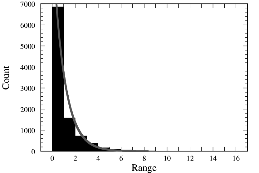
Figure 1: Theoretical distribution (gray line) superposed on frequency histogram for 10 000 event simulation of observations with $N=2$ Faraday excess rotation measurements.

The purpose of this demonstration is to show that the uncertainty in the mean-squared Faraday excess, for the best case obtained in the CKB survey, remains comparable with the result itself. It is manifestly clear that the uncertainty in this plot, i.e., its width, is commensurate with its mean value.

As a final illustration of the large measure of uncertainty, and motivated by the use by CKB of 16 Abell clusters, we consider the case $N=16$. The situation is similar to that encountered earlier, except that

$${\cal E}={\chi_{1}^{2}+...+\chi_{16}^{2}\over 16}\quad,$$ (21)

and that the joint probability distribution is the product of 16 Gaussians

$$p_{16}\left(\chi_{1},...,\chi_{16}\right)=\left\{{1\over\sqrt{2\pi\sigma^{2}}}\right\}^{16}\exp\left[-{\chi_{1}^{2}+...+\chi_{16}^{2}\over 2\sigma^{2}}\right]\quad.$$ (22)

Similarly, we observe that

$$\tilde{f}_{16}\left(k\right) = \left\langle\exp\left[ik{\chi_{1}^{2}+...+\chi_{16}^{2}\over 16}\right]\right\rangle$$ (23)

$$= \int_{-\infty}^{\infty}\cdots\int_{-\infty}^{\infty}\exp\left[ik{\chi_{1}^{2}+...+\chi_{16}^{2}\over 16}\right]\,\left[{1\over 2\pi\sigma^{2}}\right]^{8}\,\exp\left[-{\chi_{1}^{2}+...+\chi_{16}^{2}\over 2\sigma^{2}}\right]\,{\rm d}\chi_{1}\cdots{\rm d}\chi_{16}\quad.$$ (24)

The latter integral can be factored into 8 double integrals, each having the form seen in Eq. (14), thereby giving

$$\tilde{f}_{16}\left(k\right) = \left\{\int_{-\infty}^{\infty}\int_{-\infty}^{\infty}\exp\left[ik{\chi_{1}^{2}+\chi_{2}^{2}\over 16}\right]\,{1\over 2\pi\sigma^{2}}\exp\left[-{\chi_{1}^{2}+\chi_{2}^{2}\over 2\sigma^{2}}\right]\,{\rm d}\chi_{1}\,{\rm d}\chi_{2}\right\}^{8}$$ (26)

$$= {1\over\left(1-i{k\sigma^{2}\over 8}\right)^{8}}\quad,$$ (28)

where the role of $k$ has been replaced by $k/16$ and from which we obtain

$$f_{16}\left({\cal E}\right) = {1\over 2\pi}\int_{-\infty}^{\infty}\exp\left[-ik{\cal E}\right]\,\tilde{f}_{16}\left(k\right)\,{\rm d}k={1\over 2\pi}\int_{-\infty}^{\infty}{\exp\left[-ik{\cal E}\right]\over\left(1-i{k\sigma^{2}\over 8}\right)^{8}}\,{\rm d}k\quad{\rm for}\quad{\cal E}\geq 0$$ (29)

$$= \left({8\over\sigma^{2}}\right)^{8}{1\over 2\pi}\int_{-\infty}^{\infty}{\exp\left(-ik{\cal E}\right)\over\left(k+i{8\over\sigma^{8}}\right)^{2}}\,{\rm d}k={8\over 7!\,\sigma^{2}}\,\left({8\,{\cal E}\over\sigma^{2}}\right)^{7}\exp\left[-{8{\cal E}\over\sigma^{2}}\right]\quad.$$ (31)

The latter integral was evaluated by performing a contour integration in the lower-half plane and was evaluated using the calculus of residues at the compound pole at $-i8/\sigma^{2}$. It is easy to check that $\int_{0}^{\infty}f_{16}\left({\cal E}\right)\,{\cal E}=1$. We show in Fig. 2 this probability distribution function for the mean-squared FR excess (gray line) on a frequency histogram, once again superposing the result on a 10,000 sample Monte Carlo simulation. As pointed out before, the uncertainty in the mean-squared Faraday excess $\approx 35\%$ of the mean-squared estimate.

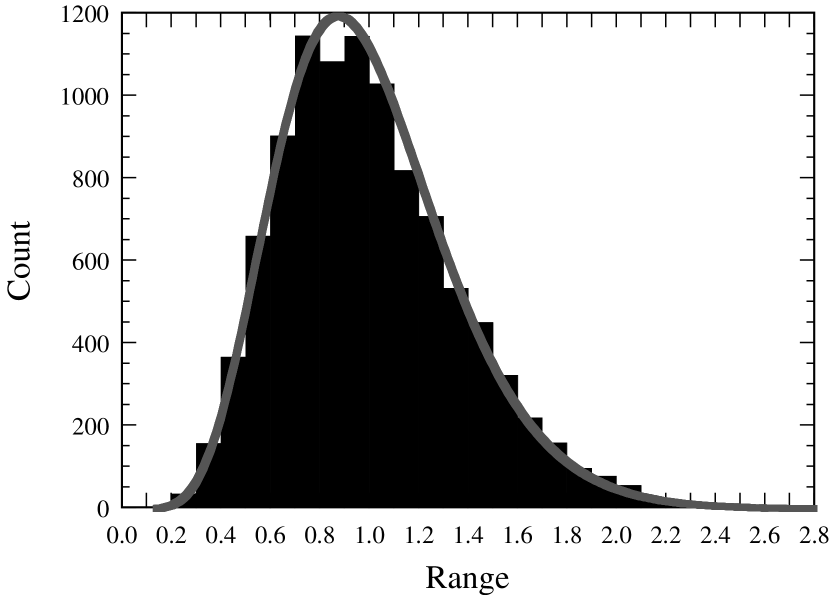
Figure 2: Theoretical distribution (gray line) superposed on frequency histogram for 10 000 event simulation of observations with $N=16$ Faraday excess rotation measurements.

We conclude that statistical limitations alone—without reference to any physical attributes involved in the measurement of FR—render the determination of magnetic fields by rotation measure-based techniques highly uncertain, with the uncertainty in the estimate being essentially the same size as the estimate itself. In effect, this result is the outcome of the “statistics of small numbers” (Newman et al.  1989), a not uncommon problem in astrophysics. Now, we wish to address some of the probabilistic or statistical issues that emerge from spatial heterogeneity in the fields.

3 Stochastic Field Coherence Effects

We explore here the role of spatial inhomogeneity in producing uncertainty in the estimation of IC magnetic fields. Earlier theoretical work by Crusius-Wätzel et al.  (1990) and Goldshmidt & Rephaeli (1993) considered the role of magnetic turbule size which they equated with the (reversal) coherence length, $\ell$, using straightforward random walk arguments. However, we will show, even if the mean value $\left\langle\ell\right\rangle$ is well-constrained in a given cluster, that its variability between clusters produces systematic effects that strongly influence our ability to estimate the magnetic field strength in the IC medium. The variation around the mean of some random quantities can systematically—i.e., in one direction—alter inferences of observed features, a point made by Newman et al.  (1995) in the context of radiative transfer. A related phenomenon is at work here, which we presently show.

In the paper by CKB, field strengths were inferred from their 16 Abell cluster survey assuming either a uniform slab geometry or random magnetic fields with fixed turbule size $\ell=10$ kpc, focusing especially on the latter case. To obtain further insight into this problem, we performed a Monte Carlo simulation corresponding to their observations. We assumed the magnetic field amplitudes—but not directions which were assumed to be random and isotropic—and that the thermal electron density ($n$) have a (commonly assumed) King profile,

$$n_{t}\left(r\right)={n_{0}\over\left(1+{r^{2}\over r_{c}^{2}}\right)^{{3\over 2}\beta}}\;,\;\quad r<R_{d}\quad.$$ (32)

Here, $r_{c}$ is the gas core radius whose value is in the range $1/4-1/3$ Mpc in nearby clusters; $\beta$ is an empirical coefficient with typical values between 1/2 and 3/4, and $R_{d}$ represents the outer limit to this density distribution, usually taken to be $\sim 10\ r_{c}$.

The unknown large scale profile of the locally averaged magnetic field is likely to be related to the gas density, particularly so if—as is likely—the fields were ejected from cluster galaxies together with metal-enriched gas. In this case the radial variation of the field strength can be assumed to vary as $n\left(r\right)^{q}$, with $q$ between 1/2 and 2/3, depending on whether magnetic energy or flux is conserved in this process (Rephaeli 1988). We can then write for the large scale variation of the field projected on the line-of-sight

$$B_{\parallel}\left(r\right)={B_{0}\over\left(1+{r^{2}\over r_{c}^{2}}\right)^{{3\over 2}\beta q}}\;,\;\quad r<R_{d}\quad.$$ (33)

where $B_{0}$ is the central value of the field. Also of interest is the limiting case of (essentially) identical field and gas profiles, $q=1$. Accordingly, we consider values of $q$ between 1/2 and 1. In our numerical estimates we use the central values $3\times 10^{-3}$ cm^-3, and 1 $\mu$G for the electron density and magnetic field, respectively. Finally, we assume that a characteristic value of $\ell$—the coherence length or magnetic turbule size—in a given cluster varies in the range $1-40$ kpc among the set of clusters, with a mean value of 10 kpc, corresponding to the selection made by CKB.

In order to suitably emulate the observations of CKB, we assumed that we were simulating observations of 16 Abell clusters with data derived from these, as shown in their tabulation of observational parameters. Just as the 27 observed data points were associated with their respective Abell clusters, we assumed that each of our simulated datum were associated with their respective and equivalently grouped hypothetical clusters. Further, we employed the “impact parameters” listed in Table 1 of CKB so that our numerical experiment could qualitatively behave in the same way as the observations. Our hypothetical clusters were parametrized using $r_{c}$, $R_{d}$, $\beta$, and $q$, as well as $\left\langle\ell\right\rangle$, which we fixed for each cluster. For each impact parameter $b$, we estimated $\chi$ by a numerical integration of Eq. (1), more precisely by using CKB’s formula (1), namely

$$RM=811.9\,\int_{0}^{L}n_{t}\,B_{\parallel}\,{\rm d}\ell\quad{\rm rad\ m^{-2}}\quad.$$ (34)

As a simple device for introducing the randomness associated with magnetic field orientations, we randomly selected the sign of the magnetic field computed from Eq. (22) along each line-of-sight segment of length $\ell$. Our simulation results are presented in Fig. 3 where RM values are shown against impact parameter for four hypotethical samples (each with 16 clusters). The distributions of physical parameters among these clusters are as follows: We assume that $r_{c}$ is uniformly distributed between 250 and 500 kpc, $R_{d}\equiv 10\,r_{c}$, $\beta$ is uniformly distributed between 1/2 and 3/4, and $q$ is uniformly distributed between 1/2 and 1. The four samples differ only in the assumed range of values of $\ell$. In order to allow as close a comparison as possible with the observational results of CKB, in our first sample we assumed $\ell=10$ kpc in all the clusters. Results of this simulation, shown in panel (a), closely mimic those of CKB, and this panel is qualitatively similar to their Figure (1) (open circles between 0 and 1500 kpc). Because of the very similar range of RM values in this panel and their figure, we use this panel as a ‘baseline’ case in the comparison of results shown in the other three panels.

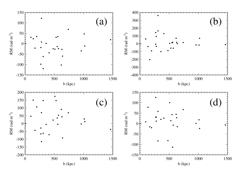
Figure 3: Rotation measure plotted as a function of source impact parameter for our four simulations. See text for details.

Before we do so we note that an absolute comparison between our results and those of CKB is somewhat uncertain since we use a realistic density profile and a range of values for the gas core radius. Nonetheless, we do not expect that these differences alone can account for the factor of $\sim 5$ larger field deduced by CKB from their observed range of RM values, the same range we have simulated with a central value of just 1 $\mu$G.

Taking $\ell$ to be uniformly distributed between 1 and 40 kpc yields the range of RM values shown in panel (b). Comparing panel (b) with panel (a), we see that the RM axis has expanded by nearly a factor of 3. What has happened here is that the simulated clusters having relatively large values of coherence length, i.e., $\ell>10$ kpc, contribute larger excess FR angles and this produces the greater scatter. Had this been an actual set of observations—and had we taken $\ell=10$ kpc—we would have inferred a value of $B_{0}$ that was a factor of 3 smaller than the fiducial field assumed in the simulation (1 $\mu$G). The contrast between these two panels makes it clear how sensitive inference can be to the assumed value of $\ell$.

We use two other distribution functions for $\ell$ in panels (c) and (d). In (c) we assume that $\ell$ is normally distributed with a mean of 20.5 kpc and a standard deviation of of 9.75 kpc, so that 2 standard deviations would span the range from 1 to 40 kpc. In (d) we use a log-normal distribution centered at $6.32$ kpc (the square root of 1 kpc $\times$ 40 kpc) with a variance (in the logarithm) of 2.51 (corresponding to the previous normally distributed case). The results shown in panels (c) and (d) again reveal the sensitivity to the distribution in $\ell$. In the normally distributed case, the generally higher values of $\ell$—compared with the “baseline” represented in panel (a)—result in generally larger values of RM. Again, if these were real observations, we would be obliged to infer a lower magnetic field, by nearly a factor of 2. However, in panel (d), the use of a log-normal distribution puts a heavy weight on generally lower values of $\ell$—the distribution was centered at 6.32 kpc. Had these been observations, we would have inferred a larger value for the magnetic field. At this stage in our investigation of the IC medium, it is not clear which (if any) of these panels is more representative of prevailing conditions. Accordingly, the likely physical variability of $\ell$ from one cluster to another makes an uncertainty in inferred fields of a factor of 2 highly probable.

As a final note in our discussion of the role of variability of coherence length and turbule sizes, we need also mention the likely variability of $\ell$ within a given cluster. Indeed, we are motivated by the expectation that the variability of the coherence length $\ell$ around its mean value $\left\langle\ell\right\rangle$ within a given cluster will be greater than the variability of the mean coherence length between clusters. Using simple random walk arguments, it is easy to show that the mean-squared Faraday excess satisfies

$$\left\langle\chi^{2}\right\rangle\propto\left\langle\ell^{2}\right\rangle$$ (35)

where the right hand side of the latter equation refers to the distribution of cell sizes. However, the Schwarz inequality applies in this situation; consider, therefore,

$$\left\langle\left(\ell-\left\langle\ell\right\rangle\right)^{2}\right\rangle=\left\langle\ell^{2}\right\rangle-{\left\langle\ell\right\rangle}^{2}\geq 0\quad,$$ (36)

with the equality satisfied only if $\ell$ is a constant, with no random variation. Thus, it follows that the use of a non-constant $\ell$ in our simulations of each of the clusters would have produced a systematically larger RM, thereby implying a smaller field when normalized to a given measured value of RM.

As a simple illustration of the significance of this result, suppose that the turbule sizes are Poisson distributed with mean $\ell_{0}$ in the IC medium, that is

$$p\left(\ell\right)={1\over\ell_{0}}\exp\left(-{\ell\over\ell_{0}}\right)\quad,$$ (37)

from which we obtain that

$$\left\langle\ell^{2}\right\rangle=2\ell_{0}^{2}{\rm\quad and\quad}\left\langle\ell\right\rangle=\ell_{0}\quad.$$ (38)

We note that a Poisson distribution of turbule sizes would introduce a factor of 2 into Eq. (24), that is, the right hand side should be a factor of 2 larger than would be obtained by assuming turbules of uniform size and that this would necessarily change the magnetic field estimate.

While the preceding illustration provides a hint as to the nature of the problem, deeper insight can be obtained by considering the possible dynamo origin of magnetic fields in galaxy clusters (Ruzmaikin et al.  1989, Zeldovich et al.  1988). Suppose that fully-developed, isotropic turbulence applies and that the distribution of turbule sizes can be related to a Kolmogoroff turbulent spectrum (Ferraro and Plumpton 1966). This could be the outcome of the injection of galactic fields into the IC medium, thereby “stirring” magnetized fluid contained within, resulting in the turbulent transport of energy from these largest scales to the smallest, dissipative scales. We will not consider in the present discussion the possibility that such turbulent activity could be further complicated by the emergence of rope-like structures, such as those mentioned by Ruzmaikin et al.  (1989) and Zeldovich et al.  (1988). The Kolmogoroff spectrum projected along a line-of-sight would have the characteristic $k^{-5/3}$ form, where $k=2\pi/\ell$ is the wavenumber that would characterize a turbule of size $\ell$. Accordingly, integrals containing terms like $k^{-5/3}\,dk$ would transform into $\ell^{-1/3}\,d\ell$ by virtue of $\ell=2\pi/k$. We now assume that the Kolmogoroff spectrum has lower and upper length-scale cut-offs, $\ell_{1}$ and $\ell_{2}$, respectively—these emerge from presence of dissipation and production ranges for the turbulence and we shall assume that $\ell_{2}\gg\ell_{1}>0$. In this environment, average values of any quantity $f\left(\ell\right)$ can be calculated according to

$$\left\langle f\left(\ell\right)\right\rangle={\int_{\ell_{1}}^{\ell_{2}}f\left(\ell\right)\,\ell^{-1/3}\,{\rm d}\ell\over\int_{\ell_{1}}^{\ell_{2}}\ell^{-1/3}\,{\rm d}\ell}\quad.$$ (39)

Hence, we find that

$$\left\langle\ell^{2}\right\rangle\approx{1\over 4}\ell_{2}^{2}{\rm\quad and\quad}\left\langle\ell\right\rangle\approx{2\over 5}\ell_{2}\quad,$$ (40)

and

$$\left\langle\ell^{2}\right\rangle={25\over 16}\left\langle\ell\right\rangle^{2}\quad.$$ (41)

We observe in this physically-relevant derivation that we recover a factor approaching 2 germane to our estimation of field strengths, and that the statistic emphasizes the longest turbule sizes (with a multiplying factor of 2/5). For the reasonable range of $1-40$ kpc, a representative mean turbule size would be $\sim 2/5\times 40=16$ kpc, rather than the fiducial 10 kpc that has (typically) been used.

The importance of this discussion regarding the variability of $\ell$ among clusters and inside each cluster is that this variability introduces further uncertainty, perhaps as much as an additional factor of 2, in our ability to estimate the prevailing magnetic fields. This magnetic turbulence-generated issue, together with the strictly statistical ones discussed in the previous section, introduce substantial uncertainties in values of the field deduced from FR measurements.

4 Radiative Compton-Synchrotron Measures of Magnetic Fields

Spectral and spatial measurements of the emission due to synchrotron and Compton energy losses of a population of relativistic   electrons can yield the electron spectral density distribution and magnetic field in the emitting region, and at least some information on the spatial profiles of these quantities. Over the large ($\sim 1$ Mpc) regions in clusters the electron density and magnetic field are expected to vary significantly, yet because of lack of adequate spatial information, this variation was ignored in all previous estimates of IC magnetic fields from radio and (NT) X-ray measurements (e.g.,  RGB, Fusco-Femiano et al.  1999). We now want to assess how such estimates are affected by the profiles of the relativistic   electrons and field.

Suppose that the electron Lorentz factor ($\gamma$) and radial ($r$) distributions are (separable and) given by

$$n(\gamma,r)=A\gamma^{-p}g(r),$$ (42)

and let the profile of the locally-averaged root mean squared field (over regions at least the size of $\ell$) be denoted by the function $b(r)$. The value of the field from radio and X-ray measurements is then proportional to the ratio (Rephaeli 1979):

$$\zeta=\left[{\int_{0}^{R_{d}}r^{2}g(r)dr\over\int_{0}^{R_{d}}r^{2}g(r)b(r)^{p+1\over 2}dr}\right]^{2\over p+1}$$ (43)

Likely deviation of the value of this ratio from unity introduced significant systematic uncertainty in the values of $B_{rx}$ that have previously been derived from radio and X-ray measurements.

To obtain some insight into how these geometrical considerations influence our estimates of $B_{rx}$, we have computed $\zeta$ for a variety of field and relativistic   electron profiles. Of these, perhaps most appropriate (since we have little information on the field and relativistic   electron spatial distributions) is to use the same functional form as that of the gas (eq. 21), but with a reasonably wide range of field and electron core radii, $r_{B},\,r_{e}$, respectively. The motivation for doing so is the expectation that field has likely originated in the cluster galaxies (Rephaeli 1988). Its spatial distribution is expected to be closely related to that of the hot gas, namely wide-spread throughout most of the cluster. The origin of relativistic   electrons is less clear; models range from origin in a few central radio galaxies (Rephaeli 1977), to ongoing shock acceleration by fast moving spiral galaxies (e.g.,  Bykov et al.  2001), implying a wider spatial distribution. (For more on electron models, see Sarazin 1999, and Rephaeli 2001.) Now, the observed regions of radio emission have sizes $\sim 1-2$ Mpc, and with $1/4-1/3$ Mpc as a typical range of gas core radii, it is clear that the field and electron profiles cannot be very centrally concentrated. On the other hand, it is also unlikely that either of these profiles—particularly that of the electrons—is more extended than that of the gas: Hot IC gas is a major, global component of clusters, whereas magnetic fields and relativistic   electrons are less ubiquitously abundant, and require special conditions to maintain, such as mechanisms for generation or amplification, and acceleration to balance energy losses, respectively.

In the table below we list some illustrative values of $\zeta$ computed for values of $r_{B}/r_{c}$ and $r_{e}/r_{c}$ in the range of $0.2-1$. While these results are general and do not depend on a specific value of $r_{c}$, we consider the lowest relevant values of $r_{B}$ and $r_{e}$ to be $\sim 50$ kpc, values corresponding to the lowest ratios in the table for $r_{c}=250$ kpc. We have taken the cluster limiting radius to be $10r_{c}$, and assumed that the sky-projected radius of the emitting region is $2r_{c}$, roughly corresponding to the region sampled by both the FR and radio measurements. The electron energy spectrum is assumed to be a power-law with index in the range $p=3-5$, i.e., corresponding to the range $1-2$ for the radio spectral index, $\alpha$. The best measured cluster radio spectrum is that of Coma, with $\alpha\simeq 1.34$ (Kim et al.  1991), implying $p\simeq 3.68$.

The factor $\zeta$ in the expression for $B_{rx}$

$r_{B}/r_{c}$	$r_{e}/r_{c}$		$\zeta$
		p=3.0	p=3.68	p=4.0	p=5.0
0.2	1.0	24.0	17.9	15.8	11.4
	0.6	20.7	15.7	14.0	10.3
	0.2	13.5	10.9	9.9	7.7
0.6	1.0	5.2	4.7	4.5	3.9
	0.6	4.6	4.2	4.0	3.6
	0.2	3.4	3.2	3.1	2.8
1.0	1.0	2.9	2.7	2.7	2.5
	0.6	2.6	2.5	2.5	2.3
	0.2	2.1	2.0	2.0	1.9

We see that $\zeta$ (which is always $>1$) assumes values in the interval $\simeq 2-24$ for the range of core radii taken here. Specifically, in the Coma cluster—using the measured radio and (assumed Compton) X-ray fluxes, and ignoring the unknown spatial profiles (effectively, taking $\zeta=1$), RGB deduced a value of $\sim 0.2$ $\rm\mu G$ for $B_{rx}$, which we denote here as $B^{U}_{rx}$. This fiducial value is to be contrasted with the estimates based on $\zeta\neq 1$: Had RGB assumed the above field and electron profiles and parameters, they would have deduced values of $B_{rx}$ in the center of the cluster which are in the range $\sim 0.4-4.8$ $\rm\mu G$.

Having illustrated the impact of spatial profiles of the gas, field and electrons, we should emphasize that even though these profiles are realistic, the viable ranges of core radii are likely to be narrower than considered here. The latter will only be known once detailed measurements are made of the spatial distributions of the radio and NT X-ray emission. It is also important to note that the volume-averaged mean field value is generally lower than the product $B^{U}_{rx}\times\zeta$ by a factor that depends very much on the way this average is defined.

5 Discussion

We have explored several sources of uncertainty in the estimation of magnetic field strengths in clusters. The first of these, related to the measurement of excess FR, is of a purely statistical source and, in essence, is the outcome of the statistics of small numbers. The lack of large numbers of clusters that can be adequately probed by this technique results in an uncertainty in the estimate of the mean-squared excess FR that is comparable with the estimate itself. The second of these has a more physical basis, yet is due to the underlying randomness in the spatial structure of turbulent magnetic fields. The variability of the coherence length or magnetic turbule size within each cluster and among clusters can introduce uncertainties in the field approaching an order of magnitude. Finally, the traditional use of Compton and synchrotron emissions to determine IC field strengths requires knowledge of the unknown field and relativistic   electron morphologies, introducing yet another source of uncertainty, one that could easily translate to a factor of at least a few in the value of the deduced mean field.

A realistic assessment of the above uncertainties is of obvious relevance to the study of nonthermal phenomena in general, and to the modeling of the origin of the fields and energetic electron populations in particular. Mean field values of ${\cal O}(10^{-7})$ G can be comfortably expected from ejected galactic fields, but not so if the mean field value is ${\cal O}(10^{-6})$ G. The implied electron energy density, $\rho_{e}\propto B^{-(p+1)/2}$, depends steeply on B. An uncertainty of a factor of a few in B typically implies more than an order of magnitude difference in $\rho_{e}$ (and the related energetic proton energy density). This too can make all the difference in judging the viability of models for particle origin and the need for effective re-acceleration processes in the IC space.

Of course, the range of electron energies implied from the observed radio spectral range also depends directly on the field value, though much less steeply ($\gamma\propto B^{-1/2}$), than the energy density. The lower the field value, the higher is the energy of the synchrotron emitting electron, and the shorter is its (dominant radiative) Compton energy loss time ($\propto 1/\gamma$). A short loss time could mean either that radio and X-ray emission might be short, essentially transient phenomenon, or that the particles are continually accelerated in order to sustain these emissions over cosmological time.

As mentioned in the Introduction, the electron energy spectrum is likely to extend to energies well below the range probed directly by radio measurements. Indeed, in the simplest model, if a steady state is attained then relativistic   electrons are continually replenished as they lose energy, first radiatively and then by electronic (Coulomb) excitations (e.g., , Rephaeli 1979). For any reasonable mean IC magnetic field value, only high energy ($\gamma>10^{3}$) electrons contribute to the observed radio emission. Therefore, if the electron energy spectrum is correctly extended to lower energies (by taking Coulomb losses into account) then this will not have appreciable impact on our above considerations. If, on the other hand, an energetic electron population is conjectured in order to account for the claimed measurement of EUV emission in the Coma cluster, then extension of this population to higher energies may in general imply a higher magnetic field (e.g., , Sarazin & Kempner 2000) then our deduced values of $B_{rx}$. However, the proposed energetic electron models are quite unrealistic due to their very high energy densities, which are comparable to or even higher than the gas thermal energy density (Rephaeli 2001, Petrosian 2001).

The CKB core sample consisted of 27 radio sources, only 12 of which were background sources. The inclusion in the sample of a large fraction of cluster members introduces an additional uncertainty which stems from the possibility that these sources have (statistically) different radio properties from those of the background sources, and the expectation that the IC pathlength for a cluster member is on average only half that of a background source. The issue whether the mixed nature of such a sample affects estimates of the mean IC field was previously investigated by Goldshmidt & Rephaeli (1993) in their re-analysis of the Kim et al.  (1991) sample. By repeating the analysis of FR measurements of cluster vs. non-cluster members, Goldshmidt & Rephaeli (1993) concluded that the distribution of rotation angles of cluster members was actually somewhat narrower than that of non-cluster members, perhaps due to the reduced pathlength of the former sources. This difference was small enough that estimates of the field were hardly affected. The issue has to be further explored before definitive statements can be on the magnitude of the systematic uncertainty due to a ‘mixed’ radio sample.

The systematic uncertainties we have expanded upon should be better understood and more explicitly acknowledged whenever values of the field (and electron energy density) are reported. This is crucial when values of $B_{fr}$ and $B_{rx}$ are compared. In particular, we caution against strong conclusions that are sometimes drawn on the non-viability of the Compton interpretation of NT X-ray emission based on the discrepancy between deduced values of $B_{fr}$ and $B_{rx}$. As we have clearly demonstrated here, the current status of the measurements, and their associated substantial uncertainties, render such conclusions premature.

References

- Bowyer et al. (1998) Bowyer, S., & Berghofer, T.W. 1998, ApJ, 506, 502
- Bowyer et al. (1999) Bowyer, S., Berghofer, T.W., & Korpela, E.J. 1999, ApJ, 526, 592
- Bykov et al. (2000) Bykov, A. et al. 2000, A&A, 362, p.29
- Clarke, Kronebrg and Böhringer (2001) Clarke, T.E., Kronberg, P.P., & Böhringer, H. 2001, ApJ, 547, L111