The Starlab Environment for Dense Stellar Systems

Abstract

Traditionally, a simulation of a dense stellar system required choosing an initial model, running an integrator, and analyzing the output. Almost all of the effort went into writing a clever integrator that could handle binaries, triples and encounters between various multiple systems efficiently. Recently, the scope and complexity of these simulations has increased dramatically, for three reasons: 1) the sheer size of the data sets, measured in Terabytes, make traditional ‘awking and grepping’ of a single output file impractical; 2) the addition of stellar evolution data brings qualitatively new challenges to the data reduction; 3) increased realism of the simulations invites realistic forms of ‘SOS’: Simulations of Observations of Simulations, to be compared directly with observations. We are now witnessing a shift toward the construction of archives as well as tailored forms of visualization including the use of virtual reality simulators and planetarium domes, and a coupling of both with budding efforts in constructing virtual observatories. This review describes these new trends, presenting Starlab as the first example of a full software environment for realistic large-scale simulations of dense stellar systems.

Institute for Advanced Study, Princeton, NJ 08540, U.S.A.

1. A Brief History of Simulations of Dense Stellar Systems

Modeling a star cluster on a computer is a subject with a published history of more than forty years, starting with the 10-body simulations by von Hoerner (1960). These pioneering calculations had to be halted when the first binary was formed. In those days neither was the hardware fast enough, nor the software sophisticated enough to follow the long-term evolution of a perturbed binary. Rapid improvement of both hardware and software allowed the treatment of dynamically formed binaries by the mid-sixties, but the maximum number of bodies remained in the regime $N<100$ where relaxation effects could not be ignored on a crossing time. By the early seventies, larger systems could be modeled, up to $N=500$. By that time a clear separation between relaxation time and crossing time could be observed.

These simulations showed that the core of a typical star cluster contracts as a result of heat flowing toward its outer regions, on a two-body relaxation time scale. This phenomenon had been predicted theoretically and was dubbed ‘gravothermal collapse’ or ‘core collapse’, where the term ‘collapse’ is perhaps a bit misleading since the process takes billions of years for a typical globular cluster. It was observed in the simulations that this type of collapse continues until a hard binary appears in the center, where the term ‘hard’ indicates that the binary has a binding energy much larger than the typical kinetic energy of a single star. Such binaries tend to give off energy to passing stars, hardening even further while heating their surroundings. In this way, one or more hard binaries were observed to provide the heat source that balanced the heat losses further out in the star cluster, thus ending core contraction. Just as an individual star like the sun balances radiation losses from its photosphere with nuclear energy generation in its core, after the initial contraction of the protostar toward the main sequence, star clusters with a ‘collapsed core’ can similarly balance their energy budget.

Key ingredients in making it possible to integrate these larger 500-body systems in the seventies were the use of individual time steps (Aarseth 1963), as well as special treatments of binaries through various ways of analytical and other forms of regularization (cf. Aarseth 1985, 2002). By the late eighties the mechanism of core collapse had been fully understood, including the conditions for the occurrence of post-collapse core oscillations, using numerical simulations in the conducting gas sphere approximation (Sugimoto & Bettwieser 1983, Bettwieser & Sugimoto 1984), Fokker-Planck approximation (Cohn et al. 1989, Murphy et al. 1990) as well as semi-analytical arguments (Goodman 1987). The first demonstration of the occurrence of core oscillations in direct $N$-body systems was given by Makino (1996), using the GRAPE-4 to perform a 32,000-body calculation, a tour de force around that time. Only now, six years later, are simulations of this size becoming more routine. For a review of the GRAPE project, see Makino (2002) and Makino & Taiji (1998).

From an astrophysics point of view, $N$-body simulations of star clusters have finally started to become realistic, over the last few years, now that stellar evolution recipes have been tightly coupled to stellar dynamical calculations. The talks at this symposium by Hurley (2002) and McMillan (2002) give pointers to the literature. For more general background information, see Heggie & Hut (2002). Most interesting and most challenging are the treatments of multiple stellar encounters: interactions between binaries and single stars, binary-binary encounters, or even more complex interactions involving, say, an encounter of a triple and a binary, or an encounter of a binary with an interacting tangle of stars in which other multiples have already temporarily been captured. Following such complex interactions poses severe challenges to the development of software needed to choreograph these many-body dances. Let us look at one such system, Starlab, the most advanced in design for simulating dense stellar systems.

2. A Software Environment: Starlab

Starlab is a software package for simulating the evolution of dense stellar systems and analyzing the resultant data. It is a collection of loosely coupled programs (‘tools’) linked at the level of the UNIX operating system. The tools share a common data structure and can be combined in arbitrarily complex ways to study the dynamics of star clusters and galactic nuclei. Although most tools are written in C++, Fortran programs and subroutines can be easily included, as well as programs written in other languages. The package is publicly available through our web site $<$http://www.manybody.org$>$, where links can be found to Starlab, as well as to other packages, such as the Nemo environment (for collisionless stellar dynamics). For a description of the main Starlab components, see Portegies Zwart et al. (2001).

Starlab features the following basic modules:

• Three- and four-body automated scattering packages, constructed around a time-symmetrized Hermite integration scheme.

• A collection of initialization and analysis routines for use with general N-body systems.

• A general Kepler package for manipulation of two-body orbits.

• N-body integrators incorporating both 2nd-order leapfrog and 4th-order Hermite integration algorithms.

• Kira, a general N-body integrator that automatically applies local coordinate transformations in a recursive way, allowing uniform treatment of hierarchical systems of arbitrary complexity within a general N-body framework.

• SeBa, a stellar evolution and binary evolution package that follows the evolution of any star or binary from arbitrary initial conditions, or from later starting conditions following a dynamical interaction.

A novel aspect of Starlab is its flexible external data representation, which guarantees that tools can be combined in arbitrary ways, without loss of data or internally-generated comments. Thus, two tools connected by UNIX pipes may operate on different portions of the same data set, even though neither understands the data structures, or even the physical variables, used by the other. Unknown data are simply passed through unchanged to the next tool in the chain.

This feature is especially important for simulations that include the use of both Kira and SeBa. Although the two programs are linked at compile time, before being run, we have gone to great length to guarantee maximal decoupling between the structures of the two programs. Conceptually we have the following picture:

where the data passing currently takes place via an exchange through a well-defined and minimal interface between the C++ objects that represent the dynamical part of a star and the stellar evolution aspects of that same star.

We are currently planning the next great leap forwards, which will entail three significant improvements. The first is to replace stellar evolution recipes by actual stellar evolution codes. The second is to replace code linking by the more flexible mechanism of message passing. The third is to introduce some form of stellar hydrodynamics code, to model the details of stellar collisions. Conceptually, our goal is to model a dense stellar system as follows:

Let us look at each of these three aspects – stellar evolution, hydrodynamics, and code communication – in turn.

3. Truly Interacting Stars

It is a well kept secret that stellar evolution codes cannot follow the full lifetime evolution of a star from beginning to end without human intervention. Modeling the main sequence evolution presents no difficulties, but rapid changes occurring in later stages of stellar evolution will either lead to a crash of the code or to such a slow crawl that the run cannot be completed in a reasonable time. This does not pose a serious problem when we want to make a detailed study of a particular star. In that case we may not be interested in the most unstable phases of its evolution; or if we are, we can help the code along by some suitable choice of parameter changes when necessary.

This state of affairs does pose a serious problem, however, when we want to use a stellar evolution code as a module in a larger system of a hundred thousand stars or more. In that case it would be totally impractical to tweak the late stages of evolution of individual stars by hand. The obvious solution is to simplify stellar evolution codes, letting them skip over some of the most numerically sensitive episodes in their evolution. While this introduces errors, it is surely better than having no information at all about the late-time behavior of the stars. And as long as we can keep track of the approximations involved, we can try to decrease the errors in due time, when faster future computers allow us to spend more CPU time on an individual star.

If we only had to deal with single stars, one could argue that it would be better to use the best codes available, together with a very patient lab assistant who coaxes the code through the difficult stages in its evolution, time and again, for a wide choice of parameters, such as initial mass and initial chemical composition. After producing a multidimensional collection of stellar evolution tracks, the values can be stored in tables, or complicated parameter fits can be made. For each star in a star cluster simulation, the physical parameters describing the stellar structure and composition of a star can then be obtained automatically from the tables or fits.

While this may well be the best approach for dealing with single stars, it will not work for interacting double stars. As soon as one of the stars transfers mass to the other star, the evolution of both stars will begin to diverge from the standard tracks obtained for single stars. What will happen next depends on several parameters: the mass of each of the stars, the initial separation between the stars, the chemical composition of each of the stars. Even if we assume both stars to have the same composition labeled only by metallicity, we suddenly find ourselves with a four-parameter family of pairs of evolution tracks that will need to be tabulated or fitted, in addition to those of the single stars.

And as if that would not be sufficiently impractical, we also have to deal with blue stragglers, stars that have been formed through a merger of two or sometimes even more than two stars. And then there are triple stars, where the outer star can perturb the orbit of the inner two stars, thereby modifying the rate of mass transfer considerably. It is clear that the use of canned stellar evolution tracks is not going to help us here. There seems to be no other choice than to enlist the help of a real stellar evolution code, albeit a simplified one. Such a stellar evolution module should be able to produce results that are at least somewhat reasonable without any need for human hand-holding, and in a rather short amount of computer time.

For example, when we follow $3\times 10^{5}$ stars, of which 10% are part of a primordial binary, there is a potential need to model $3\times 10^{4}$ stars separately. However, many of those binaries will be wide enough to avoid contact, while others may merge quickly and therefore do need much CPU time. As a round estimate, perhaps 1% of the stars will need to be followed in great detail, during the simulation of the full history of the star cluster. If we have one or more fast front end computers connected to a cluster of GRAPE-6 boards, the total star cluster simulation might be completed in a few months. Dividing this total CPU time of $10^{7}$ seconds over the $3\times 10^{3}$ problem stars, we are left with up to an hour per star (even more if we have several CPUs working together on the simulation). This is more than enough for a simple modeling job, and it is clear that CPU time is not the bottle neck. The only real problem lies in the software: there is an urgent need for simple but robust stellar evolution codes.

It may even be feasible to model all stars, single or double, by direct calculation. This would take away the need for the additional complexity in the form of tables and fitting functions. Depending on the number of CPUs in the front end, such a brute-force approach would leave us with a minute or several minutes per star. For single stars, this may already suffice; and if not now, then in the near future, with the next generation of faster computers.

4. Hydrodynamics

When two stars in a binary exchange mass in a stable way, on a thermal time scale (with the donor star typically the less massive of the two), it is relatively straightforward to couple two stellar evolution programs together. At the moment of first contact, we already know the precise structure of each star, and if we continue to use a simple spherical approximation for the shape of each star, we only have to change the boundary conditions. Mass shed from the donor star will be taken from its outer layers, and added to the outer layers of the receiving star. Dynamical equilibrium can be easily enforced right away, and the two stars will then take care of the restoration of thermal equilibrium automatically, in the course of their subsequent evolution.

Things get quite a bit more complex when two stars collide. This can occur during an unstable phase of mass transfer, for example when the heaviest star transfers matter to the lighter star. Conservation of angular momentum then tends to decrease the distance between the stars, leading in most cases to further mass transfer, resulting in a spiral-in of the two star cores in their common envelope. Other scenarios leading to stellar collisions include random encounters between single stars in the dense cores of stellar systems, as well as local encounters within interacting systems of three or more stars.

The simplest example of the latter occurs when a binary and a single star meet each other. While there is already a chance for a collision between two or perhaps all three stars during the initial encounter, the collision probability is significantly enhanced when the three stars are temporarily captured in what is called a resonance scattering event (cf. Heggie & Hut 2002). If the stars would truly be point masses, such an unstable three-body system would ultimately fall apart again into a single star and a double star, but the stars may conduct tens or hundreds of passes through the system before finally escaping. Even in relatively wide configurations, the cumulative chance for collisions between at least two of the stars during this protracted dance can be considerable.

In most star clusters a significant fraction of the stars are born in binaries. The probability for two of these primordial binaries to meet each other is relatively high, given the fact that binaries tend to sink to the core of a star cluster on a two-body relaxation time scale, as a result of mass segregation. When four stars meet each other to form a temporarily bound subsystem, the chance for collisions is even higher than in the three-body case, given that there are six pair-wise permutations for which collisions can take place.

The first case mentioned, that of common-envelope evolution, is the hardest one to model. We are dealing with a three-dimensional problem in hydrodynamics, where the initial stages of slow spiral-in can cover a very large number of orbital periods. In contrast, collisions in the other scenarios are almost instantaneous events. The effects of a collision between two stars make themselves felt within the interiors of the stars on a sound crossing time, of order an hour for a main sequence star. Even if a single star passes through a red giant, the collision between the star and the core of the giant will take place on a time scale of hours; and if the star misses the core, the chance is high that no merger will take place at all.

Collisions can be modeled with modest accuracy by using a simple hydrodynamics code, preferably an SPH code. Here SPH stands for Smooth Particle Hydrodynamics, where each particle carries not only a mass, position and velocity, as in stellar dynamics, but also an entropy. With each particle thus representing a fluid element, it is easy to model systems with extreme density contrasts, especially if different particles are allowed to have different masses. With a dynamic particle splitting and merging scheme, it then becomes possible to model both the low-density exteriors as well as the high-density cores of stars involved in a collision.

The central idea is to represent each star by a single mass point together with a stellar evolution module (either a canned stellar evolution track or an simple real-time stellar evolution code), during most of the lifetime of a star. Only just before a strong encounter will the single mass point be replaced by a whole cloud of SPH particles. The internal structure of the SPH object, such as density, temperature and chemical composition as a function of radius, can be determined from the information carried in the stellar evolution module. After the strong encounter is finished, the SPH objects should be given some extra time to settle down on a dynamical time scale. Finally, each object can be collapsed back into a point, to take part once again in the overall dynamical $N$-body dance of the star cluster as a whole.

A major complication in this last stage of transformation is the question of how to update the stellar evolution module of each SPH object. The radial distribution of temperature, density and chemical composition can be read off with limited accuracy from the cloud of SPH particles. The challenge is then to construct a new stellar structure model for the object, as a new starting model for the subsequent stellar evolution calculations. Since the stellar structure at this point is likely to be far off from thermal equilibrium, there may not be any standard model available to use as a guiding tool. Again, we must insist on the stellar evolution code to be smart enough to find a new starting model anyway, without any human guidance.

5. Message Passing

Our first goal is to have primitive working versions in place of an hydrodynamics code and a stellar evolution code, together with an implementation of the rather complex administrative rules that guide their interaction with each other and with the leading stellar dynamics code. While this already poses quite a few challenges, it is only part of what is required for a full simulation of a star cluster. To make everything work, we have to find ways to couple everything together.

Traditionally, this is done by linking the various modules together at compile time. Each module then acts pretty much as a subroutine in a Fortran program. And while each module can be compiled and tested separately, in the end they together form one massive program where in principle everything is coupled. For an intermediate-size software project, this may not be such a bad thing. A good programming style can go a long way to ensure some form of data abstraction and separation. For example, avoiding the use of global variables (or common blocks when programming in Fortran) would be a good start.

However, the larger the total program becomes, the greater are the dangers of unintended interactions between its parts. This will make debugging increasingly difficult. Since different people will write and maintain different modules, debugging will probably require interactive collaboration between those individuals, further complicating overall code maintenance. Clearly, by the time we have complex working codes for stellar dynamics, stellar evolution, and stellar hydrodynamics, we have to look for better ways to integrate everything.

In theoretical astrophysics, so far there has been little need to go beyond the model of working with a handful of program files, linked together at compile time. But in various areas of software development, starting a couple decades ago, other solutions have been explored in order to deal with increasingly complex configurations of interacting programs. An example is the X window system developed at M.I.T. in the early to mid eighties. Since X is open source, it has been extended widely every since; see $<$http://www.X.org/about_x.htm$>$ for a brief introduction. The core ideas in X are to run the different modules asynchronously, without a single core program telling each module what to do and when.

This lack of centralized control allows much greater freedom for the construction and maintenance of individual modules. Each module can be regarded as a black box with a well-defined protocol that allows for exchange of information between the boxes. Communication takes place through message passing, in a client-server model. One module can send a message to another module, which then leads to the appropriate action as soon as possible given the other demands on that module. As with any form of parallelism, an appropriate tuning of priority levels (hopefully) leads to a reasonable minimization of overall waiting times, depending on the ramifications of each request.

We are currently contemplating a somewhat similar implementation for a master framework that will allow stellar dynamics, evolution, and hydro codes to talk to each other. Such a framework, once in place, will make it trivial to mix and match modules written in different styles and in different computer languages. All that is needed for a new module to be installed, or for a current module to be replaced, is to agree upon the interface protocol, including the set of data that can be exchanged and their precise formatting. We hope to start this development, from X windows to ‘windows on the Universe’ in the near future.

6. An Extended Software Environment

Currently, Starlab does not have a fully working hydrodynamics module, although we have experimented with some toy models as a proof of concept for translating $N$-body particles into polytropic star models realized in SPH, and vice versa. Also, Starlab has not yet incorporated real stellar evolution codes. So far, all effects related to stellar structure and evolution have been handled by the SeBa package mentioned in section 2, which relies on formulas fitted to previously computed stellar evolution tracks (such as given by Hurley et al. 2000).

Even with those restrictions still in place, we have recently encountered the need for additional software improvements, mainly as a result of a vast increase in data throughput. The source of this good news is the fact that a large number of GRAPE-6 boards have come on-line, in the form of the 48-Teraflops cluster in Tokyo as well as smaller clusters elsewhere in the world. This has made it possible for us to model small globular clusters on a star-by-star basis for the duration of a Hubble time. However, the Terabytes of data produced by those runs have posed new challenges in the areas of flexible visualization, efficient archiving, and the exchange of data with other groups. Let us briefly discuss each of these three challenges (see figure 1 for an overview).

6.1. Visualization

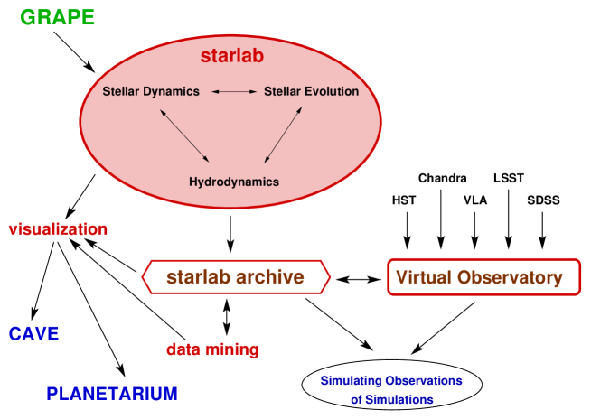
Figure 1.: A software environment for simulations of dense stellar systems. Centered around Starlab, it contains connections with a library of GRAPE routines, with various visualization tools, and with an archive to store the most interesting runs. In addition, it will maintain links to virtual observatory initiatives.

We have started to explore the possibility of using planetarium domes to create a fully immersive interactive virtual reality environment to display the 4-D space-time data from a complete globular cluster simulation history. Using software developed at NCSA for their CAVE (cf. $<$http://evlweb.eecs.uic.edu/pape/CAVE$>$), and later adapted to the dome in the Hayden Planetarium at the American Museum of Natural History, we have been able to ‘fly through’ our star clusters in space and time. In contrast to a computer screen, which forces the user to zoom in and out repeatedly in order to get a complete picture of what is going on, a dome allows the user to retain the global view while at the same time focusing on individual interaction regions. The extra resolution afforded by a set of seven projectors (two covering the ‘polar cap’, and five covering the azimuthal sweep along the ‘horizon’) makes this simultaneous local-global investigation possible. See Teuben (2002) and Teuben et al. (2001, 2002) for more details.

6.2. Archives

With the ability to visualize the complete history of a small globular cluster on a star-by-star and orbit-by-orbit basis, it would be a shame not to store the appropriate data set from, say, a month-long run on a GRAPE-6 cluster. Fortunately, not every position and velocity value has to be stored for each star at each time step. Experimentation has shown that storing only a few percent of those data suffices to reconstruct the orbits through higher-order interpolation, to a degree that is virtually indiscernible from the real thing, to the human eye. Even so, this leaves us with the need to archive Terabytes of data for our largest runs, in such a form that it will be relatively easy to extract information sliced in space as well as in time. In some cases, we may want to display snapshots of the whole system. In other cases, we may be interested on what happened to only a handful of interacting stars, but over a much longer period of time. We are currently experimenting with different ways to solve these conflicting demands efficiently.

6.3. Virtual Observatories

The challenge of dealing with enormous data sets has hit observational astronomy long before it has become a problem for theoretical simulations. In various countries new initiatives have started to address these problems through the construction of what are called virtual observatories. These will provide portals on the internet that allow the user to become a virtual observer, ‘observing’ data available in archives from major observatories, ground-based as well as space-based. In addition, the user will be able to correlate information from and submit queries to a diverse range of sources. All this is still in its initial stages, but the results so far are already promising. See the proceedings of the recent conference Virtual Observatories of the Future (Brunneret al. 2001), or the NVO website $<$http://nvosdt.org$>$ for pointers to the U.S. initiative as well as to parallel efforts in other countries.

7. Summary

We are now at the verge of simulating the full history of a globular cluster on a star-by-star basis, following each star dynamically while also modeling their stellar evolution. Initially we will use 100,000 stars, and we hope to extend this number to 300,000 or more; by the end of the decade, with Petaflops computers such as the GRAPE-8, we may reach our holy grail of accurately modeling a million stars for 10 billion years, while resolving local interactions involving binaries and more complex systems on time scales of hours and days.

We expect to deliver two rather different types of results, one oriented to observations, one to theory. On the observational side, we would like to give visitors the option to look at our simulated clusters at any time and distance of their choice, through whatever instrument they like (say, in a given wave length band, using the Hubble Space Telescope, at a distance of 5 kpc when the cluster was 8 billion years old; or using Chandra, the VLA, etc.).

On the theoretical side, we can use our largest runs to provide access to other theorists who have more specific questions about particular objects. For example, if we are interested in finding out how binary pulsars are formed, through what channels and with what type of eccentricity distributions, we have no choice but to run a full simulation of a star cluster, and then to pick out the binary pulsar related events. However, this same simulation will allow others to analyse in detail what happened with the CVs in the system, the blue stragglers, as well as many other variable stars and binaries, triples, etc. So we will invite not only ‘guest observers’, but also ‘guest theorists’ who can pick their favorite objects from our simulation and compare our space-time trajectories and interactions of those objects with their own analytical and/or numerical attempts to model them in isolation. Their modeling may be more detailed but we provide a more realistic context, thus providing complementary ways to shed light on the objects of interest.

We currently have three essential ingredients in place to do these jobs: access to a super-fast computer, the GRAPE-6 running at 48 Teraflops in Tokyo; the software to run our simulations in the form of the Starlab environment; and an opportunity to visualize our results using the Hayden Planetarium dome at the American Museum of Natural History in New York City. What is needed now is further software development, both within and around Starlab. Within Starlab we plan to introduce stellar evolution codes as well as hydrodynamics (SPH) codes, together with a message passing framework to connect both type of codes with each other and with the Kira code that governs the stellar dynamics. Around Starlab we plan to improve our use of partiview, the open source version of the Virtual Director software used in the Hayden dome; to create Starlab archives; to develop software for guest observers; and to establish links to virtual observatories.

I acknowledge support from the Alfred P. Sloan foundation, through a grant for research at the Hayden Planetarium of the American Museum of Natural History in New York.

References

- 1963 Aarseth, S. J. 1963, MNRAS126 223
- 1985 Aarseth, S. J. 1985, in Multiple Time Scales, ed. J.U. Brackbill and B.I. Cohen (New York: Academic), p. 377
- 2002 Aarseth, S. J. 2002, these proceedings.
- 1984 Bettwieser, E. and Sugimoto, D. 1984, MNRAS 208, 439
- 1989 Brunner, R.J., Djorgovski, S.G., and Szalay, A.S. (eds.), 2001, Virtual Observatories of the Future, ASP Conference Series, Vol. 225 (San Francisco: ASP).
- 1989 Cohn, H., Hut, P. & Wise, M. 1989, ApJ 342, 814
- 1987 Goodman J. 1997, ApJ313, 576
- 2002 Heggie D.C. and Hut P. 2002, The Gravitational Million-Body Problem [Cambridge University Press]
- 2002 Hurley, J.R. 2002, these proceedings.
- 2000 Hurley, J.R., Pols, O.R. and Tout, C.A. 2000, MNRAS 315, 543
- 1996 Makino J. 1996, ApJ471, 796
- 1998 Makino J. and Taiji M. 1998, Scientific Simulations with Special-Purpose Computers — The GRAPE Systems, John Wiley and Sons, Chichester.
- 2002 Makino, J. 2002, these proceedings.
- 2002 McMillan, S. 2002, these proceedings.
- 1990 Murphy, B.W., Cohn, H.N. & Hut, P. 1990, MNRAS, 245, 335
- 2001 Portegies Zwart, S.F., McMillan, S.L.W., Hut, P. and Makino, J. 2001, MNRAS321, 199.
- 1983 Sugimoto, D. and Bettwieser, E. 1983, MNRAS 204, 19p
- 2002 Teuben, P.J. 2002, these proceedings.
- 2001 Teuben, P.J., Hut, P., Levy, S., Makino, J., McMillan, S., Portegies Zwart, S., Shara, M., and Emmart, C. 2001, in Astronomical Data Analysis Software and Systems X, eds. Harnden, Jr. F.R., Primini, F.A. and Payne, H.E., ASP Conference Series, Vol. 238 (San Francisco: ASP), 499.
- 2002 Teuben, P.J., De Young, D., Hut, P., Levy, S., Makino, J., McMillan, S., Portegies Zwart, S., and Slavin, S. 2002, in Astronomical Data Analysis Software and Systems XI, ASP Conference Series (San Francisco: ASP), to appear.
- 1960 von Hoerner, S. 1960, Zeitschrift fuer Astrophysik, 50, 184