The discovery of X–rays from Venus with Chandra

Abstract

On January 10 and 13, 2001, Venus was observed for the first time with an X–ray astronomy satellite. The observation, performed with the ACIS–I and LETG / ACIS–S instruments on Chandra, yielded data of high spatial, spectral, and temporal resolution. Venus is clearly detected as a half–lit crescent, with considerable brightening on the sunward limb. The morphology agrees well with that expected from fluorescent scattering of solar X–rays in the planetary atmosphere. The radiation is observed at discrete energies, mainly at the O–K_α energy of 0.53 keV. Fluorescence radiation is also detected from C–K_α at 0.28 keV and, marginally, from N–K_α at 0.40 keV. An additional emission line is indicated at 0.29 keV, which might be the signature of the C $1s\to\pi^{\star}$ transition in CO₂ and CO. Evidence for temporal variability of the X–ray flux was found at the $2.6\,\sigma$ level, with fluctuations by factors of a few times indicated on time scales of minutes. All these findings are fully consistent with fluorescent scattering of solar X–rays. No other source of X–ray emission was detected, in particular none from charge exchange interactions between highly charged heavy solar wind ions and atmospheric neutrals, the dominant process for the X–ray emission of comets. This is in agreement with the sensitivity of the observation.

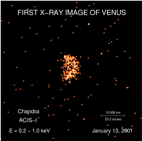
Figure 1: Chandra ACIS–I image of Venus.

1 Introduction

In January 2001 we observed Venus for the first time ever with an X–ray telescope (Fig. 1, Tab. 1). Orbiting the Sun at heliocentric distances of 0.718 – 0.728 astronomical units (AU), the angular separation of Venus from the Sun, as seen from Earth, never exceeds 47.8 degrees (Fig. 2). While the observing window of imaging X–ray astronomy satellites is usually restricted to solar elongations of at least $60\degr$, Chandra is the first such satellite which is able to observe as close as $45\degr$ from the limb of the Sun. Thus, with Chandra an observation of Venus with an imaging X–ray astronomy satellite became possible for the first time. The observation was scheduled to take place around the time of greatest eastern elongation, when Venus was $47\degr$ away from the Sun (Fig. 2). At that time it appeared optically as a very bright (-4.4 mag), approximately half–illuminated crescent with a diameter of $23\arcsec$ (Tab. 2, Figs. 3, 16e).

This observation led to the discovery of X–rays from Venus. It provided not only the first X–ray image of this Earth–like planet (Fig. 1), but also spectra and lightcurves, which together give a consistent picture about the origin of the X–rays. The main scientific results will appear in [*]kdennerl-B1:den02. Here we summarize them and present additional information.

2 Planning the observation

Venus is the celestial object with the highest optical surface brightness after the Sun and a highly challenging target for an X–ray observation with Chandra, as the X–ray detectors there (CCDs and microchannel plates) are also sensitive to optical light. Suppression of optical light is achieved by optical blocking filters which, however, must not attenuate the X–rays significantly. The observation was originally planned to use the back–illuminated ACIS–S3 CCD, which has the highest sensitivity to soft (E$<$1.4 keV) X–rays, for direct imaging of Venus, utilizing the intrinsic energy resolution for obtaining spectral information. Before the observation was scheduled, however, it turned out that the optical filter on this CCD would not be sufficient for blocking the extremely high optical flux from Venus. Therefore, half of the observation (obsid 583, cf. Tab. 1) was performed with the front–illuminated CCDs of the ACIS–I array (I1 and I3), which are less sensitive to soft X–rays, but which are also significantly less affected by optical light contamination.

In order to avoid any ambiguity in the X–ray signal due to residual optical light, we utilized the low energy transmission grating (LETG) for the other half of the observation (obsid 2411 and 2414, cf. Tab. 1). The LETG played an an essential role for the Venus observation. Not only did it allow us to obtain a high resolution X-ray spectrum, but it provided also an efficient way of diffracting the extremely intense optical light to areas outside the CCDs, so that optical photons would not interfere with the X-ray observation. With this technique we could undoubtedly prove that X-rays were detected from Venus, despite the fact that the X-ray intensity turned out not to exceed one ten-billionth of the optical intensity. The combination of direct imaging and spectroscopy with the LETG made it possible to obtain complementary spatial and spectral information within the available total observing time of 6.5 hours.

Table 1: Journal of observations

obsid	date	time  [UT]	net exp	instrument
2411	2001 Jan 10	19:32:47 – 21:11:55	05 948 s	LETG/ACIS–S
2414	2001 Jan 10	21:24:30 – 23:00:26	05 756 s	LETG/ACIS–S
0583	2001 Jan 13	12:39:51 – 15:57:40	11 869 s	ACIS–I

Table 2: Observing geometry of Venus

obsid	$r$	$\Delta$	phase	elong	diam	$v_{r}$
	[AU]	[AU]	[∘]	[∘]	[′′]	[km/s]
2411	0.722	0.734	85.0	47.0	22.7	-12.8
2414	0.722	0.734	85.0	47.0	22.8	-12.8
0583	0.721	0.714	86.5	47.1	23.4	-12.8

$r$: distance from Sun, $\Delta$: distance from Earth, phase: angle Sun–Venus–Earth, elong: angle Sun–Earth–Venus, diam: angular diameter, $v_{r}$: radial velocity between Venus and Earth

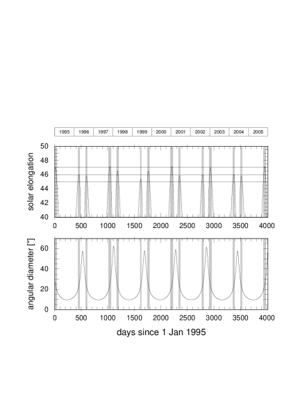
Figure 2: Observing constraints for Venus from 1995 to 2005. Shaded areas highlight the periods when the solar elongation of Venus exceeds $45\degr$, the minimum angle for a Chandra observation. The observing window in January 2001 was the most favourable one after the launch of Chandra.

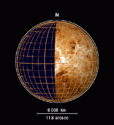
Figure 3: Viewing geometry of Venus during the ACIS–I observation on 13 Jan 2001. An equatorial grid $(\ell,b)$, with $\ell=0^{\circ}$ and $b=180^{\circ}$ marked by thick lines, is superimposed on a topographic map obtained by the Magellan mission. The dark area marks the geometrical shadow, and the outer white circle the extent of the model atmosphere.

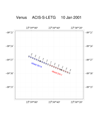
Figure 4: Venus during the LETG/ACIS–S observation on 10 Jan 2001, as seen from Chandra. The displacement from the geocentric position due to the parallax of the Chandra orbit varied between $2\farcm 1$ and $2\farcm 9$. This observation was split into two parts, to keep Venus in the ACIS–LETG field of view. Black dots show the two Chandra pointing directions. Images of the Venus crescent are plotted every 10 minutes. The size and orientation of Venus is drawn to scale.

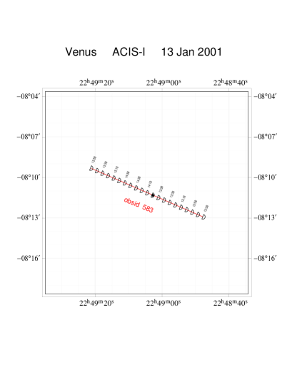
Figure 5: Same as Fig. 4, but for the ACIS–I observation on 13 Jan 2001. Here the parallactic displacement from the geocentric position varied between $2\farcm 6$ and $3\farcm 2$.

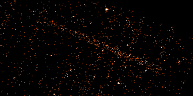
Figure 6: Venus moving across ACIS–I during the observation on 13 Jan 2001. Photons with Chandra standard grades, detected at $E<1\mbox{ keV}$, are displayed in celestial coordinates.

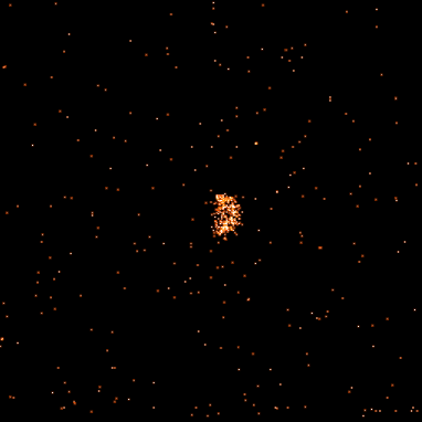
Figure 7: ACIS–I image of Venus in the (instrumental) energy range 0.2 – 1.0 keV, obtained after reprojecting the photons into the rest frame of Venus.

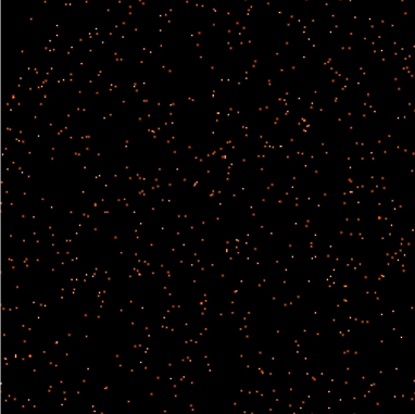
Figure 8: Same as Fig. 7, but for $E=$1.5 – 10 keV. No trace of Venus is visible.

At the time of the observation, Venus was moving across the sky with a proper motion of $2\farcm 6$/hour. As the CCDs were read out every 3.2 s, there was no need for continuous tracking. The spacecraft was oriented such that Venus would move parallel to one side of the CCDs and perpendicular to the dispersion direction in the LETG observation. To keep Venus well inside the $8\farcm 3$ field of view (FOV) of ACIS–S perpendicular to the dispersion direction, Chandra was repointed at the middle of the LETG / ACIS–S observation (Fig. 4, Tab. 1). For ACIS–I with its larger $16\farcm 9\times 16\farcm 9$ FOV, no repointing during the observation was necessary (Fig. 5, Tab. 1). As the photons were recorded time–tagged, an individual post–facto transformation into the rest frame of Venus was possible. This is illustrated in Figs. 6 and 7. The fact that all observations were performed with CCDs with intrinsic energy resolution made it possible to suppress the background with high efficiency (cf. Fig. 7 $\leftrightarrow\,$8 and Fig. 10, b $\leftrightarrow$ c).

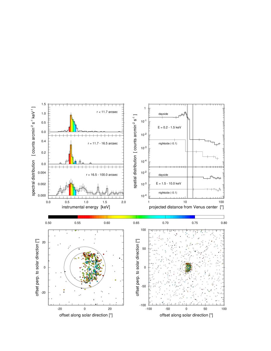
Figure 9: Summary of the ACIS–I observation. The frames at bottom show the distribution of photons around Venus in two different scales. Photons in the instrumental energy range 0.55 – 0.75 keV are highlighted by larger dots, filled with the color indicated above, while photons of 0.20 – 0.55 keV and 0.75 – 15.7 keV are plotted as black and white dots, respectively. In some cases the dots have been slightly shifted (by typically less than $1^{\prime\prime}$) to minimize overlaps. Two large circles are shown, the inner one, with $r=11\farcs 7$, indicating the geometric size of Venus, and the outer one, with $r=16\farcs 5$, enclosing practically all photons detected from Venus. The frames at upper left show the energy spectra observed for the three areas. The spectra of the two inner regions peak around 0.6 keV, with a tendency towards higher/lower energies in the inner/outer region. This behaviour is most likely caused by optical loading, a superposition of 0.53 keV photons and optical photons. The spectrum of the outermost region, i.e., the area of $200^{\prime\prime}\times 200^{\prime\prime}$ outside the outer ($r=16\farcs 5$) circle, shows no evidence for line emission. The histograms at upper right show the spatial distribution of the photons in the soft ($E=0.2$ – 1.5 keV) and hard ($E=1.5$ – 10.0 keV) energy range, in terms of surface brightness along radial rings around Venus, separately for the ‘dayside’ (offset along solar direction $>0$) and the ‘nightside’ (offset $<0$). For better clarity the nightside histograms were shifted by one decade downward. The bin size was adaptively determined so that each bin contains at least 24 counts. Thick vertical lines mark the radii of $11\farcs 7$ and $16\farcs 5$.

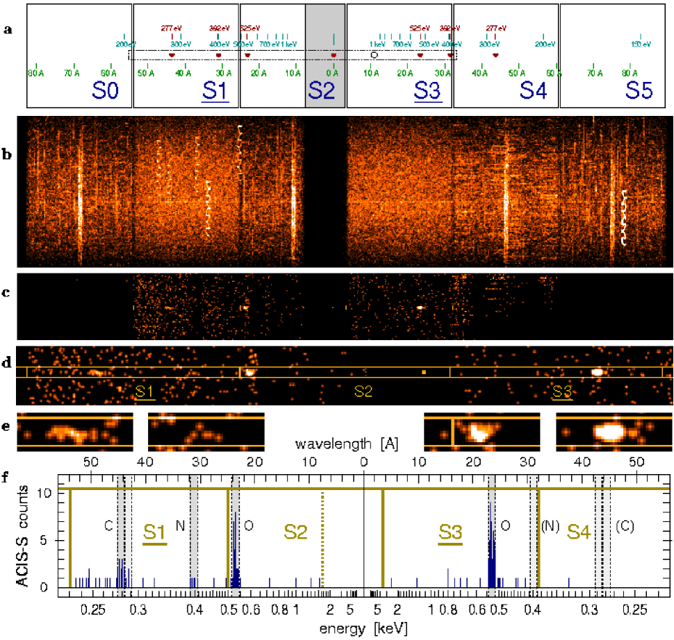
Figure 10: a) Expected LETG spectrum of Venus on the ACIS–S array. S1 and S3 are back–illuminated CCDs with increased sensitivity at low energies (underlined), while the others are front–illuminated. The nominal aimpoint, in S3, is marked with a circle. The aimpoint was shifted by $3\farcm 25$ into S2, to get more of the fluorescence lines covered by back–illuminated CCDs. Energy and wavelength scales are given along the dispersion direction. During the two pointings, Venus was moving perpendicularly to the dispersion direction. In order to avoid saturation of telemetry due to optical light, the shaded area around the zero order image in S2 was not transmitted. Images of Venus are drawn at the position of the C, N, and O fluorescence lines, with the correct size and orientation. The dashed rectangle indicates the section of the observed spectrum shown below. b) Distribution of all events with standard grades from the first ACIS–S pointing (obsid 2411), remapped into a coordinate system comoving with Venus, with the Sun at bottom. The events were binned into $2\farcs 5$ pixels. The white vertical curves are the trails of bright pixels, caused by a superposition of the Lissajous pattern of the satellite attitude and the apparent motion of Venus. The faint signal from Venus is lost in the noise. c) Central section of (b), after excluding bright pixels, and using the intrinsic resolution of ACIS for selecting only photons in the appropriate energy range. The two bright crescents symmetric to the center are images of Venus in the line of the O–K_α fluorescence emission, while the elongated enhancement at left is at the position of the C–K_α fluorescence emission line. The position of the zero order image (not transmitted) is indicated by a dot in S2. d, e) Enlargements of (c). f) Spectral scan along the region outlined in (d). Scales are given in keV and Å. The observed C, N, and O fluorescence emission lines are enclosed by dashed lines; the width of these intervals matches the size of the Venus crescent ($22\farcs 8$).

3 Results

The ACIS–I data clearly show that the X–ray spectrum of Venus is very soft: at energies $E>1.5\mbox{ keV}$ no enhancement is seen at the position of Venus, neither in the image (Fig. 8) nor in the surface brightness profile (Fig. 9). We determine a $3\,\sigma$ upper limit of $2.5\cdot 10^{-4}\mbox{ counts/s}$ to any flux from Venus in the 1.5 – 2.0 keV energy range. The corresponding value for $E=2$ – 8 keV is $5.6\cdot 10^{-4}\mbox{ counts/s}$. Further spectral analysis of the ACIS–I data is complicated by the presence of optical loading (Fig. 9).

The LETG spectrum, however, which is completely uncontaminated by optical light, clearly shows that most of the observed flux comes from O–K_α fluorescence (Fig. 10). As this flux is monochromatic, images of the Venus crescent (illuminated from bottom) show up along the dispersion direction. In addition to the O–K_α emission, we detect also fluorescence emission from C–K_α and, marginally, from N–K_α. The C–K_α image appears elongated, and spectral fits indicate the presence of an additional emission line at 0.29 keV, which might be the signature of the C $1s\to\pi^{\star}$ transition in CO₂ and CO.

Compared to its optical flux $f_{\rm opt}$, the total X–ray flux $f_{\rm x}$ from Venus is extremely low: $f_{\rm x}=2\cdot 10^{-10}\,f_{\rm opt}$. Taking into account that the energy of a K_α photon exceeds that of an optical photon by two orders of magnitude, we find that on average there is only one X–ray photon among $5\cdot 10^{11}$ photons from Venus. This extremely small fraction of X–ray versus optical flux, combined with the soft X–ray spectrum and the proximity of Venus to the Sun, illustrates the challenge of observing Venus in X–rays. The X–ray flux is emitted in just three narrow emission lines. Outside these lines the $f_{\rm x}/f_{\rm opt}$ ratio is even orders of magnitude lower.

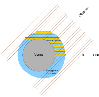
Figure 11: Modeling the X–ray appearance of Venus due to fluorescent scattering of solar X–rays. In the first step, the incident solar spectrum is computed for atmospheric columns which are parallel to the solar direction. The calculation starts at the top of the column and propagates towards the surface, taking the increasing attenuation into account. The absorbed flux is then converted into volume emissivities due to C, N, and O fluorescence. By sampling the emissivities in the volume elements along the line of sight, starting from the volume element which is farthest away from the observer, and taking the attenuation of this radiation due to subsequent photoabsorption along the line of sight into account, images of Venus can be obtained in the three fluorescence energies.

In the X–ray image (Fig. 7) the crescent of Venus is clearly resolved and allows detailed comparisons with the optical appearance. An optical image (Fig. 16 e), taken at the same phase angle, shows a sphere which is slightly more than half illuminated, closely resembling the geometric illumination (Fig. 3), with the brightness maximum well inside the crescent. In the X–ray image the sphere appears to be less than half illuminated. The most striking difference, however, is the pronounced limb brightening, which is particularly obvious in the surface brightness profiles (Fig. 9) and in the smoothed X–ray image (Fig. 16 d).

For a quantitative understanding of this brightening we performed a numerical simulation of the appearance of Venus in soft X–rays, based on fluorescent scattering of solar X–ray radiation (Fig. 11). The ingredients to this simulation were the composition and density structure of the Venus atmosphere (Fig. 12a), the photoabsorption cross sections (Fig. 13) and fluorescence efficiencies of the major atmospheric constituents, and the incident solar spectrum (Fig. 14). The simulation showed that the volume emissivity peaks at heights of 120 – 140 km and extends into the tenuous, optically thin parts of the thermosphere and exosphere (Fig. 12b). We see the volume emissivities accumulated along the line of sight without considerable absorption (Fig. 15), so that the observed brightness is mainly determined by the extent of the atmospheric column along the line of sight. This causes the pronounced brightening at the sunward limb, accompanied by reduced brightness at the terminator. Limb brightening would also be observed at other phase angles (Fig. 17).

The simulation shows that the amount of limb brightening is different for the three fluorescence energies (Fig. 16 a – c) and depends on the properties of the Venus atmosphere at heights above 110 km. Thus, information about the chemical composition and density structure of the Venus thermosphere and exosphere can be obtained by measuring the X–ray brightness distribution across the planet in the individual K_α fluorescence lines. This opens the possibility of using X–ray observations for remotely monitoring the properties of these regions in the Venus atmosphere which are difficult to investigate otherwise, and their response to solar activity.

Figure 12: a) Number density $n_{\rm CNO}=n_{\rm C}+n_{\rm N}+n_{\rm O}$ of the sum of C, N, and O atoms in the Venus model atmosphere as a function of the height above the surface. Between 60 and 100 km, the density shows a slight dependence on latitude. Above 110 km, the density depends considerably on the solar zenith angle (sza). b) Volume emissivities of C, N, and O K_α fluorescence photons at zenith angles of zero (subsolar, solid lines) and $90\degr$ (terminator, dashed lines) for the incident solar spectrum of Fig. 14. The height of maximum emissivity rises with increasing solar zenith angles because of increased path length and absorption along oblique solar incidence angles. In all cases maximum emissivity occurs in the thermosphere, where the optical depth depends also on the solar zenith angle.

Figure 13: Photoabsorption cross sections $\sigma_{\rm C}$, $\sigma_{\rm N}$, $\sigma_{\rm O}$ for C, N, and O (dashed lines), and $\sigma_{\rm CNO}$ for the chemical composition of the Venus atmosphere (solid line).

Figure 14: Incident solar X–ray photon flux on top of the Venus atmosphere ($h>180\mbox{ km}$) and at 114 km height (along subsolar direction). The spectrum is plotted with a bin size of 1 eV, which we used for the simulation in order to preserve the spectral details. At 114 km, it is considerably attenuated just above the K absorption edges, recovering towards higher energies.

Figure 15: Optical depth $\tau_{\rm CNO}=\tau_{\rm C}+\tau_{\rm N}+\tau_{\rm O}$ of the Venus model atmosphere with respect to CNO photoabsorption, as seen from outside. The upper/lower boundaries of the hatched area refer to energies just above/below the C and O edges (cf. Fig. 13). For better clarity the dependence on the solar zenith angle (sza) is only shown for $E=5.0\mbox{ keV}$; the curves for the other energies refer to $\mbox{sza}<50^{\circ}$. The dashed line, at $\tau=1$, marks the transition between the transparent ($\tau<1$) and opaque ($\tau>1$) range. For a specific energy, the optical depth increases by at least 13 orders of magnitude between 180 km and the surface. For comparison, the collisional depth resulting from charge exchange interactions with highly ionized atoms in the solar wind is also shown, for which a constant cross section of $3\cdot 10^{-15}\mbox{ cm}^{2}$ was assumed. Due to this large cross section, the tenuous exosphere of Venus is already collisionally thick. The flux of highly charged heavy solar wind ions, however, is too small to contribute significantly to the X–ray flux from Venus.

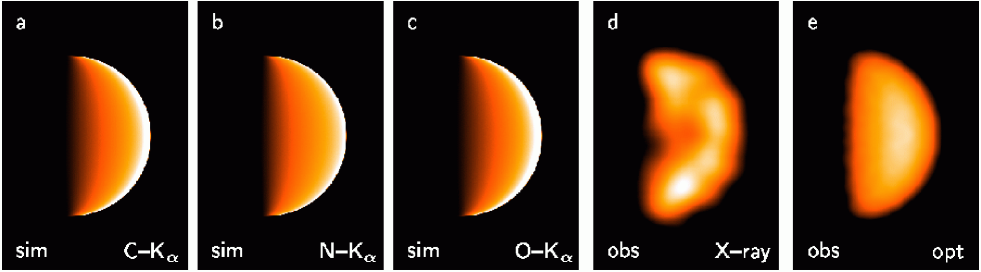
Figure 16: a – c) Simulated X–ray images of Venus at C–K_α, N–K_α, and O–K_α, for a phase angle of $86.5^{\circ}$. The X–ray flux is coded in a linear scale, extending from zero (black) to $1.2\cdot 10^{6}\mbox{ ph cm}^{-2}\mbox{ s}^{-1}$ (a), $5.2\cdot 10^{4}\mbox{ ph cm}^{-2}\mbox{ s}^{-1}$ (b), and $1.6\cdot 10^{6}\mbox{ ph cm}^{-2}\mbox{ s}^{-1}$ (c), (white). All images show considerable limb brightening, especially at C–K_α and O–K_α. d) Observed X–ray image: same as Fig. 1, but smoothed with a Gaussian filter with $\sigma=1\farcs 8$ and displayed in the same scale as the simulated images. This image is dominated by O–K_α fluorescence photons. e) Optical image of Venus, taken by one of the authors (KD) with a $4^{\prime\prime}$ Newton reflector on 2001 Jan 12.72 UT, 20 hours before the ACIS–I observation (cf. Tab. 1).

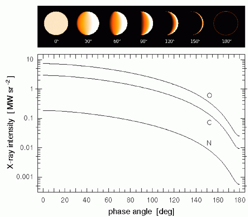
Figure 17: X–ray intensity of Venus as a function of phase angle, in the fluorescence lines of C, N, and O. The images at top, all displayed in the same intensity coding, illustrate the appearance of Venus at O–K_α for selected phase angles.

References

[\astronciteDennerl2002]
Dennerl, K., Burwitz, V., Englhauser, J., Lisse, C., Wolk, S. 2002,
A&A 386, 319 – 330