Studying large-scale structure with the 2dF Galaxy Redshift Survey

Abstract

The 2dF Galaxy Redshift Survey is the first to observe more than 100,000 redshifts. This allows precise measurements of many of the key statistics of galaxy clustering, in particular redshift-space distortions and the large-scale power spectrum. This paper presents the current 2dFGRS results in these areas. Redshift-space distortions are detected with a high degree of significance, confirming the detailed Kaiser distortion from large-scale infall velocities, and measuring the distortion parameter $\beta\equiv\Omega_{m}^{0.6}/b=0.43\pm 0.07$. The power spectrum is measured to $\mathrel{\lower 2.58334pt\hbox{$\buildrel{\textstyle<}\over{\scriptstyle\sim}$}}10\%$ accuracy for $k>0.02{\,h\,\rm Mpc^{-1}}$, and is well fitted by a CDM model with $\Omega_{m}h=0.20\pm 0.03$ and a baryon fraction of $0.15\pm 0.07$. A joint analysis with CMB data requires $\Omega_{m}=0.29\pm 0.05$, assuming scalar fluctuations, but no priors on other parameters. Two methods are used to determine the large-scale bias parameter: an internal bispectrum analysis yields $b=1.04\pm 0.11$, in very good agreement with the $b=1.10\pm 0.08$ obtained from a joint 2dFGRS+CMB analysis, again assuming scalar fluctuations. These figures refer to galaxies of approximate luminosity $2L^{*}$; luminosity dependence of clustering is detected at high significance, and is well described by $b/b^{*}=0.85+0.15(L/L^{*})$.

Institute for Astronomy, University of Edinburgh,
Royal Observatory, Edinburgh EH9 3HJ, UK

1. Aims and design of the 2dFGRS

The large-scale structure in the galaxy distribution is widely seen as one of the most important relics from an early stage of evolution of the universe. The 2dF Galaxy Redshift Survey (2dFGRS) was designed to build on previous studies of this structure, with the following main aims:

(1)      To measure the galaxy power spectrum $P(k)$ on scales up to a few hundred Mpc, bridging the gap between the scales of nonlinear structure and measurements from the the cosmic microwave background (CMB).

(2)      To measure the redshift-space distortion of the large-scale clustering that results from the peculiar velocity field produced by the mass distribution.

(3)      To measure higher-order clustering statistics in order to understand biased galaxy formation, and to test whether the galaxy distribution on large scales is a Gaussian random field.

The survey is designed around the 2dF multi-fibre spectrograph on the Anglo-Australian Telescope, which is capable of observing up to 400 objects simultaneously over a 2 degree diameter field of view. For details of the instrument and its performance see http://www.aao.gov.au/2df/, and also Lewis et al. (2002).

The source catalogue for the survey is a revised and extended version of the APM galaxy catalogue (Maddox et al. 1990a,b,c); this includes over 5 million galaxies down to $b_{\rm\scriptscriptstyle J}=20.5$ in both north and south Galactic hemispheres over a region of almost $10^{4}\,{\rm deg}^{2}$ (bounded approximately by declination $\delta\leq+3^{\circ}$ and Galactic latitude $b\mathrel{\lower 2.58334pt\hbox{$\buildrel{\textstyle>}\over{\scriptstyle\sim}$}}20^{\circ}$). This catalogue is based on Automated Plate Measuring machine (APM) scans of 390 plates from the UK Schmidt Telescope (UKST) Southern Sky Survey. The $b_{\rm\scriptscriptstyle J}$ magnitude system for the Southern Sky Survey is defined by the response of Kodak IIIaJ emulsion in combination with a GG395 filter, and is related to the Johnson–Cousins system by $b_{\rm\scriptscriptstyle J}=B-0.28(B-V)$. The photometry of the catalogue is calibrated with numerous CCD sequences and has a precision of approximately 0.15 mag for galaxies with $b_{\rm\scriptscriptstyle J}=17$–19.5. The star-galaxy separation is as described in Maddox et al. (1990b), supplemented by visual validation of each galaxy image.

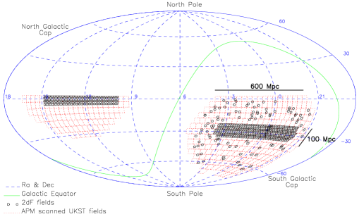
Figure 1.: The 2dFGRS fields (small circles) superimposed on the APM catalogue area (dotted outlines of Sky Survey plates). There are approximately 140,000 galaxies in the $75^{\circ}\times 15^{\circ}$ southern strip centred on the SGP, 70,000 galaxies in the $75^{\circ}\times 7.5^{\circ}$ equatorial strip, and 40,000 galaxies in the 100 randomly-distributed 2dF fields covering the whole area of the APM catalogue in the south.

The survey geometry is shown in Figure 1, and consists of two contiguous declination strips, plus 100 random 2-degree fields. One strip is in the southern Galactic hemisphere and covers approximately 75^∘$\times$15^∘ centred close to the SGP at ($\alpha,\delta$)=($01^{h}$,$-30^{\circ}$); the other strip is in the northern Galactic hemisphere and covers $75^{\circ}\times 7.5^{\circ}$ centred at ($\alpha,\delta$)=($12.5^{h}$,$+0^{\circ}$). The 100 random fields are spread uniformly over the 7000 deg² region of the APM catalogue in the southern Galactic hemisphere. At the median redshift of the survey ($\bar{z}=0.11$), $100{\,h^{-1}\,\rm Mpc}$ subtends about 20 degrees, so the two strips are $375{\,h^{-1}\,\rm Mpc}$ long and have widths of $75{\,h^{-1}\,\rm Mpc}$ (south) and $37.5{\,h^{-1}\,\rm Mpc}$ (north).

The sample is limited to be brighter than an extinction-corrected magnitude of $b_{\rm\scriptscriptstyle J}=19.45$ (using the extinction maps of Schlegel et al. 1998). This limit gives a good match between the density on the sky of galaxies and 2dF fibres. Due to clustering, however, the number in a given field varies considerably. To make efficient use of 2dF, we employ an adaptive tiling algorithm to cover the survey area with the minimum number of 2dF fields. With this algorithm we are able to achieve a 93% sampling rate with on average fewer than 5% wasted fibres per field. Over the whole area of the survey there are in excess of 250,000 galaxies.

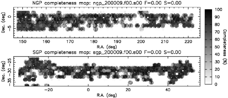
Figure 2.: The completeness as a function of position on the sky, as at January 2000. The circles are individual 2dF fields (‘tiles’). Unobserved tiles result in low completeness in overlap regions. Rectangular holes are omitted regions around bright stars. The lack of a complete set of overlapping tiles means that the completeness relative to the parent survey varies by over a factor of 2. However, such variations in the effective mask can be allowed for in statistical analyses.

2. Survey Status

By the end of 2001, observations had been made of 866 fields, yielding redshifts and identifications for 224,851 galaxies, 13630 stars and 176 QSOs, at an overall completeness of 93%. The galaxy redshifts are assigned a quality flag from 1 to 5, where the probability of error is highest at low $Q$. Most analyses are restricted to $Q\geq 3$ galaxies, of which there are currently 213,703. Data-taking will continue in 2002, but concentrating on increasing the completeness of the existing survey zone; the total number of $Q\geq 3$ galaxies is expected to asymptote to about 230,000. An interim data release took place in July 2001, consisting of approximately 100,000 galaxies (see Colless et al. 2001 for details). A public release of the full photometric and spectroscopic database is scheduled for July 2003.

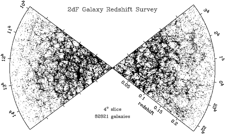
Figure 3.: The distribution of galaxies in part of the 2dFGRS, drawn from a total of 213,703 galaxies: slices $4^{\circ}$ thick, centred at declination $-2.5^{\circ}$ in the NGP and $-27.5^{\circ}$ in the SGP. This image reveals a wealth of detail, including linear supercluster features, often nearly perpendicular to the line of sight. The interesting question to settle statistically is whether such transverse features have been enhanced by infall velocities.

The Colless et al. (2001) paper details the practical steps that are necessary in order to work with a survey of this sort. The 2dFGRS does not consist of a simple region sampled with 100% efficiency, and it is therefore necessary to use a number of masks in order to interpret the data. Two of these concern the input catalogue: the boundaries of this catalogue, including ‘drilled’ regions around bright stars where galaxies could not be detected; also, revisions to the photometric calibration mean that in practice the survey depth varies slightly with position on the sky. The most important mask, however, arises from the way in which the sky is tessellated into 2dF tiles. The adaptive tiling algorithm is efficient, and yields uniform sampling in the final survey. However, at any intermediate stage, missing overlaps mean that the sampling fraction has fluctuations, as illustrated in Figure 2. This variable sampling makes quantification of the large scale structure more difficult, particularly for any analysis requiring relatively uniform contiguous areas. However, the effective survey ‘mask’ can be measured precisely enough that it can be allowed for in low-order analyses of the galaxy distribution. Figure 2 shows the mask at an earlier stage of the survey, appropriate for some of the first 2dFGRS analyses. The final database will have a more uniform mask, but it will always be necessary to allow for these sampling nonuniformities.

Despite these issues, the 2dFGRS now yields a strikingly detailed and complete view of the galaxy distribution over large cosmological volumes. This is illustrated in Figure 3, which shows the projection of a subset of the galaxies in the northern and southern strips onto $(\alpha,z)$ slices. In contemplating this picture, it is worth remembering the decades of effort that have been invested in establishing the reality of large-scale structure. Mapping these structures clearly is without doubt a historically important intellectual step for the human race, and it is a privilege to contribute to this process.

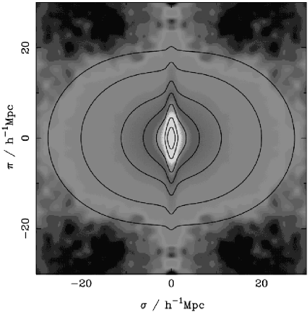
Figure 4.: The galaxy correlation function $\xi(\sigma,\pi)$ as a function of transverse ($\sigma$) and radial ($\pi$) pair separation is shown as a greyscale image. It was computed in $0.2{\,h^{-1}\,\rm Mpc}$ boxes and then smoothed with a Gaussian having an rms of $0.5{\,h^{-1}\,\rm Mpc}$. The contours are for a model with $\beta=0.4$ and $\sigma_{p}=400{\,\rm km\,s^{-1}}$, and are plotted at $\xi=10$, 5, 2, 1, 0.5, 0.2 and 0.1.

3. Redshift-space correlations

The simplest statistic for studying clustering in the galaxy distribution is the the two-point correlation function, $\xi(\sigma,\pi)$. This measures the excess probability over random of finding a pair of galaxies with a separation in the plane of the sky $\sigma$ and a line-of-sight separation $\pi$. Because the radial separation in redshift space includes the peculiar velocity as well as the spatial separation, $\xi(\sigma,\pi)$ will be anisotropic. On small scales the correlation function is extended in the radial direction due to the large peculiar velocities in non-linear structures such as groups and clusters – this is the well-known ‘Finger-of-God’ effect. On large scales it is compressed in the radial direction due to the coherent infall of galaxies onto mass concentrations – the Kaiser effect (Kaiser 1987).

To estimate $\xi(\sigma,\pi)$ we compare the observed count of galaxy pairs with the count estimated from a random distribution following the same selection function both on the sky and in redshift as the observed galaxies. We apply optimal weighting to minimise the uncertainties due to cosmic variance and Poisson noise. This is close to equal-volume weighting out to an adopted redshift limit of $z=0.25$. We have tested our results and found them to be robust against the uncertainties in both the survey mask and the weighting procedure. The redshift-space correlation function for the 2dFGRS computed in this way is shown in Figure 4. The correlation-function results display very clearly two signatures of redshift-space distortions. The ‘fingers of God’ from small-scale random velocities are very clear, as indeed has been the case from the first redshift surveys (e.g. Davis & Peebles 1983). However, this is the first time that the large-scale flattening from coherent infall has been seen in detail.

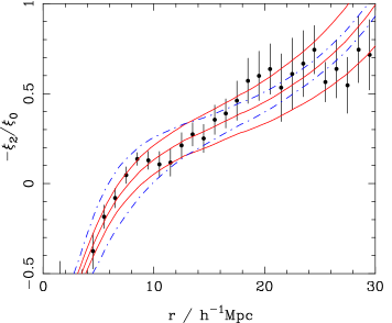
Figure 5.: (a) The compression of $\xi(\sigma,\pi)$ as measured by its quadrupole-to-monopole ratio, plotted as $-\xi_{2}/\xi_{0}$. The solid lines correspond to models with $\sigma_{p}=400{\,\rm km\,s^{-1}}$ and (bottom to top) $\beta=0.3$,0.4,0.5, while the dot-dash lines correspond to models with $\beta=0.4$ and (top to bottom) $\sigma_{p}=300,400,500{\,\rm km\,s^{-1}}$. (b) Likelihood contours for $\beta$ and $\sigma_{p}$ from the model fits. The inner contour is the one-parameter 68% confidence ellipse; the outer contours are the two-parameter 68%, 95% and 99% confidence ellipses. The central dot is the maximum likelihood fit, with $\beta=0.43$ and $\sigma_{p}=385{\,\rm km\,s^{-1}}$.

The degree of large-scale flattening is determined by the total mass density parameter, $\Omega_{m}$, and the biasing of the galaxy distribution. On large scales, it should be correct to assume a linear bias model, with correlation functions $\xi_{g}(r)=b^{2}\xi(r)$, so that the redshift-space distortion on large scales depends on the combination $\beta\equiv\Omega_{m}^{0.6}/b$. On these scales, linear distortions should also be applicable, so we expect to see the following quadrupole-to-monopole ratio in the correlation function:

$$\frac{\xi_{2}}{\xi_{0}}=\frac{3+n}{n}\frac{4\beta/3+4\beta^{2}/7}{1+2\beta/3+\beta^{2}/5}$$ (1)

(e.g. Hamilton 1992), where $n$ is the power spectrum index of the fluctuations, $\xi\propto r^{-(3+n)}$. This is modified by the Finger-of-God effect, which is significant even at large scales and dominant at small scales. The effect can be modelled by introducing a parameter $\sigma_{p}$, which represents the rms pairwise velocity dispersion of the galaxies in collapsed structures, $\sigma_{p}$ (see e.g. Ballinger et al. 1996). Full details of the fitting procedure are given in Peacock et al. (2001).

Figure 5a shows the variation in $\xi_{2}/\xi_{0}$ as a function of scale. The ratio is positive on small scales where the Finger-of-God effect dominates, and negative on large scales where the Kaiser effect dominates. The best-fitting model (considering only the quasi-linear regime with $8<r<25{\,h^{-1}\,\rm Mpc}$) has $\beta\simeq 0.4$ and $\sigma_{p}\simeq 400{\,\rm km\,s^{-1}}$; the likelihood contours are shown in Figure 5b. Marginalising over $\sigma_{p}$, the best estimate of $\beta$ and its 68% confidence interval is

$$\beta=0.43\pm 0.07$$ (2)

This is the first precise measurement of $\beta$ from redshift-space distortions; previous studies have shown the effect to exist (e.g. Hamilton, Tegmark & Padmanabhan 2000; Taylor et al. 2001; Outram, Hoyle & Shanks 2001), but achieved little more than 3$\sigma$ detections.

Our measurement of $\Omega^{0.6}/b$ would thus imply $\Omega=0.36\pm 0.10$ if $L^{*}$ galaxies are unbiased, but it is difficult to justify such an assumption in advance. We discuss below two methods by which the bias parameter may be inferred, which do in fact favour a low degree of bias. Nevertheless, there are other uncertainties in converting a measurement of $\beta$ to a figure for $\Omega$. The 2dFGRS has a median redshift of 0.11; with weighting, the mean redshift in the present analysis is $\bar{z}=0.17$, and our measurement should be interpreted as $\beta$ at that epoch. The optimal weighting also means that our mean luminosity is high: it is approximately 1.9 times the characteristic luminosity, $L^{*}$, of the overall galaxy population (Folkes et al. 1999; Madgwick et al. 2001). This means that we need to quantify the luminosity dependence of clustering.

4. Real-space clustering and its dependence on luminosity

The dependence of galaxy clustering on luminosity is an effect that was controversial for a number of years. Using the APM-Stromlo redshift survey, Loveday et al. (1995) claimed that there was no trend of clustering amplitude with luminosity, except possibly at the very lowest luminosities. In contradiction, the SSRS study of Benoist et al. (1996) suggested that the strength of galaxy clustering increased monotonically with luminosity, with a particularly marked effect for galaxies above $L^{*}$. The latter result was arguably more plausible, based on what we know of luminosity functions and morphological segregation. It has been clear for many years that elliptical galaxies display a higher correlation amplitude than spirals (Davis & Geller 1976). Since ellipticals are also more luminous on average, as shown most clearly by the 2dFGRS luminosity function results (Folkes et al. 1999; Madgwick et al. 2001), some trend with luminosity is to be expected, but the challenge is to detect it.

Figure 6.: (a) The correlation length in real space as a function of absolute magnitude. The solid line shows the predictions of the semi-analytic model of Benson et al. (2001), computed in a series of overlapping bins, each $0.5$ magnitudes wide. The dotted curves show an estimate of the errors on this prediction, including the relevant sample variance for the survey volume. (b) The real space correlation length estimated combining the NGP and SGP (filled circles). The open symbols show a selection of recent data from other studies.

The difficulty with measuring the dependence of $\xi(r)$ on luminosity is that cosmic variance can mask the signal of interest. It is therefore important to analyse volume-limited samples in which galaxies of different luminosities are compared in the same volume of space. This requires the rejection of many distant high-$L$ galaxies, and so the strategy is only feasible with a survey of the size of the 2dFGRS. This comparison was undertaken by Norberg et al. (2001a), who measured real-space correlation functions via the projection $\Xi(\sigma)=\int\xi(\sigma,\pi)\;d\pi$, demonstrating that it was possible to obtain consistent results in both NGP and SGP. A very clear detection of luminosity-dependent clustering was achieved, as shown in Figure 6. The results can be described by a linear dependence of effective bias parameter on luminosity:

$$b/b^{*}=0.85+0.15\,(L/L^{*}),$$ (3)

and the scale-length of the real-space correlation function for $L^{*}$ galaxies is approximately $r_{0}=4.8{\,h^{-1}\,\rm Mpc}$. There is thus a significant difference in the clustering amplitude of $L^{*}$ galaxies and the $L\simeq 1.9L^{*}$ characteristic of an optimally weighted sample, and this must be allowed for. This trend is in qualitative agreement with the results of Benoist et al. (1996), but in fact these workers gave a stronger dependence on luminosity than is indicated by the 2dFGRS. Finally, with spectral classifications, it is possible to measure the dependence of clustering both on luminosity and on spectral type, to see to what extent morphological segregation is responsible for this result. Norberg et al. (2001b) show that, in fact, the principal effect seems to be with luminosity: $\xi(r)$ increases with $L$ for all spectral types. This is reasonable from a theoretical point of view, in which the principal cause of different clustering amplitudes is the mass of halo that hosts a galaxy (e.g. Cole & Kaiser 1989; Mo & White 1996; Kauffman, Nusser & Steinmetz 1997).

5. The 2dFGRS power spectrum

Perhaps the key aim of the 2dFGRS was to perform an accurate measurement of the 3D clustering power spectrum, in order to improve on the APM result, which was deduced by deprojection of angular clustering (Baugh & Efstathiou 1993, 1994). The results of this direct estimation of the 3D power spectrum are shown in Figure 7. This power-spectrum estimate uses the FFT-based approach of Feldman, Kaiser & Peacock (1994), and needs to be interpreted with care. Firstly, it is a raw redshift-space estimate, so that the power beyond $k\simeq 0.2{\,h\,\rm Mpc^{-1}}$ is severely damped by fingers of God. On large scales, the power is enhanced, both by the Kaiser effect and by the luminosity-dependent clustering discussed above. Finally, the FKP estimator yields the true power convolved with the window function. This modifies the power significantly on large scales (roughly a 20% correction). We have made an approximate correction for this in Figure 7 by multiplying by the correction factor appropriate for a $\Gamma=0.25$ CDM spectrum. The precision of the power measurement appears to be encouragingly high, and the systematic corrections from the window are well specified.

Figure 7.: The 2dFGRS redshift-space dimensionless power spectrum, $\Delta^{2}(k)$, estimated according to the FKP procedure. The solid points with error bars show the power estimate. The window function correlates the results at different $k$ values, and also distorts the large-scale shape of the power spectrum An approximate correction for the latter effect has been applied. The solid and dashed lines show various CDM models, all assuming $n=1$. For the case with non-negligible baryon content, a big-bang nucleosynthesis value of $\Omega_{b}h^{2}=0.02$ is assumed, together with $h=0.7$. A good fit is clearly obtained for $\Omega_{m}h\simeq 0.2$. Note that the observed power at large $k$ will be boosted by nonlinear effects, but damped by small-scale random peculiar velocities. It appears that these two effects very nearly cancel, but model fitting is generally performed only at $k<0.15{\,h\,\rm Mpc^{-1}}$ in order to avoid these complications.

The next task is to perform a detailed fit of physical power spectra, taking full account of the window effects. The hope is that we will obtain not only a more precise measurement of the overall spectral shape, as parameterized by $\Gamma$, but will be able to move towards more detailed questions such as the existence of baryonic features in the matter spectrum (e.g. Meiksin, White & Peacock 1999). We summarize here results from the first attempt at this analysis (Percival et al. 2001).

In order to compare the 2dFGRS power spectrum to members of the CDM family of theoretical models, it is essential to have a proper understanding of the full covariance matrix of the data: the convolving effect of the window function causes the power at adjacent $k$ values to be correlated. This covariance matrix was estimated by applying the survey window to a library of Gaussian realisations of linear density fields for a $\Omega_{m}h=0.2$, $\Omega_{b}/\Omega_{m}=0.15$ CDM power spectrum, for which $\chi^{2}_{\rm min}=34.4$, given an expected value of $28$. The best fit power spectrum parameters are only weakly dependent on this choice. Similar results were obtained using a covariance matrix estimated from a set of mock catalogues derived from $N$-body simulations.

It is now possible to explore the space of CDM models, evaluating likelihood values assuming a Gaussian form for the likelihood. The likelihood contours in $\Omega_{b}/\Omega_{m}$ versus $\Omega_{m}h$ for this fit are shown in Figure 8. At each point in this surface we have marginalized by integrating the likelihood surface over the two free parameters, $h$ and the power spectrum amplitude. The result is not significantly altered if instead, the modal, or maximum mikelihood points in the plane corresponding to power spectrum amplitude and $h$ were chosen. The likelihood function is also dependent on the covariance matrix (which should be allowed to vary with cosmology), although the consistency of result from covariance matrices calculated for different cosmologies shows that this dependence is negligibly small. Assuming a uniform prior for $h$ over a factor of 2 is arguably over-cautious, and we have therefore added a Gaussian prior $h=0.7\pm 10\%$. This corresponds to multiplying by the likelihood from external constraints such as the HST key project (Freedman et al. 2001); this has only a minor effect on the results.

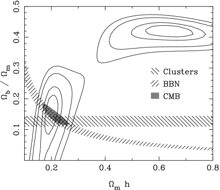
Figure 8.: Likelihood contours for the best-fit linear power spectrum over the region $0.02<k<0.15$. The normalization is a free parameter to account for the unknown large scale biasing. Contours are plotted at the usual positions for one-parameter confidence of 68%, and two-parameter confidence of 68%, 95% and 99% (i.e. $-2\ln({\cal L}/{\cal L_{\rm max}})=1,2.3,6.0,9.2$). We have marginalized over the missing free parameters ($h$ and the power spectrum amplitude) by integrating under the Likelihood surface. A prior on $h$ of $h=0.7\pm 10\%$ was assumed. This result is compared to estimates from x-ray cluster analysis (Evrard 1997), big-bang nucleosynthesis (Burles et al. 2001) and recent CMB results (Netterfield et al. 2001; Pryke et al. 2002). The CMB results assume that $\Omega_{b}h^{2}$ and $\Omega_{\rm cdm}h^{2}$ were independently determined from the data.

Figure 8 shows that there is a degeneracy between $\Omega_{m}h$ and the baryonic fraction $\Omega_{b}/\Omega_{m}$. However, there are two local maxima in the likelihood, one with $\Omega_{m}h\simeq 0.2$ and $\sim 20\%$ baryons, plus a secondary solution $\Omega_{m}h\simeq 0.6$ and $\sim 40\%$ baryons. The high-density model can be rejected through a variety of arguments, and the preferred solution is

$$\Omega_{m}h=0.20\pm 0.03;\quad\quad\Omega_{b}/\Omega_{m}=0.15\pm 0.07.$$ (4)

The 2dFGRS data are compared to the best-fit linear power spectra convolved with the window function in Figure 9. This shows where the two branches of solutions come from: the low-density model fits the overall shape of the spectrum with relatively small ‘wiggles’, while the solution at $\Omega_{m}h\simeq 0.6$ provides a better fit to the bump at $k\simeq 0.065{\,h\,\rm Mpc^{-1}}$, but fits the overall shape less well.

Figure 9.: The 2dFGRS data compared with the two preferred models from the Maximum Likelihood fits convolved with the window function (solid lines). Error bars show the diagonal elements of the covariance matrix, for the fitted data that lie between the dotted vertical lines. The unconvolved models are also shown (dashed lines). The $\Omega_{m}h\simeq 0.6$, $\Omega_{b}/\Omega_{m}=0.42$, $h=0.7$ model has the higher bump at $k\simeq 0.05{\,h\,\rm Mpc^{-1}}$. The smoother $\Omega_{m}h\simeq 0.20$, $\Omega_{b}/\Omega_{m}=0.15$, $h=0.7$ model is a better fit to the data because of the overall shape.

It is interesting to compare these conclusions with other constraints. These are shown on Figure 8, assuming $h=0.7\pm 10\%$. Latest estimates of the Deuterium to Hydrogen ratio in QSO spectra combined with big-bang nucleosynthesis theory predict $\Omega_{b}h^{2}=0.020\pm 0.001$ (Burles et al. 2001), which translates to the shown locus of $f_{\rm\scriptscriptstyle B}$ vs $\Omega_{m}h$. X-ray cluster analysis predicts a baryon fraction $\Omega_{b}/\Omega_{m}=0.127\pm 0.017$ (Evrard 1997) which is within $1\sigma$ of our value. These loci intersect very close to our preferred model. Moreover, these results are in good agreement with independent estimates of the total density and baryon content from the latest data on CMB anisotropies (Netterfield et al. 2001; Pryke et al. 2002). For scalar-only models, these favour CDM and baryon physical densities of $\Omega_{c}h^{2}=0.15\pm 0.03$ and $\Omega_{b}h^{2}=0.0215\pm 0.0025$. If we take $h=0.7\pm 10\%$, this gives

$$\Omega_{m}h=0.21\pm 0.05;\quad\quad\Omega_{b}/\Omega_{m}=0.14\pm 0.03,$$ (5)

in remarkably good agreement with the estimate from the 2dFGRS

$$\Omega_{m}h=0.20\pm 0.03;\quad\quad\Omega_{b}/\Omega_{m}=0.15\pm 0.07.$$ (6)

Perhaps the main point to emphasise here is that the 2dFGRS results are not greatly sensitive to the assumed tilt of the primordial spectrum. We have used CMB results to motivate the choice of $n=1$, as discussed below, but it is clear that very substantial tilts are required to alter the conclusions significantly: $n\simeq 0.8$ would be required to turn zero baryons into the preferred model. The dependence on tilt emphasises that the baryon signal comes in good part from the overall shape of the spectrum. Although the eye is struck by a single sharp ‘spike’ at $k\simeq 0.065{\,h\,\rm Mpc^{-1}}$, the correlated nature of the errors in the $P(k)$ estimate means that such features tend not to be significant in isolation. We note that the convolving effects of the window would require a very substantial spike in the true power in order to match our data exactly. This is not possible within the compass of conventional models, and the conservative conclusion is that the apparent spike is probably enhanced by correlated noise. A proper statistical treatment is essential in such cases.

6. Combination with the CMB and cosmological parameters

The 2dFGRS power spectrum contains important information about the key parameters of the cosmological model, but we have seen that additional assumptions are needed, in particular the values of $n$ and $h$. Observations of CMB anisotropies can in principle measure most of the cosmological parameters, and combination with the 2dFGRS can lift most of the degeneracies inherent in the CMB-only analysis. It is therefore of interest to see what emerges from a joint analysis.

These issues are discussed in Efstathiou et al. (2002), and in Efstathiou’s presentation at this meeting. The CMB data alone contain two important degeneracies: the ‘geometrical’ and ‘tensor’ degeneracies. In the former case, one can evade the commonly-stated CMB conclusion that the universe is flat, by adjusting both $\Lambda$ and $h$ to extreme values. In the latter case, a model with a large tensor component can be made to resemble a zero-tensor model with large blue tilt ($n>1$) and high baryon content. Efstathiou et al. (2002) show that adding the 2dFGRS data removes the first degeneracy, but not the second. This is reasonable: if we take the view that the CMB determines the physical density $\Omega_{m}h^{2}$, then a measurement of $\Omega_{m}h$ from 2dFGRS gives both $\Omega_{m}$ and $h$ separately in principle, removing one of the degrees of freedom on which the geometrical degeneracy depends. On the other hand, the 2dFGRS alone constrains the baryon content weakly, so this does not remove the scope for the tensor degeneracy.

On the basis of this analysis, we can therefore be confident that the universe is very nearly flat, so it is defensible to assume hereafter that this is exactly true. The importance of tensors will of course be one of the key questions for cosmology over the next several years, but it is interesting to consider the limit in which these are negligible. In this case, the standard model for structure formation contains a vector of only 6 parameters:

$${\bf p}=(n_{s},\Omega_{m},\Omega_{b},h,Q,\tau).$$ (7)

Of these, the optical depth to last scattering, $\tau$, is almost entirely degenerate with the normalization, $Q$ – and indeed with the bias parameter; we discuss this below. The remaining four parameters are pinned down very precisely, as shown in Figure 10. Using the latest CMB data, including COBE (Wright et al. 1996), Boomerang (Netterfield et al. 2001, de Bernardis et al. 2002), Maxima (Lee et al. 2001; Stomper et al. 2001) and DASI (Halverson et al. 2002; Pryke et al. 2002), plus the 2dFRGS power spectrum, we obtain

$$(n_{s},\Omega_{c}h^{2},\Omega_{b}h^{2},h)=(1.00\pm 0.05,0.114\pm 0.009,0.022\pm 0.002,0.68\pm 0.05),$$ (8)

or an overall density parameter of $\Omega_{m}=0.29\pm 0.05$.

It is remarkable how well these figures agree with completely independent determinations: $h=0.72\pm 0.08$ from the HST key project (Mould et al. 2000; Freedman et al. 2001); $\Omega_{b}h^{2}=0.020\pm 0.001$ (Burles et al. 2001). This gives confidence that the tensor component must indeed be sub-dominant.

Figure 10.: Likelihood contours for a fit to current CMB data plus the 2dFGRS power spectrum, assuming flat scalar-dominated models. With these assumptions, there are no significant parameter degeneracies, and the optimal model is well specified. Impressively, the required values for the Hubble parameter and baryon density are in very good agreement with direct estimates, although no prior information on these parameters was included.

7. The degree of bias

7.1. Bispectrum

Another key issue which we can address with these results is the extent to which the galaxy distribution is biased. As far as the large-scale results on the power spectrum are concerned, there is a degeneracy between the unknown amplitude of the matter power spectrum $P(k)$ and the degree of bias, $b$, defined such that the galaxy power spectrum is $P_{g}(k)\equiv b^{2}P(k)$. At later times (or on smaller scales), this degeneracy is lifted by nonlinear effects. One feature of nonlinear gravitational evolution is that the overdensity field becomes progressively more skewed towards high density (assuming Gaussian initial fluctuations). One could hope to exploit this gravitational skewness, but skewness could equally well arise from biasing, e.g. from a galaxy formation efficiency that increased at dense points in the mass field. It is nevertheless possible to distinguish these two effects by considering the shapes of isodensity regions. If the field is unbiased, then the shapes of isodensity contours become flattened, as gravitational instability accelerates collapse along the short axis of structures, leading to sheet-like and filamentary structures.

Figure 11.: $b_{1}$ recovered with the bispectrum method versus the underlying (true) $b_{1}\equiv(P_{g}/P_{m})^{1/2}$ for 16 mock SGP simulations for the $\tau$CDM (open circles) and $\Lambda$CDM (solid circles) models. Note that the 2dFGRS has data in the NGP and SGP, reducing the error bar compared to these mock catalogues. Even so, it is clear that the bispectrum method can discriminate between strongly biased $\Omega=1$ models and relatively unbiased models such as $\Lambda$CDM.

In Verde et al. (2001), this effect is studied using the bispectrum $B$, which is related to the three-point correlation function in Fourier space. For the mass, this is defined by

$$\langle\delta_{{\bf k}_{1}}\delta_{{\bf k}_{2}}\delta_{{\bf k}_{3}}\rangle\equiv(2\pi)^{3}B({\bf k}_{1},{\bf k}_{2},{\bf k}_{3})\delta^{\rm D}({\bf k}_{1}+{\bf k}_{2}+{\bf k}_{3}),$$ (9)

where $\delta_{{\bf k}}\equiv\int d^{3}{\bf x}\,\delta({\bf x})\exp(-i{\bf k}\cdot{\bf x})$ is the Fourier transform of the mass overdensity and $\delta^{\rm D}$ is the Dirac delta function; this shows that the bispectrum can be non-zero only if the ${\bf k}$-vectors close to form a triangle.

For Gaussian fluctuations, the bispectrum is zero by symmetry, but it becomes non-zero under gravitational evolution, in the same way as a non-zero skewness develops. In lowest-order perturbation theory, Fourier coefficients develop a nonlinear component which is proportional to $\delta^{2}$, so the leading order term in the bispectrum grows like $\delta^{4}$. Since the 2dFGRS is not a survey of mass density, to interpret the bispectrum measured from the survey we must make some assumption about the distribution of mass relative to the distribution of galaxies. The simplest assumption is a bias that is a causal (but nonlinear) function of the mass density:

$$\delta_{g}=b_{0}+b_{1}\delta+b_{2}\delta^{2}/2+\dots$$ (10)

For consistency with perturbation theory, we must keep the quadratic bias term involving $b_{2}$; this induces a calculable constant offset $b_{0}$, since $\langle\delta_{g}\rangle\equiv 0$. This is a fairly general formulation, although it ignores stochastic effects (Dekel & Lahav 1999), and it is a form of local bias (modulo the smoothing scale used to define the quasilinear density field).

For practical estimation of the bispectrum, it is necessary to decide which triangles to consider. In practice, we use two sets of triangles of different configurations: one set with one wavevector twice the length of another, and another set with two wavevectors of common length. With a constraint of $k<0.35{\,h\,\rm Mpc^{-1}}$, this yields 80 million triangles. Results for mock data are shown in Figure 11, demonstrating that highly-biased models can be distinguished from nearly unbiased models. The mock samples also provide a direct estimate of the errors on the bias parameters, yielding the 2dFGRS results:

  $${b_{1}} {{}=1.04\pm 0.11} {b_{2}} {{}=-0.05\pm 0.08}$$   (11)

Remarkably, the simplest possible model works: there need be no segregation of mass and light on the largest scales. On smaller scales, we know that the nonlinear mass power spectrum has a shape that almost inevitably differs from that of the light (e.g. Seljak 2000; Peacock & Smith 2000), so light cannot trace mass exactly. Nevertheless, the degree of large-scale bias is small.

Again, this result is obtained using optimal weighting, so the value of $b_{1}=1.04\pm 0.11$ refers to $L\simeq 1.9L^{*}$ galaxies, as for the $\beta$ analysis. We can therefore combine these figures to estimate $\Omega_{m}$, obtaining $\Omega_{m}=0.27\pm 0.06$. Strictly, this refers to $\Omega_{m}$ at the effective redshift of 0.17; for a flat model, evolution to $z=0$ is significant, yielding $\Omega_{m}=0.19\pm 0.04$ – a result that is entirely internal to the 2dFGRS. This is smaller than the figure of $0.29\pm 0.05$ from the 2dFGRS+CMB analysis, but the two are consistent; the formal average of these two results is $\Omega_{m}=0.23\pm 0.03$.

7.2. Fluctuation amplitude from the CMB

An alternative and completely independent approach is to infer the degree of bias directly by using the amplitude of mass fluctuations inferred from the CMB. This analysis was performed by Lahav et al. (2001).

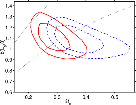
Figure 12.: The result of a joint likelihood fit to 2dFGRS+CMB. The marginalization (without any external priors) is over $h,\Omega_{b}h^{2}$ and $\sigma_{8{\rm m}}$. Other parameters are held fixed ($n=1,\tau=0$); results for $n=0.9$ are shown as dashed lines. The contours are for (two-parameter) 68 per cent and 95 per cent confidence intervals. The dotted lines represent a 1-$\sigma$ envelope for $\beta(L_{s},0)$, based on $\beta(L_{s},z_{s})=0.43\pm 0.07$ from Peacock et al. (2001) and the CGC model.

Given assumed values for the cosmological parameters, the present-day linear normalization of the mass spectrum (e.g. $\sigma_{8}$) can be inferred. It is convenient to define a corresponding measure for the galaxies, $\sigma_{8{\rm g}}$, such that we can express the bias parameter as

$$b={\sigma_{8{\rm g}}\over\sigma_{8{\rm m}}}.$$ (12)

In practice, we define $\sigma_{8{\rm g}}$ to be the value required to fit a CDM model to the power-spectrum data on linear scales ($0.02<k<0.15{\,h\,\rm Mpc^{-1}}$). A final necessary complication of the notation is that we need to distinguish between the apparent values of $\sigma_{8{\rm g}}$ as measured in redshift space ($\smash{\sigma_{8{\rm g}}^{S}}$) and the real-space value that would be measured in the absence of redshift-space distortions ($\smash{\sigma_{8{\rm g}}^{R}}$). It is the latter value that is required in order to estimate the bias.

A model grid covering the range $0.1<\Omega_{m}h<0.3$, $0.0<\Omega_{b}/\Omega_{m}<0.4$, $0.4<h<0.9$ and $0.75<\smash{\sigma^{S}_{8{\rm g}}}<1.14$ was considered. The primordial index was assumed to be $n=1$ initially, and the dependence on $n$ studied separately. For fixed ‘concordance model’ parameters $n=1$, $k=0$, $\Omega_{m}=0.3$, $\Omega_{b}h^{2}=0.02$ and a Hubble constant $h=0.70$, we find that the amplitude of 2dFGRS galaxies in redshift space is $\smash{\sigma_{8{\rm g}}^{S}}(L_{s},z_{s})=0.94$. Correcting for redshift-space distortions as detailed above reduces this to 0.86 in real space. Applying a correction for the mean luminosity of $1.9L^{*}$ using the recipe of Norberg et al. (2001a), we obtain an estimate of $\smash{\sigma_{8{\rm g}}^{R}}(L^{*},z_{s})=0.76$, with a negligibly small random error. In order to obtain present-day bias figures, we need to know the evolution of galaxy clustering to $z=0$. Existing data on clustering evolution reveals very slow changes: higher bias at early times largely cancels the evolution of the dark matter. We therefore assume no evolution in $\smash{\sigma_{8{\rm g}}}$: the CGC (constant galaxy clustering) model. This has the consequence that $b(z_{s})=1.09\,b(z=0)$.

One can now compare the galaxy figure with $\sigma_{8}$ for mass, deduced by fitting to the latest CMB data, as discussed above. In Figure 12, we show joint confidence intervals on the inferred linear bias parameter and $\Omega_{m}$. Marginalising over $\Omega_{m}$ gives an estimate for the linear bias parameter. This applies only for $n=1$ and negligible optical depth to last scattering, but it is simple to obtain an empirical correction for these effects:

$$b(L_{s},z=0)=(1.10\pm 0.08)\,\exp[-\tau+0.5(n-1)].$$ (13)

Thus, large $\tau$ requires antibias, as does a red tilt with $n<1$. From earlier results, the tilt effects are probably negligible. For BBN baryons plus a reionization redshift of 10, $\tau\simeq 0.07$. Very much larger values can probably be ruled out, as the bias inferred by this method would then disagree with the bispectrum calculation. Formally, taking $n=1$, we obtain $\tau<0.4$ at 95% confidence.

8. Conclusions

The 2dFGRS is the first 3D survey of the local universe to achieve 100,000 redshifts, almost an order of magnitude improvement on previous work. The final database should yield definitive results on a number of key issues relating to galaxy clustering. For details of the current status of the 2dFGRS, see http://www.mso.anu.edu.au/2dFGRS. In particular, this site gives details of the 2dFGRS public release policy, in which approximately the first half of the survey data were made available in June 2001, with the complete survey database to be made public by mid-2003. The key results of the survey to date may be summarized as follows:

(1)      The galaxy luminosity function has been measured precisely as a function of spectral type (Folkes et al. 1999; Madgwick et al. 2001).

(2)      The amplitude of galaxy clustering has been shown to depend on luminosity (Norberg et al. 2001a). The relative bias is $b/b^{*}=0.85+0.15\,(L/L^{*})$.

(3)      The redshift-space correlation function has been measured out to $30{\,h^{-1}\,\rm Mpc}$. Redshift-space distortions imply $\beta\equiv\Omega_{m}^{0.6}/b=0.43\pm 0.06$, for galaxies with $L\simeq 1.9L^{*}$.

(4)      The galaxy power spectrum has been measured to high accuracy (10–15% rms) over about a decade in scale at $k<0.15{\,h\,\rm Mpc^{-1}}$. The results are very well matched by an $n=1$ CDM model with $\Omega_{m}h=0.2$ and 15% baryons.

(5)      Combining the power spectrum results with current CMB data, very tight constraints are obtained on cosmological parameters. For a scalar-dominated flat model, we obtain $\Omega_{m}=0.29\pm 0.05$, $\Omega_{b}h^{2}=0.022\pm 0.002$ and $h=0.68\pm 0.04$, independent of external data.

(6)      Results from the CMB comparison imply a large-scale bias parameter consistent with unity. This conclusion is also reached in a completely independent way via the bispectrum analysis of Verde et al. (2001).

Overall, these results provide precise support for a cosmological model that is flat, with $(\Omega_{b},\Omega_{c},\Omega_{v})\simeq(0.04,0.25,0.71)$, to a tolerance of 10% in each figure. Although the $\Lambda$CDM model has been claimed to have problems in matching galaxy-scale observations, it clearly works extremely well on large scales, and any proposed replacement for CDM will have to maintain this agreement. So far, there has been no need to invoke either tilt of the scalar spectrum, or a tensor component in the CMB. If this situation is to change, the most likely route will be via new CMB data, combined with the key complementary information that the large-scale structure in the 2dFGRS can provide.

References

Ballinger W.E., Peacock J.A., Heavens A.F., 1996, MNRAS, 282, 877

Baugh C.M., Efstathiou G., 1993, MNRAS, 265, 145

Baugh C.M., Efstathiou G., 1994, MNRAS, 267, 323

Benoist C., Maurogordato S., da Costa L.N., Cappi A., Schaeffer R., 1996, ApJ, 472, 452

Benson, A.J., Frenk, C.S., Baugh, C.M., Cole, S., Lacey, C.G., 2001, MNRAS, 327, 1041

Burles S., Nollett K.M., Turner M.S., 2001, ApJ, 552, L1

Cole S., Kaiser N., 1989, MNRAS, 237, 1127

Colless M. et al., 2001, MNRAS, 328, 1039

Davis M., Geller M.J., 1976, ApJ, 208, 13

Davis M., Peebles, P.J.E., 1983, ApJ, 267, 465

de Bernardis P. et al., 2002, ApJ, 564, 559

Dekel A., Lahav O., 1999, ApJ, 520, 24

Efstathiou G. et al., 2002, MNRAS, 330, L29

Evrard A., 1997, MNRAS, 292, 289

Folkes S.J. et al., 1999, MNRAS, 308, 459

Feldman H.A., Kaiser N., Peacock J.A., 1994, ApJ, 426, 23

Freedman W.L. et al., 2001, ApJ, 553, 47

Halverson N.W. et al., 2002, ApJ, 568, 38

Hamilton A.J.S., 1992, ApJ, 385, L5

Hamilton A.J.S., Tegmark M., Padmanabhan N., 2000, MNRAS, 317, L23

Kaiser N., 1987, MNRAS, 227, 1

Lahav O. et al., 2001, astro-ph/0112162

Lee A.T. et al., 2001, ApJ, 561, L1

Lewis I.J. et al., 2002, MNRAS, in press, astro-ph/0202175

Loveday J., Maddox S.J., Efstathiou G., Peterson B.A., 1995, ApJ, 442, 457

Maddox S.J., Efstathiou G., Sutherland W.J., Loveday J., 1990a, MNRAS, 242, 43p

Maddox S.J., Sutherland W.J., Efstathiou G., Loveday J., 1990b, MNRAS, 243, 692

Maddox S.J., Efstathiou G., Sutherland W.J., 1990c, MNRAS, 246, 433

Madgwick D. et al., 2001, astro-ph/0107197

Meiksin A.A., White M., Peacock J.A., 1999, MNRAS, 304, 851

Mo H.J., White S.D.M., 1996, MNRAS, 282, 347

Mould J.R. et al., 2000, ApJ, 529, 786

Netterfield C.B. et al., 2001, astro-ph/0104460

Norberg P. et al., 2001a, MNRAS, 328, 64

Norberg P. et al., 2001b, astro-ph/0112043

Outram P.J., Hoyle F., Shanks T., 2001, MNRAS, 321, 497

Peacock J.A. et al., 2001, Nature, 410, 169

Peacock J.A., Smith R.E., 2000, MNRAS, 318, 1144

Percival W.J. et al., 2001, MNRAS, 327, 1297

Pryke C. et al., 2002, ApJ, 568, 46

Schlegel D.J., Finkbeiner D.P., Davis M., 1998, ApJ, 500, 525

Seljak U., 2000, MNRAS, 318, 203

Stompor R. et al., 2001, ApJ, 561, L7

Taylor A.N., Ballinger W.E., Heavens A.F., Tadros H., 2001, MNRAS, 327, 689

Verde L. et al., 2001, astro-ph/0112161

Wright E.L., Bennett C.L., Gorski K., Hinshaw G., Smoot G.F., 1996, ApJ, 464, L21