Vacuum gap model for PSR B0943$+$10

PSR B0943$+$10 is known to show remarkably stable drifting subpulses, which can be interpreted in terms of a circumferential motion of 20 sparks, each completing one circulation around the periphery of the polar cap in 37 pulsar periods. We use this observational constraint and argue that the vacuum gap model can adequately describe the observed drift patterns. Further we demonstrate that only the presence of strong non-dipolar surface magnetic field can favor such vacuum gap formation. Subsequently, for the first time we are able to constrain the parameters of the surface magnetic field, and model the expected magnetic structure on the polar cap of PSR B0943$+$10 considering the inverse Compton scattering photon dominated vacuum gap.

1 Introduction

The fundamental problem of pulsar research is lack of consensus about the radio emission mechanism, except that the electron-positron pair production is an essential ingredient, to explain the observed coherent radiation. Moreover, the observed phenomenon of drifting subpulses serves as an excellent diagnostic tool to investigate the mechanism of pulsar radio emission. PSR B0943+10 with period $P=1.09$ s and period derivative $\dot{P}=3.5\cdot 10^{-15}$ s/s exhibits long and stable sequences of drifting subpulses (Deshpande & Rankin 1999, 2001, hereafter DR99 and DR01, Asgekar & Deshpande 2001). This pulsar is observable only at frequencies below 800 MHz (high frequency radiation most probably misses the line-of-sight due to specific observing geometry) and drifting subpulses with similar features are observed at 35, 111 and 430 MHz, implying broad-band nature of the phenomenon. This suggests that drifting subpulses in this pulsar are associated with a stable system of emission subbeams, rotating around the pulsar magnetic axis. The aliasing resolved analysis of the harmonic-resolved fluctuation spectra related to drifting subpulses yielded in precise estimates of periodicities of phase and amplitude modulation, namely $P_{3}=1.87\leavevmode\nobreak\ P$ and $\hat{P}_{3}=37\leavevmode\nobreak\ P$, respectively (DR01). These two periodicities are harmonically related and are used to determine the number of subpulse beams $N=\hat{P}_{3}/P_{3}=20$ contributing to the observed modulations. The subpulse “drift-bands” clearly visible in the observed drift pattern (Backer 1973) are separated vertically by $\hat{P}_{3}$ (in pulsar periods) and horizontally by $P_{2}$ (in pulse longitude). The latter is estimated as being about $11^{\circ}$ and can be converted into the magnetic azimuth angle $\eta$ separating adjacent subbeams. This requires knowledge of the inclination angle $\alpha$ and the impact angle $\beta$, which for this pulsar is estimated from the polarization measurements and from the viewing geometry that leads to missing radiation above $\sim 800$ MHz. Using $\alpha=11^{\circ}.64$ and $\beta=-4.31^{\circ}$ (DR01), one gets $\eta=18^{\circ}$, which in turn gives $N=360^{\circ}/\eta=20$ subbeams rotating at the beam periphery of PSR B0943$+$10.

Karastergiou et al.(2001) observed simultaneously subpulses in single pulses of PSR B0329+34 at 1.4 and 2.7 GHz. Careful analysis of these observations suggests strongly that a single plasma column fed by a single entity at the bottom of the pulsar magnetosphere is responsible for the subpulse observed across the pulsar spectrum, which can be interpreted naturally in terms of sparks operating on the polar cap surface. This picture is probably more general and can be applied to other pulsars, including those with drifting subpulses. Deshpande & Rankin (1999) noticed that the subpulse drift phenomenon observed in PSR B0943$+$10 is consistent with the model proposed by Ruderman & Sutherland (1975, hereafter RS75), in which the subbeams are associated with sparking discharges operating within the vacuum gap (VG) developed just above the polar cap. The observed subpulse drift rate in this model arises from the speed of circulation of sparks around the magnetic axis, which is determined by rate of the ${\bf E}\times{\bf B}$ drift of electron-positron plasma confined to the isolated spark filament within the VG. If the planes of surface magnetic field lines are more or less perpendicular to the polar cap boundary, then the peripherial sparks will slowly rotate around the magnetic axis. Deshpande & Rankin (1999) demonstrated clearly that the non-corotating subbeams associated with drifting subpulses actually lag the stellar rotation. This finding strenghtens the VG plasma ${\bf E}\times{\bf B}$ drift hypothesis. However, the formation of VG itself suffered criticism owing to the problem of binding energy of ions, not being high enough to be retained on the stellar surface (Hillenbrandt & Müller 1976, Kössl et al 1988). Morover, the association of drifting subpulses with sparks was questioned based on the fact that sparks will move towards the magnetic pole at a speed much faster than the ${\bf E}\times{\bf B}$ drift velocity, thus quenching the stable drifting patterns (Cheng & Ruderman, 1977; Filippenko & Radhakrishnan, 1982). In this paper we demonstrate that indeed VG can form in PSR B0943$+$10 if the surface magnetic field is very strong and non-dipolar in nature. For the first time we are able to constrain the parameters of the surface magnetic field assuming that the VG is dominated by the inverse Compton scattering photons. We also demonstrate that the embarrassing problem with rapid spark motion towards the pole will not occur due to specific geometry of the surface magnetic field in the VG, at least in PSR B0943$+$10.

2 Constraining surface field in PSR B0943$+$10

2.1 Vacuum Gap formation

Gil & Mitra (2001, hereafter GM01) argued that VG can form in neutron stars with very strong non-dipolar surface magnetic field $B_{s}=b\cdot B_{d}$, where $B_{d}=2\cdot 10^{12}(P\cdot\dot{P}_{-15})^{0.5}$ G is the inferred dipolar field $(B_{d}=4\times 10^{12}$ G in this case) and $\dot{P}_{-15}=\dot{P}/10^{-15}$. For surface magnetic fields with $b\gg 1$, the radius of curvature of field lines ${\cal R}$ should be relatively small, with normalized values ${\cal R}_{6}={\cal R}/R<<100$, where $R=10^{6}$ cm is the neutron star radius. GM01 considered strong magnetic fields $B>0.1\leavevmode\nobreak\ B_{q}$, where $B_{q}=4.4\times 10^{13}$ G is termed as the quantum critical field. In such strong magnetic fields, high energy photons with frequency $\omega$ produce electron-positron pairs near the kinematic threshold with photon energy $\hbar\omega=2mc^{2}/\sin\theta$, where $\sin\theta=l_{ph}/{\cal R}$, $l_{ph}$ is the mean photon path for pair formation. The typical photon energy is $\hbar\omega=1.5\cdot\hbar\gamma^{3}c/{\cal R}$ in the case of curvature radiation (CR) seed photons (e.g. RS75) and $\hbar\omega=2\gamma\hbar eB/mc$ in the case of resonant inverse Compton scattering (ICS) seed photons (Zhang et al., 1997); see GM01 for details of the Near Threshold Vacuum Gap (NTVG) formation.

The condition for VG formation in neutron stars with ${\bf\Omega}\cdot{\bf B}<0$ can be written in the form $T_{i}/T_{s}>1$, where $T_{i}=6\times 10^{5}b^{0.73}(P\cdot\dot{P}_{-15})^{0.36}\leavevmode\nobreak\ K$ is the critical temperature above which ⁵⁶Fe ions cannot be bound (Abrahams & Shapiro, 1991; Usov & Melrose, 1995). The surface temperature $T_{s}=\left(k\cdot e\Delta V\dot{N}/\sigma\pi r_{p}^{2}\right)^{1/4}$, where $r_{p}=b^{-0.5}10^{4}P^{-0.5}\leavevmode\nobreak\ {\rm cm}$ is the actual polar cap radius, $\dot{N}_{\rm GJ}=\pi r_{p}^{2}B_{s}/(eP)$ is the kinematic Goldreich-Julian flux through the polar cap surface, $\Delta V=(2\pi/cP)B_{s}h^{2}$ is the potential drop across the polar gap. The efficiency coefficient $k$ in $\Delta V$ describes departure from black body conditions on the polar cap surface; $k=q_{rad}/q_{heat}<1$, where $q_{rad}=\sigma T_{s}^{4}$, $q_{heat}=-({\bf\Omega}\cdot{\bf B_{s}}/2\pi c)\cdot\Delta V$ and $\sigma=5.67\times 10^{-5}{\rm erg\ cm}^{-2}K^{-1}s^{-1}$. One can show that at the neutron star surface below the sparking gap the value of $k$ can be as low as 0.3 (Gil 2002, in preparation). Considering the CR seed photons as a source of electron-positron pairs one obtains the height of the CR dominated NTVG in the form $h_{CR}=(3\times 10^{3}){\cal R}_{6}^{0.29}b^{-0.43}P^{0.21}\dot{P}_{-15}^{-0.21}\leavevmode\nobreak\ {\rm cm}$ (GM01; their eq. 6). Using it for VG condition $T_{i}/T_{s}>1$, we get the relation between $b$ and ${\cal R}_{6}$ in the form

$$b=15.6\times{\cal R}_{6}^{0.31}\leavevmode\nobreak\ \leavevmode\nobreak\ \leavevmode\nobreak\ ({\rm for}\leavevmode\nobreak\ k=0.5),$$ (1)

and $b=20\times{\cal R}^{0.31}_{6}$ for $k=1.0$. In the case of the resonant-ICS dominated gap, the height of the NTVG is $h_{ICS}=(5\times 10^{3}){\cal R}_{6}^{0.57}b^{-1}P^{-0.36}\dot{P}_{-15}^{-0.5}\leavevmode\nobreak\ {\rm cm}$ (GM01; their eq. 12) and the corresponding relation for gap formation is,

$$b =5.1\times{\cal R}_{6}^{0.38}\leavevmode\nobreak\ \leavevmode\nobreak\ \leavevmode\nobreak\ ({\rm for}\leavevmode\nobreak\ k=0.5),$$ (2)

$$b =6.4\times{\cal R}_{6}^{0.38}\leavevmode\nobreak\ \leavevmode\nobreak\ \leavevmode\nobreak\ ({\rm for}\leavevmode\nobreak\ k=1.0).$$ (3)

We argue in section 4 that from our modelling CR-NTVG is not likely to form in PSR B0943$+$10 and that for ICS-NTVG the value of the coefficient $k$ is slightly lower than unity. Hereafter we only consider ICS-NTVG for further calculations.

2.2 Complexity parameter

Following the original idea of RS75, Gil & Sendyk (2000; hereafter GS00) argued that the polar cap is populated with $N_{max}\sim a^{2}$ sparks with characteristic dimension ${\cal D}\sim h$, separated from one another by a distance $d\sim h$, where $a=r_{p}/h$ is the complexity parameter (see also Fan et al. 2001). Keeping in mind the grazing viewing trajectory in PSR B0943$+$10, we consider an arrangement of $N=20<N_{max}$ sparks on a periphery of the polar cap in this pulsar. Since the exact separation $d\sim h$ of adjacent sparks is unknown, one can write $d=h(1+\delta)$ where $|\delta|\ll 1$. We will arbitrarily choose the value of $|\delta|=0.25$, which determines the parameter space marked by the grey area in Fig. 1 (note that if $|\delta|=0$ then the parameter space reduces to single line midway between lines (4) and (5), which is both unrealistic and inconvenient for further analysis). We can thus write $N\cdot{\cal D}+N\cdot d=20h(2+\delta)=2\pi(r_{p}-h)$ or $a=7.34+3.18\ \delta$. Using the ICS dominated gap height $h=h_{ICS}$ we obtain the relation between $b$ and ${\cal R}_{6}$ in the form $b^{0.5}{\cal R}_{6}^{-0.57}=2+0.86\ \delta$, which gives two limiting relations of the form

$$b =4.9\times{\cal R}_{6}^{1.14} \leavevmode\nobreak\ \leavevmode\nobreak\ \leavevmode\nobreak\ ({\rm for}\leavevmode\nobreak\ \delta=+0.25),$$ (4)

$$b =3.2\times{\cal R}_{6}^{1.14} \leavevmode\nobreak\ \leavevmode\nobreak\ \leavevmode\nobreak\ ({\rm for}\leavevmode\nobreak\ \delta=-0.25),$$ (5)

corresponding to lines (4) and (5) in Fig. 1, respectively. Any point $(b,R_{6})$ between these lines corresponds to the VG with 20 sparks of diameter ${\cal D}=h$, separated from each other by $d=h(1+\delta)$ (where $-0.25<\delta<+0.25$), occupying a peripheral ring-like area on the polar cap of PSR B0943+10. Although the maximum possible number of sparks on the polar cap of this pulsar is $N_{max}\sim a^{2}\sim 50$ (GS00, Fan et al. 2001), only the 20 outermost sparks can contribute to the observed radiation due to the grazing line-of-sight geometry. Moreover, lack of conditions for vacuum gap formation towards the central parts of the polar cap can result in the hollow-cone structure of emission beams (see next section; Fig. 3).

2.3 The ${\bf E}\times{\bf B}$ drift rate

The isolated columns of spark plasma within VG perform a slow ${\bf E}\times{\bf B}$ drift in the direction perpendicular to the planes of magnetic field lines, which in turn should be perpendicular to the polar cap edge. Following RS75, one can attempt to estimate the speed of circumpferential motion of each spark $v_{d}=cE_{\perp}/B_{s}$, where $E_{\perp}\sim 2\Delta V/r_{p}$ (to within an uncertainty factor of less than 4) and $\Delta V=(2\pi/cP)B_{s}h^{2}$ is the potential drop within the gap. Thus, the speed of ${\bf E}\times{\bf B}$ circulation $v_{d}=(4\pi/P)(h^{2}/r_{p})$. In the case of PSR B0943+10, $h\sim 500$ cm (see Fig.3), $r_{p}\sim 3300$ cm and $v_{d}\sim 850$ cm/s. The time interval after which each spark completes full ($360^{\circ}$) circulation around the polar cap perimeter is $\hat{P}_{3}\sim 2\pi r_{p}/v_{d}$=0.5$P(r_{p}/h)^{2}$, which is about 22$P$ in this case. Given the uncertainty in $E_{\perp}$, this is consistent with to the observed value $\hat{P}_{3}=37P$ ( which implies $v_{d}=2\pi r_{p}/\hat{P}_{3}\sim 510$ cm/s, close to $810$ cm/s obtained above given the uncertainty in the theoretical determination of $E_{\perp}$).

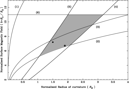
Figure 1: Plot of the normalized surface magnetic field $b=B_{s}/B_{d}$ versus normalized radius of curvature ${\cal R}_{6}={\cal R}/R$. Lines (1) to (6) in the above figure correspond to eqs. (1) to (6) in the text. The allowed parameter space for PSR B0943$+$10 is represented by the gray area. The two points with co-ordinates $({\cal R}_{6},b)$ marked by $\star$ and $\bullet$ represent two modelled cases (1.5, 7.2) and (1.9, 6.7), respectively, described in section 3 and presented in Figs. 2 and 3.

2.4 Parameter space

The surface magnetic field $B_{s}\sim B_{q}=4.4\times 10^{13}$ G represents the so-called photon splitting level, above which the electron-positron plasma cannot be produced (see Zhang & Harding 2000 for review). Hence, yet another constraint can be imposed for PSR B0943+10

$$b\leq\frac{B_{q}}{B_{d}}\sim 11.$$ (6)

Thus, the parameter space for possible values of $b$ and ${\cal R}_{6}$ is marked by the gray area enclosed by lines (6), (5), (4) and (2) in Fig. 1. Within this area the ICS-dominated NTVG can exist, with 20 equidistant sparks circulating around the perimeter of the polar cap in the time interval $\hat{P}_{3}$ close to 37 pulsar periods. The CR-NTVG represented by line (1) correspond to the case $k=0.5$ (for $k=1.0$ the limiting line $b=20\times{\cal R}_{6}^{0.31}$ almost coincides with the ordinate axis in Fig. 1; see also section 4). While we are not able to exclude the possibility of CR-NTVG formation, we find modelling of implied magnetic structure extremely difficult as we describe in section 3 and 4. As seen from Fig. 1, the surface magnetic field $B_{s}$ exceeds $2\times 10^{13}$ G $(b>3)$ and the radius of curvature ${\cal R}$ of surface field lines is about $(1-3)\times 10^{6}$ cm $(1\raisebox{-1.29167pt}{\mbox{$\stackrel{{\scriptstyle<}}{{{}_{\sim}}}\,$}}{\cal R}_{6}\raisebox{-1.29167pt}{\mbox{$\stackrel{{\scriptstyle<}}{{{}_{\sim}}}\,$}}3)$. The two filled symbols ($\star$ and $\bullet$) represent two model examples of the surface magnetic field structure which are discussed in the next section.

3 Modelling the surface magnetic field

We have argued that the observations of regularly drifting subpulses in PSR B0943+10 imply that ICS-dominated NTVG can form in this pulsar with a strong non-dipolar surface magnetic field. Further from Fig 1, we notice that the two parameters lie in the range $3\raisebox{-1.29167pt}{\mbox{$\stackrel{{\scriptstyle<}}{{{}_{\sim}}}\,$}}b\raisebox{-1.29167pt}{\mbox{$\stackrel{{\scriptstyle<}}{{{}_{\sim}}}\,$}}11$ and $0.33\raisebox{-1.29167pt}{\mbox{$\stackrel{{\scriptstyle<}}{{{}_{\sim}}}\,$}}\rho_{c}\raisebox{-1.29167pt}{\mbox{$\stackrel{{\scriptstyle<}}{{{}_{\sim}}}\,$}}1$, where we introduce the normalized curvature $\rho_{c}=1/{\cal R}_{6}$. We now examine by means of numerical modelling whether such a structure of the surface magnetic field is conceivable. We assume that the actual surface magnetic field is a superposition of the star centered global dipole moment ${\bf d}$ and the crust anchored dipole moment ${\bf m}$ placed at ${\bf R}_{m}$, whose influence results in small scale deviations of the surface field from the pure global dipole. The resultant surface magnetic field ${\bf B}_{s}={\bf B}_{d}+{\bf B}_{m}$, where $|{\bf B}_{d}|\sim 2d/r^{3}$ and $|{\bf B}_{m}|\sim 2m/|{\bf r}-{\bf R}_{m}|^{3}$, where ${\bf r}$ is the radius vector. For clarity of graphic presentation we use the normalization $R_{0}=|{\bf R}_{m}|/R$ and the strength of $m=|{\bf m}|$ is expressed in units of $d=|{\bf d}|$.

The detailed numerical formalism of modelling the actual surface magnetic field within the above model was developed by Gil et al. (2002) and we now apply it to PSR B0943+10. This accompanying paper gives details of modelling of the surface magnetic field in pulsars (a review concerning the crust origin surface magnetic field in pulsars is also included in this paper). To obtain the equations of resultant open magnetic field lines (along which a high unipolar potential drop can develop) we solve the system of differential equations $d\theta/dr=B_{\theta}/(rB_{r})$ and $d\phi/dr=B_{\theta}(rB_{r}\sin\theta)$, with the initial condition $B_{m}(r=5R)=0$ (since $B_{m}/B_{d}\sim(m/d)(r/|{\bf r}-{\bf R}_{m}|)^{3}$, then for $m/d\sim 10^{-4}$ the ratio $B_{m}/B_{d}\sim 10^{-4}$ for $r\raisebox{-1.29167pt}{\mbox{$\stackrel{{\scriptstyle>}}{{{}_{\sim}}}\,$}}5R$). Thus, we define a bundle of the open dipolar field lines at the altitude $r=5R$ and then trace the lines of resultant magnetic field ${\bf B}_{s}$ down to the stellar surface $(r=R)$. Consequently, we obtain the boundary of the physical polar cap as well as the actual surface magnetic field above the polar cap. It follows from the symmetry suggested by the observed patterns of drifting subpulses and their spectral analysis (DR99, DR01) that the local dipole ${\bf m}$ should lie in the fiducial plane containing both the pulsar spin axis and the magnetic axis. Without loss of generality, we placed for simplicity the local dipole axis at the polar cap center. Since $B_{s}\gg B_{d}$ in PSR B0943$+$10 then in order to increase $B_{d}$ to values exceeding $10^{13}$ G the magnetic moments ${\bf d}$ and ${\bf m}$ must have the same polarity.

Figure 2: Structure of the surface magnetic field ${\bf B}_{s}$ for a superposition of the global star centered dipolar moment and crust anchored dipole moment described by: $m=2.85\times 10^{-4}\leavevmode\nobreak\ d$ and $R_{0}=0.967\leavevmode\nobreak\ R$ ($\star$) and $m=1.73\times 10^{-4}\leavevmode\nobreak\ d$ and $R_{0}=0.975\leavevmode\nobreak\ R$ ($\bullet$), respectively. The horizontal axis is labelled by the azimuthal angle $\theta$ (magnetic co-latitude). The vertical axis is labelled by the normalized surface magnetic field $b=B_{s}/B_{d}$ in the upper panel, and by the normalized altitude $z=r/R$ in the lower panel. The angular size of the canonical ($\theta_{d}$–dipolar) and the actual ($\theta_{s}$–non-dipolar) polar cap is marked by dotted and dashed vertical lines, respectively. The converging magnetic field lines presented in the lower panel correspond to both cases, but, given the proximity of the two structures, cannot be distinguished within the graphic resolution.

Fig. 2 presents results of calculations for two cases: $m=2.1\times 10^{-4}d$ and $R_{0}=0.967R$ (marked as $\star$), and $m=1.0\times 10^{-4}d$ and $R_{0}=0.975R$ (marked as $\bullet$). The lower panel presents the actual surface magnetic fields (as a function of normalized altitude $z=r/R$) for both cases, however, the proximity of the structures makes it difficult to distinguish them in the plotted scale. The abscissa is labelled by the azimuthal angle $\theta$ (magnetic colatitude), which measures the polar cap radius in radians. For a purely dipolar magnetic field $r_{p}=R\cdot\sin\theta_{d}\approx 10^{4}P^{-1/2}$ cm, which corresponds to $|\theta_{d}|\sim 0.01$ radians (marked by two vertical dotted lines). The actual polar cap is much narrower, with $|\theta_{s}|\sim 0.004$ radians (marked by two vertical dashed lines) or $r_{s}\sim 0.4r_{d}$. Near the last open magnetic field lines (thick lines in the lower panel) $b=6.7$ ($\bullet$) and $b=7.2$ ($\star$), respectively.

Fig. 3 shows the average normalized curvature $\rho_{c}=1/{\cal R}_{c}$ of the two outermost (thick) magnetic field lines shown in Fig. 2. The horizontal axis is labelled by $\zeta=z-1$, where $z=r/R$ (Fig. 2). The dashed vertical line corresponds to the characteristic gap height $h\approx 500$ cm. As follows from the parameter space marked by the gray area in Fig. 1, the normalized radius of curvature $1\raisebox{-1.29167pt}{\mbox{$\stackrel{{\scriptstyle<}}{{{}_{\sim}}}\,$}}{\cal R}_{6}\raisebox{-1.29167pt}{\mbox{$\stackrel{{\scriptstyle<}}{{{}_{\sim}}}\,$}}3$ and thus the normalized curvature $0.33\raisebox{-1.29167pt}{\mbox{$\stackrel{{\scriptstyle<}}{{{}_{\sim}}}\,$}}\rho_{c}\raisebox{-1.29167pt}{\mbox{$\stackrel{{\scriptstyle<}}{{{}_{\sim}}}\,$}}1$. Therefore, conditions for the formation of the ICS-NTVG are satisfied within the gray area marked in Fig. 3. This corresponds to an annular region at the periphery of the polar cap (with size comparable with the gap height $h_{ICS}\sim 0.15r_{p})$, and can accommodate only one ring of 20 drifting sparks (with ${\cal D}\sim h_{ICS}$). Within the central region inside this ring, the polar gap with sparking discharges cannot develop. Thus, either the central part of the beam of PSR B0943$+$10 is radio-quiet (hollow-cone) or its radio emission is driven by the stationary free-flow (e.g. Sharleman et al. 1978) instead of nonstationary spark-associated flow (RS75).

As it can be seen from Fig. 3, the crust-origin magnetic field decays rapidly with altitude and at $\zeta>0.3$ ($z>1.3$) the normalized curvature $\rho_{c}\simeq 0.007$ (${\cal R}_{6}\simeq 150$), suggesting almost for purely dipolar field. Moreover, the sign of $\rho_{c}$ in the region of dipolar field lines is negative, while within the gap (and its vicinity) $\rho_{c}$ is positive. Thus, the geometry of the surface magnetic fields lines within the gap is converging, implying that the radius of curvature is directed towards the pole (opposite to the case of diverging dipolar field lines). Therefore, the magnetic field driven spark discharges will tend to occupy the peripheral areas of the polar cap, instead of moving rapidly towards the pole (Cheng & Ruderman, 1977; Filippenko & Radhakrishnan, 1982). This should have a stabilizing effect on the arrangement of 20 sparks circulating around the perimeter of the polar cap in PSR B0943$+$10.

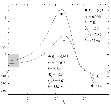
Figure 3: Plot of the normalized curvature $\rho_{c}$ averaged for the outermost open magnetic field lines (thick lines in Fig. 2) versus the normalized altitude expressed in the form $\zeta=z-1$, where $z=r/R$ (Figs. 2 and 3). The parameters of the modelled points marked by $\star$ and $\bullet$ are given. The gray area indicates values of $\rho_{c}$ for which the ICS-NTVG can form in PSR B0943$+$10. The vertical dashed line represents the VG height $h\sim 500$ cm.

4 Summary

In this paper we explored consequences of the vacuum gap model interpretation of drifting subpulses in PSR B0943$+$10, where 20 sparks move circumferentially around the perimeter of the polar cap, each completing one circulation in 37 pulsar periods (DR99, DR01). Both the characteristic spark dimension $\mathcal{D}$ and mutual distance $d$ between adjacent sparks are assumed to be about the polar gap height $h$. The formation of the vacuum gap requires extremely strong non-dipolar surface magnetic (GM01). We considered both the CR and resonant ICS seed photons as sources of electron-positron pairs and determined the parameter space for the surface magnetic field structure in each case. For the CR-NTVG ($k=0.5$) the surface magnetic field strength $B_{s}>2\times 10^{13}$ G and the radius of curvature of surface field lines $6\times 10^{4}\mathrm{cm}<\mathcal{R}<12\times 10^{4}\mathrm{cm}$, while for the resonant ICS-NTVG $B_{s}>2\times 10^{13}$ G and $10^{6}\mathrm{cm}<\mathcal{R}<3\times 10^{6}\mathrm{cm}$ (in both cases $B_{s}<B_{q}\sim 4.4\times 10^{13}$ G). Our modelling favours ICS-NTVG formation (refer Fig. 1) although CR-NTVG cannot be excluded. The ICS photon driven vacuum gap supported by the magnetic field structure determined by this parameter space guarantees a system of 20 sparks with $\mathcal{D}\sim d\sim h_{ICS}$, circulating around the perimeter of the polar cap by means of the $\mathbf{E}\times\mathbf{B}$ drift in about 37 pulsar periods. This phenomenon is most probably observed in the form of drifting subpulses in PSR B0943$+$10.

We modelled the magnetic field structure using a simple and quite general model in which the actual surface magnetic field at the polar cap is a superposition of global core-anchored dipole $\mathbf{B}_{d}$ (inferred from pulsar spin down) and local crust-anchored dipole $\mathbf{B}_{m}$ (Gil et al., 2002). Since $B_{d}=6.4\times 10^{12}(P\cdot\dot{P})^{1/2}\mathrm{G}=4\times 10^{12}$ G, then in order to obtain $\mathbf{B}_{s}\sim(2\div 3)\times 10^{13}$ G one needs to assume $B_{m}\gg B_{d}$ and the same polarity of both components. Following the symmetry suggested by observed patterns of drifting subpulses in PSR B0943$+$10, we placed the local dipole axis at the polar cap center. Two examples of model solutions $(b,\mathcal{R})$ are shown in Fig. 1 marked as $\star$ and $\bullet$ within the gray area. More details concerning these two solutions are presented in Figs. 2 and 3. Our modelling yields a number of important conclusions: (i) The conditions for the formation of the ICS-NTVG are satisfied only at peripheral ring-like region of the polar cap which can just accommodate a system of 20 $\mathbf{E}\times\mathbf{B}$ drifting sparks with $\mathcal{D}\sim d\sim h_{ICS}$. (ii) The surface magnetic field lines within the actual gap are converging, which stabilizes the $\mathbf{E}\times\mathbf{B}$ drifting sparks by preventing them from rushing towards the pole (as in the case of diverging dipolar field). (iii) No model solutions could be obtained close to or above the line (3) in Fig. 1 (especially for $\mathcal{R}_{6}>1.5$), corresponding to the efficiency parameter² $k=1$. This means that $k\raisebox{-1.29167pt}{\mbox{$\stackrel{{\scriptstyle<}}{{{}_{\sim}}}\,$}}0.8$ ($\bullet$ in Fig. 1), at least in PSR B0943$+$10. (iv) We find no model solutions in the range $b\sim$ 7 to 10 and $\mathcal{R}_{6}\sim$ 0.06 to 0.12, corresponding to the CR-NTVG parameter space (not shown in Fig. 1). This favors the ICS-NTVG in PSR B0943$+$10. We emphasize that conclusions (ii)-(iv) result from a specific dependence of $b$ on ${\cal R}_{b}$ following from central position of the local surface dipole ${\bf B}_{m}$, which seems to be justified in this case by apparent symmetries inferred from the observational data of PSR B0943$+$10.

The sparks inherent to the vacuum gap model not only provide a natural explanation for drifting subpulses but they also imply a mechanism of their radio emission. Melikidze et al. (2000) proposed a spark-associated model for coherent pulsar radio emission by means of curvature radiation of charged relativistic solitons and we will apply this model to the ICS-NTVG in PSR B0943$+$10 in the forthcoming paper.