Global m=1 modes and migration of protoplanetary cores in eccentric protoplanetary discs

Abstract

We calculate global $m=1$ modes with low pattern speed corresponding to introducing a finite eccentricity into a protoplanetary disc. We consider disc models which are either isolated or contain one or two protoplanets orbiting in an inner cavity. Global modes that are strongly coupled to inner protoplanets are found to have disc orbits which tend to have apsidal lines antialigned with respect to those of the inner protoplanets. Other modes corresponding to free disc modes may be global over a large range of length scales and accordingly be long lived. We consider the motion of a protoplanet in the earth mass range embedded in an eccentric disc and determine the equilibrium orbits which maintain fixed apsidal alignment with respect to the disc gas orbits. Equilibrium eccentricities are found to be comparable or possibly exceed the disc eccentricity. We then approximately calculate the tidal interaction with the disc in order to estimate the orbital migration rate. Results are found to deviate from the case of axisymmetric disc with near circular protoplanet orbit once eccentricities of protoplanet and disc orbits become comparable to the disc aspect ratio in magnitude. Aligned protoplanet orbits with very similar eccentricity to that of the gas disc are found to undergo litle eccentricity change while undergoing inward migration in general. However, for significantly larger orbital eccentricities, migration may be significantly reduced or even reverse from inwards to outwards. Thus the existence of global non circular motions in discs with radial excursions comparable to the semi-thickness may have important consequences for the migration and survival of protoplanetary cores in the earth mass range.

iant planet formation - extrasolar planets - - orbital migration - resonance-protoplanetary discs - stars: individual: Ups And

1 Introduction

The recent discovery of a number of extrasolar giant planets orbiting around nearby solar–type stars ( Mayor & Queloz, 1995, Marcy & Butler 1998, 2000) reveals that they have masses that are comparable to that of Jupiter, have orbital semi-major axes in the range

$0.04\;{\rm AU}\;\;\raisebox{-3.44444pt}{$\buildrel\textstyle<\over{\sim}$}\;\;a\;\;\raisebox{-3.44444pt}{$\buildrel\textstyle<\over{\sim}$}\;\;2.5\;{\rm au}$, and orbital eccentricities in the range $0.0\;\;\raisebox{-3.44444pt}{$\buildrel\textstyle<\over{\sim}$}\;\;e\;\;\raisebox{-3.44444pt}{$\buildrel\textstyle<\over{\sim}$}\;\;0.93.$

Orbital migration originally considered as a mechanism operating in protoplanetary discs by Goldreich & Tremaine (1980) has been suggested as an explanation for the existence of giant planets close to their central star (eg. Lin, Bodenheimer, & Richardson 1996). Protoplanetary cores are thought to form at several astronomical units and then migrate inwards either before accumulating a gaseous envelope and while in the earth mass range (type I migration) or in the form of a giant planet (type II migration) (see for example Lin & Papaloizou 1993, Ward 1997). In the former case the interaction with the disc is treated in a linearized approximation ( eg. Goldreich & Tremaine 1980) while in the latter nonlinearity is important leading to gap formation ( eg. Bryden et al 1999, Kley 1999). Both types of migration heve been found to occur on a timescale more than one order of magnitude shorter than that required to form giant planets or the expected lifetime of the disc and accordingly the survival of embryo protoplanets is in question ( eg. Ward 1997, Nelson et al 2000 ). Accordingly mechanisms that slow or halt migration such as the entry into a magnetospheric cavity close to the star ( Lin, Bodenheimer, & Richardson 1996) have been suggested. However, the existence of giant planets over a range of semi-major axes suggests that a more general mechanism for halting migration should be sought.

In this paper we shall consider effects produced when the large scale motion of the disc gas deviates from that of pure circular motion about the central mass as could be produced when the disc becomes eccentric as happens when it supports a global $m=1$ mode. Such modes could be produced by disc protoplanet interactions (eg. Papaloizou, Nelson & Masset 2001). However, for standard parameters, it was found that an instability leading to an eccentric disc together with an eccentric protoplanet orbit occurred only for large masses exceeding about fifteen Jupiter masses.

In this context note these calculations were done for laminar model discs with anomalously large viscosity coefficient and results may be somewhat different for turbulent discs. These simulations as well as resonant torque calculations appropriate to embedded cores by Papaloizou & Larwood (2000) have indicated possible reversal of orbital migration associated with eccentric orbits with modest eccentricity comparable to the disc aspect ratio.

This leads us to study further the dynamics of protoplanetary cores, massive enough for tidal interactions with the disc to be more important than effects due to gas drag, in an eccentric protoplanetary disc. In this paper we consider large scale $m=1$ modes in gaseous protoplanetary discs that correspond to making them eccentric. These modes have a low frequency branch for which the disc gas follows trajectories differing from Keplerian eccentric orbits by small corrections depending on forces due to disc self-gravity and pressure. These modes can be global in that they may vary on a length scale comparable to that of the whole disc even though it might have a large dynamic range. We shall consider a ratio of outer to inner radius of one hundred. These modes are of interest because, even though no definitive excitation mechanism of general applicability has yet been identified, their large scale implies a long life time comparable to the viscous time of the disc making them of potential interest in Astrophysics ( eg. Ogilvie 2001). They have also been considered as a potential source of angular momentum transport by Lee & Goodman (1999) in a tight winding approximation. Furthermore a disc composed of many stars on near Keplerian orbits has been postulated to occur in such objects as the nucleus of M31 (Tremaine 1995).

Here we consider global $m=1$ modes for various disc models neglecting viscous processes which are presumed to act over a longer time scale than that appropriate to the phenomena of interest. For global disturbances in protoplanetary discs of the type we consider, inclusion of self-gravity is important. Even though the discs are gravitationally stable, pressure and self-gravity can be equally important on scales comparable to the current radius, $r,$ when the Toomre stability parameter $Q\sim r/H,$ with $H$ being the disc semi-thickness. This condition is satisfied for typical protostellar disc models ( eg. Papaloizou & Terquem 1999). In addition to this, disc self-gravity has to be considered in the description of the motion of embedded protoplanets and it generally causes them to move in eccentric orbits, with eccentricity comparable to or exceeding that in the disc. We find that circularization due to tidal interaction with the disc may play only a minor role if the local test particle precession frequency relative to the disc is large compared to the circularization rate. We also find that for modest disc eccentricities comparable to the aspect ratio $H/r,$ disc tidal interactions may differ significantly from those found in axisymmetric discs. This in turn may have important consequences for estimates of orbital migration rates for protoplanetary cores in the earth mass range.

In section 2 we give the Basic equations and the linearized form we use to calculate global $m=1$ modes with low pattern speed corresponding to introducing a finite disc eccentricity. We go on to describe the disc models used which may contain protoplanets orbiting in an inner cavity. In section 3) we present the results of normal mode calculations. We go on to discuss the motion of a protoplanet in the earth mass range in an eccentric disc in section 4, determining the equilibrium (non precessing) orbits which maintain apsidal alignment with the disc gas orbits. We then formulate the calculation of the tidal response of an eccentric disc to a low mass protoplanet in section 5 determining the time rate of change of the eccentricity and orbital migration rate. We find that aligned orbits with very similar eccentricity to that of the gas disc may suffer no eccentricity change while undergoing inward migration in general. However, when the non precessing aligned orbit has a significantly higher eccentricity than the disc, as can occur for modes with very small pattern speed, orbital migration may be significantly reduced or reverse from inwards to outwards for the disc models we consider. This finding is supported by a local dynamical friction calculation applicable when the protoplanet eccentricity is much larger than the disc aspect ratio. Finally we go on to discuss our results in section 7.

2 Basic equations and their linearized form for large scale global modes with $m=1.$

We work in a non rotating cylindrical coordinate system $(r,\varphi)$ which may initially be considered to be centred on the primary star. The basic equations of motion in a two dimensional approximation which should be appropriate for a large scale description of the disc are taken to be

$${\partial v_{r}\over\partial t}+v_{r}{\partial v_{r}\over\partial r}+{v_{\varphi}\over r}{\partial v_{r}\over\partial\varphi}-{v_{\varphi}^{2}\over r}=-{1\over\Sigma}{\partial\Pi\over\partial r}-{\partial\Phi\over\partial r},$$ (1)

$${\partial v_{\varphi}\over\partial t}+v_{r}{\partial v_{\varphi}\over\partial r}+{v_{\varphi}\over r}{\partial v_{\varphi}\over\partial\varphi}+{v_{\varphi}v_{r}\over r}=-{1\over r\Sigma}{\partial\Pi\over\partial\varphi}-{1\over r}{\partial\Phi\over\partial\varphi},$$ (2)

In addition we have the two dimensional form of the continuity equation

$${\partial(r\Sigma)\over\partial t}+{\partial\left(r\Sigma v_{r}\right)\over\partial r}+{\partial\left(r\Sigma v_{\varphi}\right)\over\partial\varphi}=0.$$ (3)

Here the velocity is ${\bf v}=(v_{r},v_{\varphi}),$ $\Pi=\int^{\infty}_{-\infty}Pdz$ represents a vertically integrated pressure which we assume to be a function of the surface density $\Sigma$ defined by

$$\Sigma=\int^{\infty}_{-\infty}\rho dz.$$ (4)

The sound speed is then given by $c=\sqrt{d\Pi/d\Sigma}.$ The gravitational potential $\Phi=-GM_{*}/r+\Phi_{D}+\Phi_{ext},$ with $G$ being the gravitational constant, has a point mass contribution arising from the central mass $M_{*},$ a contribution, $\Phi_{D},$ due to the disc and a contribution, $\Phi_{ext},$ due to external protoplanets.

The unperturbed disk is axisymmetric with no radial motion such that the velocity ${\bf v}=(0,r\Omega)$ with $\Omega>0.$ In equilibrium we then have from equation (1)

$${\Omega^{2}r}={1\over\Sigma}{\partial\Pi\over\partial r}+{\partial\Phi\over\partial r}$$ (5)

and the gravitational potential due to the disc is given by

$$\Phi_{D}=-G\int\Sigma K(r,r^{\prime})r^{\prime}dr^{\prime},$$ (6)

with

$$K_{0}(r,r^{\prime})=\int^{2\pi}_{0}{1\over\sqrt{(r^{2}+r^{\prime 2}-2rr^{\prime}\cos(\varphi))}}d\varphi.$$ (7)

We allow for the effects of orbiting external protoplanets which provide the external potential $\Phi_{ext}.$ In this paper we are primarily interested in phenomena which vary on a time scale long compared to a local orbital period. Accordingly we use the time averaged or secular protoplanet perturbing potential which is derived in Appendix 1. For a single protoplanet of mass $m_{p}$ and orbital radius $r_{p},$ the contribution to the external potential is given by

$$\Phi_{ext}=-G{m_{p}\over 2\pi}K_{0}(r,r_{p}).$$ (8)

In a thin disc of the kind considered here, the contributions due to pressure and self-gravity are comparable and small leading to nearly Keplerian rotation which has $\Omega\propto r^{-3/2}.$ When $c\propto r^{-1/2},$ the disc then has a nearly constant putative aspect ratio $H/r=c/(r\Omega),$ $H$ being the putative semi thickness.

2.1 Linearization

Here we are interested in global $m=1$ modes with slowly varying pattern when viewed in the adopted reference frame. To study these, we linearize the basic equations about the equilibrium state denoting perturbations to quantities with a prime.

As usual we assume that the dependence of all perturbations (in cylindrical coordinates) on $\varphi$ and $t$ is through a factor $\exp i\left(m\left(\varphi-\Omega_{p}t\right)\right).$ For the slowly varying modes we consider $\Omega_{p}<<\Omega.$

The linearized forms of equations (1) ,(2) and (3) are then

$$im(\Omega-\Omega_{p})v^{\prime}_{r}-2\Omega v^{\prime}_{\varphi}=-{\partial W\over\partial r},$$ (9)

$$im(\Omega-\Omega_{p})v^{\prime}_{\varphi}+{\kappa^{2}\over 2\Omega}v^{\prime}_{r}=-{imW\over r},$$ (10)

and

$${im(\Omega-\Omega_{p})\Sigma(W-\phi^{\prime})\over c^{2}}=-{1\over r}{\partial\left(r\Sigma v^{\prime}_{r}\right)\over\partial r}-{im\Sigma v^{\prime}_{\varphi}\over r}.$$ (11)

Here $W=\Pi^{\prime}/\Sigma+\Phi^{\prime}=\Sigma^{\prime}c^{2}/\Sigma+\Phi^{\prime},$

and $\kappa^{2}=(2\Omega/r)(d(r^{2}\Omega)/dr)$ denotes the square of the epicyclic frequency.

For the gravitational potential perturbation we have $\Phi^{\prime}=\Phi_{D}^{\prime}+\Phi^{\prime}_{ext}.$ Here we shall allow for the contribution of the secular effects of other sources such as protoplanets to the modes through the gravitational potential perturbation $\Phi^{\prime}_{ext}.$

2.2 Slowly varying modes with m=1

We consider linear perturbations of an axisymmetric disc that correspond to normal modes with $m=1$ that make it eccentric. The modes we consider are such that $\Omega_{p}<<\Omega$ and the dominant motion is epicyclic. In this case, to lowest order, we may neglect the pressure and self-gravity term $W$ as well as $\Omega_{p}$ and assume $\Omega$ is keplerian, to obtain from equation (10)

$$iv^{\prime}_{\varphi}=-{1\over 2}v^{\prime}_{r}.$$ (12)

Using the above and introducing the radial Lagrangian displacement $\xi_{r}=-iv^{\prime}_{r}/(\Omega-\Omega_{p}),$ equation (11) gives the surface density perturbation in the low frequency limit in the form

$$\Sigma^{\prime}=-r{d(\Sigma e(r))\over dr},$$ (13)

with $e(r)\equiv\xi_{r}/r$ being the disc eccentricity.

The gravitational potential perturbation induced by the disc is

$$\Phi^{\prime}_{D}=-G\int\Sigma^{\prime}K_{1}(r,r^{\prime})r^{\prime}dr^{\prime},$$ (14)

with

$$K_{1}(r,r^{\prime})=\int^{2\pi}_{0}{\cos(\varphi)\over\sqrt{(r^{2}+r^{\prime 2}-2rr^{\prime}\cos(\varphi))}}d\varphi-{\pi r\over r^{\prime 2}},$$ (15)

where the second term corresponds to the indirect term which results from the acceleration of the coordinate system produced by the disc material.

The existence of a mode with $m=1$ in the disc causes the orbits of the protoplanets interior to the disc to become eccentric. Noting the different form of indirect term used, the secular perturbing potential derived in Appendix 1 then gives the contribution of an orbiting protoplanet to the external potential perturbation to be

$$\Phi^{\prime}_{p}(r)=-{Gm_{p}\xi_{r}(r_{p})\over 2\pi r_{p}^{2}}{\partial\over\partial r_{p}}\left(K_{1}(r,r_{p})r_{p}^{2}\right).$$ (16)

Here the eccentricity of the companion orbit is related to the displacement by $e_{p}=\xi_{r}(r_{p})/r_{p}.$ The total external potential perturbation is then found by summing over the perturbing protoplanets:

$$\Phi^{\prime}_{ext}(r)=\sum_{p}\Phi^{\prime}_{p}(r)$$ (17)

Eliminating $v_{\varphi}^{\prime}$ from equations (9) and (10), using equation (13) for $\Sigma^{\prime}$ and expanding to first order in the small frequencies $\Omega_{p}$ and $\omega_{p}=\Omega-\kappa,$ the fluid element orbital precession frequency in the absence of surface density or gravitational potential perturbations, one obtains a normal mode equation relating $e(r),e_{p}$ and $\Omega_{p}$ in the form (see also Papaloizou, Nelson & Masset, 2001)

$$2\left(\Omega_{p}-\omega_{p}\right)\Omega r^{3}e(r)={d\over dr}\left({r^{3}c^{2}\over\Sigma}{d[\Sigma e(r)]\over dr}\right)-{d\left(r^{2}\Phi^{\prime}\right)\over dr},$$ (18)

where $,c,$ is the local sound speed.

In addition we have an equation for each protoplanet of the form

$$2\left(\Omega_{p}-\omega_{p}\right)\Omega(r_{p})r_{p}^{3}e_{p}=-\left[{d\left(r^{2}\Phi^{\prime}\right)\over dr}\right]_{r=r_{p}},$$ (19)

where of course for a particular protoplanet there is no self-interaction term in the sum for $\Phi^{\prime}_{ext}.$ The inclusion of self-gravity in the eigenvalue problem is essential if modes with prograde precession frequency are to be obtained. For typical protoplanetary disc models, self-gravity can be strong enough to induce prograde precession for the long wavelength $m=1$ modes considered here.

Normal modes were calculated by discretizing (18) and (19) and formulating a matrix eigenvalue problem on an unequally spaced grid with $200$ grid points with intervals increasing in geometric progression (see Terquem & Papaloizou 2000 for consideration of a related problem).

2.3 Disc models

We present here results obtained for a disc model with equation of state given by a polytrope of index $n=1.5.$ The sound speed is given by

$$c^{2}={GM_{*}H^{2}\over R_{in}^{3}}\left(1-\left(R_{in}/r\right)^{10}\right)\left(1-\left(r/R_{out}\right)^{10}\right)R_{in}/r.$$ (20)

Here the first two factors provide sharp edges at the disc inner and outer boundaries and $H/r=0.05$ is the disc aspect ratio away from these boundaries.

The surface density is given by

$$\Sigma=\Sigma_{0}(c^{2})^{n}.$$ (21)

The boundary regions are chosen to be of order the disc scale height in width and away from these $\Sigma\propto r^{-3/2}.$ In the above $R_{in}$ is the inner boundary radius which is taken to be the unit of length. The unit of mass is the central mass $M_{*}$ and the unit of time is $R_{in}^{3/2}/\sqrt{GM_{*}}.$ The arbitrary scaling factor $\Sigma_{0}$ was chosen such that in model $A$ the total disc mass was $4.0\times 10^{-2}M_{*}.$ In model $B$ the total disc mass was $4.0\times 10^{-3}.$ $R_{out}$ is the outer boundary radius, here, in order to study large scale modes, taken as $100R_{in}.$

The importance of self gravity is measured by the Toomre parameter $Q=\Omega c/(\pi G\Sigma).$ For model A this has a minimum value of $5.2$ while for the lower mass disc model of model B this minimum value is $52.$ Another quantity of interest is the local precession frequency of a test particle orbit $\omega_{pg}$ in the axisymmetric component of the total gravitational potential ( see equation (29) below).

Figure 1: This figure shows the local test particle orbital precession frequency in dimensionless units as a function of radius, $r$ in units of $R_{in}$ in the range $1.1<r<100$ for the two disc models A (lower curve) and B with no interior orbiting protoplanets. Apart from small regions near to the boundaries, the frequency is negative corresponding to retrograde precession.

This is plotted for the two disc models in figure 1. It is small and negative in dimensionless units over much of the discs, corresponding to retrograde precession, scaling with the disc mass as it is determined by the disc self-gravity. As we shall see this behaviour provides scope for secular resonance associated with low frequency modes.

3 Normal modes

We have calculated the lowest order global normal modes for two different configurations involving protoplanets orbiting interior to the disc in an inner cavity. The first, approximating the Upsilon Andromedae system involves two protoplanets with mass ratios $0.00383$ and $0.00196$ orbiting at $0.6R_{in}$ and $0.194R_{in}$ respectively. However, the disc normal modes do not change much in character if the protoplanet orbital radii are scaled to somewhat smaller fractions of $R_{in}.$ But the ratio of protoplanet to disc eccentricity in the joint modes changes more significantly. The second configuration we consider is a single protoplanet with mass ratio $0.002$ orbiting at $0.6R_{in}.$ Finally we consider a disc with no interior orbiting protoplanets. In all of these cases we consider both model $A$ and model $B$ discs.

The pattern speeds for the highest frequency normal modes and the protoplanet orbital eccentricities occurring jointly with the normal modes are given in table 1. For the results presented here, the modes are normalized such that the disc eccentricity at the inner boundary is 0.1.

Figure 2: This figure shows the first two modes and the associated equilibrium eccentricities as a function of radius $r$ in units of $R_{in}$ for the two protoplanet case with disc model A. The two modes (full curves) are normalized so that $e=0.1$ at $r=1.$ The lower curve corresponds to the mode of highest frequency given in table 1. The dotted curves give the associated equilibrium eccentricities calculated for a low mass protoplanet orbiting within the disc, the lowermost corresponding to the highest frequency mode. The dashed curve gives the equilibrium eccentricity for a low mass protoplanet orbiting within the disc calculated for the highest frequency mode but neglecting the non axisymmetric component of the disc potential. The dot dashed curve gives the corresponding plot for the other mode. The latter curves indicate the presence of secular resonances at $r\sim 1.1$ associated with both modes.

Figure 3: As in figure 2 but for disc model B. In this case there is a secular resonance asociated with the highest frequency mode at $r\sim 1.1$. For the other mode this occurs at $r\sim 1.4.$

Many of the properties of these modes can be understood with reference to the local dispersion relation for density waves in the low frequency limit (Lin & Shu 1969) in the form

$$2\Omega(\omega_{p}-\Omega_{p})=-2\pi G\Sigma|k|+c^{2}k^{2},$$ (22)

where $k$ is the radial wavenumber. The above indicates that when self-gravity, governed by the first term on the right hand side, is unimportant as occurs for either low mass discs or large $|k|,$ $\Omega_{p}$ is negative. On the other hand positive $\Omega_{p}$ can occur for low $|k|$ or massive discs. Thus in that case the lowest order modes (in terms of numbers of nodes) should be prograde with more of these existing for more massive discs, a trend we find in our results. There can also be very low frequency (in magnitude) modes for which the self-gravity and pressure terms approximately cancel. This occurs when $|k|=2\pi G\Sigma/c^{2}\sim 2/(QH).$ For $Q\sim r/H$ as in the models here, this is comparable to the radius making a very global mode.

As we calculate normal modes jointly involving protoplanets and disc, the protoplanets have associated eccentricities. In general the ${\cal N}$ highest frequency modes predominantly involve the protoplanets while the others predominantly involve the disc, ${\cal N}$ being the number of protoplanets. The two highest frequency modes for the two protoplanet case are plotted in figure 2 for disc model $A$ and in figure 3 for disc model $B.$ For the second highest frequency mode calculated for disc model $A$, the protoplanet eccentricity ratio is $1.38,$ while for model $B$ it is $1.88.$ The latter result is similar to that given by Chiang, Tabachnik, & Tremaine (2001) who considered the current Upsilon Andromedae system with no disc and concluded it was predominantly in this mode.

Figure 4: This figure shows the four highest frequency modes as a function of radius $r$ in units of $R_{in}$ for the one planet model with disc A. The eccentricities are all normalized so that $e=0.1$ at $r=1.$ The modes can be identified by noting that the number of nodes increases with decreasing eigenfrequency.

Figure 5: As in figure 4 but for the one planet model with disc model $B.$

The results found here suggest the disc and protoplanet orbits were antialigned. With the outermost protoplanet at $0.6R_{in}$ the disc inner boundary and outer protoplanet eccentricities are comparable for model $A$ while for model $B$ the relative disc eccentricity is $56$ percent smaller. However, when the outer protoplanet orbits at $0.5R_{in}$ the disc inner boundary eccentricity is only $1/3$ that of the protoplanet for model $A$ and $19$ percent for model $B.$ Apart from the eccentricity scaling relative to the interior protoplanets, the spatial form of the eigenfunction in the disc remains almost identical.

Apart fom the two modes with highest frequency, other normal modes are essentially pure disc modes with only small associated protoplanet eccentricities.

Figure 6: As in figure 4 but for the disc model A with no protoplanets.

Figure 7: As in figure 6 but with disc model B

The four highest frequency modes for the one protoplanet case with disc model $A$ are plotted in figure 4 and in figure 5 for model $B.$ Pure disc modes with no protoplanet are plotted in figure 6 for model $A$ and figure 7 for model $B$. The modes develop increasing numbers of nodes as their frequency decreases but the mode with lowest frequency in absolute magnitude can be very global with only a few nodes out to $r=R_{out}.$ We comment that the modes are rather non compressive requiring eccentricities of order unity to provide Lagrangian changes in surface density of order unity. As the motion in the modes in linear theory is assumed epicyclic, this is suggestive that the analysis should be valid as long as the epicyclic approximation is.

Figure 8: This figure shows the form of the equilibrium eccentricity as a function of radius $r$ in units of $R_{in}$ for the modes shown in figure 4, the latter being normalized so that $e=0.1$ for $r=1.$ Curves are associated with normal modes according to increasing number of nodes. Thus the curve with the most nodes is associated with the normal mode with the most nodes. Note the secular resonances for $r<5.$

Figure 9: As in figure 8 but for the one planet model with disc model $B.$ Equilibrium curves are given for the two highest frequency modes only. That associated with the highest frequency decays to small values at about $r=5.$ The other curve shows a strong secular resonance at $r\sim 20.$

Having calculated these modes that may be largely driven by protoplanets in eccentric orbits or possibly self-excited or long lived structures we now go on to consider the migration of low mass protoplanets embedded in such eccentric discs.

Disc	$m_{p1}$	$m_{p2}$	$e_{p1}$	$e_{p2}$	$\Omega_{p}$
A	$.00383$	$.00196$	$-.36$	$1.82$	$1.61\times 10^{-3}$
A	$.00383$	$.00196$	$-.09$	$-.065$	$6.99\times 10^{-4}$
A	$.00383$	$.00196$	$.0068$	$.0029$	$3.01\times 10^{-5}$
A	$.00383$	$.00196$	$.0035$	$.0011$	$-5.10\times 10^{-4}$
B	$.00383$	$.00196$	$-.53$	$3.59$	$1.53\times 10^{-3}$
B	$.00383$	$.00196$	$-.18$	$-.094$	$3.58\times 10^{-4}$
B	$.00383$	$.00196$	$.0013$	$.00054$	$-6.53\times 10^{-6}$
B	$.00383$	$.00196$	$.0006$	$.0019$	$-4.40\times 10^{-4}$
A	$.002$	-	$-0.091$	-	$4.00\times 10^{-4}$
A	$.002$	-	$0.0136$	-	$4.02\times 10^{-6}$
A	$.002$	-	$0.0060$	-	$-4.06\times 10^{-4}$
A	$.002$	-	$0.0034$	-	$-9.17\times 10^{-4}$
B	$.002$	-	$-0.255$	-	$3.80\times 10^{-5}$
B	$.002$	-	$0.0122$	-	$6.62\times 10^{-6}$
B	$.002$	-	$0.0013$	-	$-3.55\times 10^{-4}$
B	$.002$	-	$0.0005$	-	$-9.70\times 10^{-4}$
A	-	-	-	-	$1.32\times 10^{-4}$
A	-	-	-	-	$3.26\times 10^{-6}$
A	-	-	-	-	$-1.58\times 10^{-4}$
A	-	-	-	-	$-4.12\times 10^{-4}$
B	-	-	-	-	$-6.15\times 10^{-5}$
B	-	-	-	-	$-1.60\times 10^{-4}$
B	-	-	-	-	$-3.74\times 10^{-4}$
B	-	-	-	-	$-5.77\times 10^{-4}$

Table 1: This table gives the protoplanet orbital eccentricities where appropriate together with the pattern speeds for the normal modes calculated. The disc model used is indicated in the first column, the protoplanet mass ratios to the central star in the second and third columns, their orbital eccentricities in the fourth and fifth column and the mode frequency or pattern speed in the sixth column. The modes are normalized such that the disc eccentricity at the inner boundary is 0.1. A negative protoplanet eccentricity then indicates the orbit is antialigned with the disc.

Figure 10: As in figure 8 but for the disc model $A$ with no protoplanets.

Figure 11: As in figure 10 but for the disc model $B$ with no protoplanets. In this case the longest wavelength equilibrium eccentricity indicates antialignment with the disc.

4 The motion of a low mass protoplanet in an eccentric disc

The evolution of the coplanar orbit of an interior protoplanet in the earth mass range embedded in the disc due to the gravitational interaction with the slowly precessing disc can be found using secular perturbation theory. We regard the embedded protoplanet as a test particle evolving in a prescribed gravitational potential and neglect the influence of the protoplanet on the disc mode. This should be reasonable when as here, the angular momentum of the protoplanet is significantly less than that of the material supporting the normal mode ( eg. Papaloizou et al 2001).

The orbit evolves under the perturbing potential per unit mass,

$${\cal{V}}\equiv\Phi_{D}+\Phi_{ext}=\Phi_{0}(r)+\Phi_{1}(r)\cos(\varphi-\Omega_{p}t).$$ (23)

Here $\Phi_{0}(r)$ is the axisymmetric component of the potential but excluding that due to the central mass and $\Phi_{1}(r)$ is the radial amplitude of the $m=1$ component arising from the normal mode.

On performing a time average over the protoplanet orbit one obtains the Hamiltonian system:

$${dh\over dt}=-{\partial{\cal{H}}\over\partial\alpha},\ \ \ \ {d\alpha\over dt}={\partial{\cal{H}}\over\partial h}.$$ (24)

Here $\alpha=\varpi-\Omega_{p}t,$ with $\varpi$ being the longtitude of periapse and ${\cal{H}}={\cal{V}}-\Omega_{p}h.$ The specific angular momentum is $h=\sqrt{GM_{*}a_{p}(1-e_{p}^{2})},$ $a_{p}$ is the constant semi-major axis, and $e_{p}$ is the eccentricity. To leading powers of $e_{p}$ we have

$${\cal{H}}=A(a_{p})+B(a_{p})e_{p}^{2}-\Omega_{p}h+C(a_{p})e_{p}^{4}+e_{p}D(a_{p})\cos\alpha.$$ (25)

Hamilton’s equations then give to leading powers of $e_{p}$

$${d\alpha\over dt}=-{2(B+e_{p}^{2}(2C-B/2))\over\sqrt{GM_{*}a_{p}}}-\Omega_{p}-{D(a_{p})\cos\alpha\over\sqrt{GM_{*}a_{p}}e_{p}}.$$ (26)

$${de_{p}\over dt}={\sqrt{1-e_{p}^{2}}\over\sqrt{GM_{*}a_{p}}e_{p}}{\partial{\cal{H}}\over\partial\alpha}=-{D(a_{p})\over\sqrt{GM_{*}a_{p}}}\sin\alpha.$$ (27)

Here the precession rate of the apsidal line induced by the axisymmetric potential, to first order in the perturbing potential, expressed as an expansion in powers of $e_{p}$ is given by the first term on the right hand of equation(26) as

$$\omega_{pg}=-{2\over\sqrt{GM_{*}a_{p}}}\left(B+e_{p}^{2}(2C-B/2)\right).$$ (28)

This may also be written in terms of the axisymmetric component of the potential directly as

$$2\omega_{pg}\sqrt{GM_{*}a_{p}^{5}}=(1+e_{p}^{2}){d^{2}\Phi_{0}\over du^{2}}+{e_{p}^{2}\over 8a_{p}^{2}}{d^{4}\Phi_{0}\over du^{4}},$$ (29)

where $u=1/r,$ and $r$ is taken to be equal to $a_{p}.$

Equilibrium or steady state solutions of (26) and (27) with $e_{p}$ and $\alpha$ constant occur when $\alpha=0$ or $\alpha=\pi.$ Adopting the convention that $e_{p}$ is positive suffices to select one of the latter possibilities as (26) gives an expression from which $e_{p}$ can be determined in the form

$$e_{p}=-{{D(a_{p})\cos\alpha}\over{{2(B+e_{p}^{2}(2C-B/2))}+\Omega_{p}\sqrt{GM_{*}a_{p}}}}.$$ (30)

or equivalently

$$e_{p}={{D(a_{p})\cos\alpha}\over{(\omega_{pg}-\Omega_{p})\sqrt{GM_{*}a_{p}}}}.$$ (31)

Alternatively one may fix $\alpha$ to be $0$ or $\pi$ and allow $e_{p}$ to change sign as we have done for the normal modes.

An equilibrium solution so determined corresponds to the situation when the protoplanet orbit precesses at the same rate, $\Omega_{p},$ as the mass distribution that produces the gravitational potential while maintaining a constant eccentricity. Assuming that $\omega_{pg}$ and $\Omega_{p}$ are of comparable magnitude, in general for modest eccentricity,

$$e_{p}\sim D(a_{p})/(\Omega_{p}\sqrt{GM_{*}a_{p}})\equiv e_{0}$$

and is proportional to the magnitude of the nonaxisymmetric potential. An exception occurs when

$${2B+\Omega_{p}\sqrt{GM_{*}a_{p}}}=0.$$

In this case, the precession frequency of a free orbit with small eccentricity, $\omega_{pg},$ matches that of the nonaxisymmetric mass distribution $\Omega_{p}$ corresponding to a secular resonance. When this occurs equation (30) indicates that $e_{p}\sim(e_{0})^{1/3}.$ Accordingly significantly larger equilibrium eccentricities are expected close to a secular resonance. We comment that for fixed $\alpha$ $e_{p}$ changes sign as a secular resonance is passed through corresponding to an alignment change through a rotation of the axis of the ellipse through $\pi.$

One may also investigate the effect of orbital circularization by adding a term $-e_{p}/|t_{e}|$ to the right hand side of (27), where $|t_{e}|$ is the circularization time. In this case one can still find an equilibrium but with orbital apsidal line rotated. Restricting consideration to the situation away from secular resonance, one finds that the equilibrium eccentricity is reduced by a factor $\sqrt{1+1/((\omega_{pg}-\Omega_{p})^{2}t_{e}^{2})}$ and $|\sin\alpha|=1/\sqrt{1+(\omega_{pg}-\Omega_{p})^{2}t_{e}^{2}}.$ Thus when $|(\omega_{pg}-\Omega_{p})t_{e}|$ is large, the effect of the circularization term is to produce a small rotation of the apsidal line of the orbit.

As indicated above equilibrium solutions correspond to the situation where the apsidal precession of the protoplanet orbit is locked to that of the underlying nonaxisymmetric disc.

One can find solutions undergoing small librations in the neighbourhood of equilibrium solutions (eg. Brouwer & Clemence 1961) and when dissipative forces are added these may decay making the attainment of equilibrium solutions natural. As we indicate below, tidal interaction of a protoplanet with the disc may produce such dissipative forces. Accordingly we shall focus on equilibrium solutions in what follows below.

4.1 Determination of equilibrium eccentricities corresponding to normal modes

It is a simple matter to determine equilibrium eccentricities for protoplanets moving under the gravitational potential appropriate to a normal mode corresponding to an eccentric disc, with pattern speed $\Omega_{p},$ of the type calculated above. We recall the normal mode equation(18) which can be regarded as determining the equilibrium disc eccentricity in the form

$$2\left(\Omega_{p}-\omega_{p}\right)\Omega r^{3}e(r)={d\over dr}\left({r^{3}c^{2}\over\Sigma}{d[\Sigma e(r)]\over dr}\right)-{d\left(r^{2}\Phi^{\prime}\right)\over dr}.$$ (32)

If the pressure forces are neglected by dropping the terms involving $c^{2},$ this is exactly equivalent to equation (31) for determining the protoplanet eccentricity with $e(r)$ corresponding to $e_{p}$ and $\omega_{p}$ replaced by $\omega_{pg}.$ Thus a local protoplanet equilibrium eccentricity appropriate to a disc mode or response can be determined by using the disc normal mode equation (18) retaining the term resulting from the disc self-gravity but omitting pressure contributions.

This procedure should be applicable provided the eccentricities are not too large. Equilibrium eccentricities are plotted for some of the normal modes we calculated in figures 2 and 3 and also 8 - 11. In figures 2 and 3 we also plot equilibrium eccentricities but calculated with the nonaxisymmetric contribution to the gravitational potential due to the disc removed which is equivalent to assuming that it remains circular. We see that the assumption that disc remains circular results in a significantly smaller equilibrium eccentricity for disc model A, particularly for the mode with second highest frequency. For the lower mass disc model B, differences arising fom assuming the disc remains circular are less pronounced. We also coment that the occurence of secular resonances in the inner parts of the disc where $r/R_{in}<10$ is common.

One expects that dissipative torques produced by

protoplanet-disc tidal interaction may result in the approach to such equilibrium solutions from general initial conditions. This we now discuss.

5 Response of an eccentric disc to a low mass protoplanet

To calculate the tidal response of an eccentric disc to a perturbing protoplanet it is convenient to introduce a new orthogonal coordinate system $(a,\lambda),$ with $a$ being the local semi-major axis and $\lambda$ being the orthogonal angular coordinate. Then taking pericentre in the disc to lie along $\varphi=0,$ $a=r(1+e\cos\varphi)/(1-e^{2}),$ with the eccentricity being a function of $a.$ We assume the eccentricity is small enough that we may work to first order in it and also that it has significant changes only on a global length scale comparable to $r.$ Then we may make the replacement $e(a)\equiv e(r).$ In this approximation $a$ can be expressed in terms of cylindrical coordinates in the form $a=r(1+e\cos\varphi)$ and the orthogonal angular coordinate, $\lambda$ is given by

$$\lambda=\varphi+\int({e\over r}dr)\sin\varphi,$$ (33)

where we may leave the integral as indefinite. It is also convenient to work in a frame in which the disc flow appears stationary. As the pattern speed as measured in an inertial frame is very small compared to the disc rotation speed, we shall neglect centrifugal and coriolis forces.

In a general orthogonal coordinate system in which the disc appears to be in a steady state, the equations of motion for the velocity $(v_{a},v_{\lambda})$ may then be written ( see Appendix 2)

$${\partial v_{a}\over\partial t}+v_{a}|\nabla a|^{2}{\partial\over\partial a}\left({v_{a}\over|\nabla a|}\right)+v_{\lambda}|\nabla a||\nabla\lambda|{\partial\left({v_{a}\over|\nabla a|}\right)\over\partial\lambda}$$

$$-{v_{\lambda}^{2}\over 2}|\nabla a||\nabla\lambda|^{2}{\partial\left(|\nabla\lambda|^{-2}\right)\over\partial a}-{v_{a}^{2}\over 2}|\nabla a|^{3}{\partial\left(|\nabla a|^{-2}\right)\over\partial a}$$

$$=-{|\nabla a|\over\Sigma}{\partial\Pi\over\partial a}-|\nabla a|{\partial\Phi\over\partial a},$$ (34)

$${\partial v_{\lambda}\over\partial t}+v_{\lambda}|\nabla\lambda|^{2}{\partial\left({v_{\lambda}\over|\nabla\lambda|}\right)\over\partial\lambda}+v_{a}|\nabla a||\nabla\lambda|{\partial\left({v_{\lambda}\over|\nabla\lambda|}\right)\over\partial a}$$

$$-{v_{a}^{2}\over 2}|\nabla a|^{2}|\nabla\lambda|{\partial\left(|\nabla a|^{-2}\right)\over\partial\lambda}-{v_{\lambda}^{2}\over 2}|\nabla\lambda|^{3}{\partial\left(|\nabla\lambda|^{-2}\right)\over\partial\lambda}$$

$$\ \ \ \ \ =-{|\nabla\lambda|\over\Sigma}{\partial\Pi\over\partial\lambda}-|\nabla\lambda|{\partial\Phi\over\partial\lambda},$$ (35)

We perform a response calculation by linearizing about a steady state in which the disc gas is taken to be in elliptical keplerian orbits with $v_{a}=0,$ and to first order in $e,$ $v_{\lambda}=(GM_{*}/a)^{1/2}(1+e\cos\lambda).$ In a thin disc forces due pressure and self-gravity provide only a small correction of order $(H/r)^{2}.$ We consider the situation when the disc eccentricity, $e(r),$ protoplanet eccentricity, $e_{p},$ and $H/r$ can be considered small and comparable in magnitude.

When considering the response to an embedded protoplanet, we are interested in responses with a scale $H$ and azimuthal mode number $m\sim r/H.$ Here for the time being $\lambda$ is regarded as the azimuthal angle. We perform a response calculation by linearizing equations (34) and (35) about the steady state described above. We may expand the linearized equations in powers of the disc eccentricity.

Here we shall work only to lowest order and neglect terms of order $e$ times smaller than the dominant ones which, linearizing (34) and (35) directly and denoting perturbation quantities by a prime, are of order $\Omega v_{a}^{\prime}.$ In this scheme we may replace $|\nabla a|$ and $|\nabla\lambda|$ by unity except where the latter occurs in the combination $|\nabla\lambda|v_{\lambda}{\partial\over\partial\lambda},$ with $|v_{\lambda}|$ here denoting the unperturbed velocity in the disc. This is because the contribution of terms of first order in the eccentricity to this operator leads to quantities of order $me|v_{\lambda}|v_{a}^{\prime}/r$ in the linearized equations. For $m\sim r/H,\sim 1/e$ these are comparable to the dominant terms. All other eccentricity contributions are smaller by a factor at most $\sim e.$

We have to first order in eccentricity

$$v_{\lambda}|\nabla\lambda|=(GM_{*}/a^{3})^{1/2}\left(1+2e\cos\varphi+\int({e\over r}dr)\cos\varphi\right).$$ (36)

Thus if we define a new angle $M$ through $M=\lambda-(2e+\int({e\over r}dr)\sin\lambda,$ the operator $|\nabla\lambda|v_{\lambda}{\partial\over\partial\lambda},$

becomes $=(GM_{*}/a^{3})^{1/2}{\partial\over\partial M}.$ The angle $M$ is just the mean anomaly as can be seen from the fact that to first order in $e,$

$$r=a(1-e\cos M),\varphi=M+2e\sin M,$$ (37)

For the motion of a particular disc particle we have $M=\Omega(t-t_{0}),$ where $t_{0}$ denotes the time of periastron passage.

To lowest order in $e,$ the coordinates $(a,M)$ behave just like the cylindrical coordinates $(r,\varphi)$ in the sense that one may make the replacements $r\rightarrow a,\varphi\rightarrow\lambda$ in the standard linearized equations expressed in cylindrical coordinates. However, recall that in the forcing potential $\Phi_{p}^{\prime},$ we must make the replacement (37) which can be thought of evaluation on an eccentric disc orbit.

5.1 Protoplanet forcing potential

Neglecting the indirect term, which does not contribute to the Fourier components with large $m\sim r/H$ of interest, the protoplanet forcing potential is

$$\Phi_{p}^{\prime}=-{Gm_{p}\over\sqrt{|r^{2}+R^{2}-2rR\cos(\varphi-\nu)+b^{2}|}}.$$ (38)

Here, the coordinates of the protoplanet are $(R,\nu)$ and $b$ is the softening parameter which is introduced to take account of the finite vertical thickness of the disc. In general $b\sim H$ ( eg. Artymowicz 1993).

For an eccentric protoplanet orbit with semi-major axis $a_{p}$ and eccentricity $e_{p},$ we have

$$R=a_{p}(1-e_{p}\cos(\omega t)),\nu=\omega t+\varpi+2e_{p}\sin(\omega t).$$ (39)

where the mean motion is $\omega,$ we have taken pericentre passage to be at $t=0,$ and $\varpi$ is the longtitude of pericentre which is not necessarily zero as we allow for the apsidal line of the orbit not to be lined up with that of the disc.

Using (37) and (39), we perform the Fourier decomposition

$$\Phi_{p}^{\prime}=\sum_{m,n,n_{1}}C_{m,n,n_{1}}\exp i\left((n-m)\omega t+m(M-\varpi)+n_{1}M\right).$$

Here, the sum is over positive values of $m$ and both positive and negative values of $n$ and $n_{1}.$ The convention is that the real part is to be taken to give the physical potential. The coefficients $C_{m,n,n_{1}}$ are real and given by

$${4\pi^{3}C_{m,n,n_{1}}\over Gm_{p}\omega}=\hskip 142.26378pt$$

$$-\int{\exp-i\left((n-m)\omega t-m\varpi+(n_{1}+m)M\right)\over\sqrt{|r^{2}+R^{2}-2rR\cos(\varphi-\nu)+b^{2}|}}dMd\varpi dt.$$ (40)

The integral is over a $2\pi$ cycle in each of the angles $\varpi,M,\omega t.$ Note that using (37) and (39) to express the disc and protoplanet coordinates makes $C_{m,n,n_{1}}$ a function of $a,e,a_{p},$ and $e_{p}.$

An important aspect of the linearized problem expressed in terms of the coordinates $a,M$ is that the separable coordinates are $t$ and $M.$ Accordingly a separable response occurs to a combination of terms in the Fourier decomposition with fixed $(n_{1}+m)=k_{1}$ and $(n-m)=k_{2}$.

Thus for such a particular forcing term with fixed $(k_{1},k_{2})$

$$\Phi_{p}^{\prime}=f_{k_{1},k_{2}}\exp i\left(k_{2}\omega t+k_{1}M\right),$$ (41)

where

$$f_{k_{1},k_{2}}=\sum_{m,n,n_{1}}\delta_{n_{1}+m,k_{1}}\delta_{n-m,k_{2}}C_{m,n,n1}\exp(-im\varpi).$$ (42)

Here $\delta$ denotes the Kronnecker delta.

A novel feature is that, unlike in the case of a forced axisymmetric disc, a separated forcing potential component in general depends on $\varpi.$ This is because the angle between the apsidal lines of the disc and protoplanet orbits can have physical significance. But note that when both protoplanet and disc eccentricity are zero only one term can survive in (42) when $m=k_{1}=-k_{2}$ and then $\varpi$ appears only as a redundant complex phase.

For the general forcing term (41) the pattern speed $\Omega_{p}=-k_{2}\omega/k_{1}.$ We shall consider the situation when the disc surface density $\Sigma\propto r^{-3/2}$ as is the case in our models away from the boundaries. Then corotation resonances may be ignored and the main interaction is through wave excitation at the Lindblad resonances (eg. Goldreich & Tremaine 1978). These occur when $k_{1}(\Omega-\Omega_{p})=\pm\Omega\sqrt{1+\xi^{2}}$ with $\xi=k_{1}c/(r\Omega)$ (eg. Artymowicz 1993). For $k_{1}>0,$ the positive sign applies to the outer Lindblad resonance (OLR) and the negative sign to the inner Lindblad resonance (ILR). In both cases a wave is excited that propagates away from the protoplanet. The waves are associated with an outward energy and angular momentum flux. In the case of the ILR, the background rotates faster than the wave so that as it dissipates, energy and angular momentum are transferred to the protoplanet orbit. In the case of the OLR, the background rotates more slowly so that energy and angular momentum are removed from the protoplanet orbit.

Because the linearized response problem is formally identical to the one obtained for an axisymmetric disc $(a\rightarrow r,M\rightarrow\varphi)$ , consistent with he other approximations we have made, we can evaluate the outward energy flow rate associated with outward propagating waves using the approximate expressions developed by Artymowicz (1993) and Ward (1997) which depend only on the disc state variables evaluated at the respective resonances. We comment that there are uncertainties associated with the use of these expressions in evaluating orbital evolution rates especially when they are derived by summing torque contributions with varying signs. However, cancellation effects do not appear to be significant (Artymowicz 1993, Ward 1997) and as they are supported by general considerations, we believe that the main features of the results derived to be correct. Following this procedure, the outward energy flow rate associated with outward propagating waves is given by

$${dE_{d}\over dt}={\pi^{2}\Sigma r^{2}\over 3\Omega\sqrt{1+\xi^{2}}(1+4\xi^{2})}\left|{\cal{E}}_{k_{1},k_{2}}\right|^{2},$$ (43)

where

$${\cal{E}}_{k_{1},k_{2}}={df_{k_{1},k_{2}}\over dr}+{2m^{2}(\Omega-\Omega_{p})f_{k_{1},k_{2}}\over\Omega r}.$$

However, unlike in an axisymmetric disc, the outward angular momentum flow in the disc associated with the protoplanet,
$dJ_{d}/dt\neq(1/\Omega_{p})dE_{d}/dt.$

One can find the outward angular momentum flow rate produced directly by the protoplanet associated with the linear response using

$${dJ_{d}\over dt}=\int\Sigma^{\prime}{\partial\Phi_{p}^{\prime}\over\partial\varpi}rdrd\varphi,$$ (44)

the integral being taken over the disc. Recalculation of the torque formula then gives

$${dJ_{d}\over dt}=Re\left({\pi^{2}\Sigma r^{2}\over 3\Omega\omega|k_{2}|\sqrt{1+\xi^{2}}(1+4\xi^{2})}{\cal{E}}_{k_{1},k_{2}}{\cal{T}}^{*}_{k_{1},k_{2}}\right),$$ (45)

where

$${\cal{T}}_{k_{1},k_{2}}={dg_{k_{1},k_{2}}\over dr}+{2m^{2}(\Omega-\Omega_{p})g_{k_{1},k_{2}}\over\Omega r},$$

with

$$g_{k_{1},k_{2}}=\sum_{m,n,n_{1}}m\delta_{n_{1}+m,k_{1}}\delta_{n-m,k_{2}}C_{m,n,n1}\exp(-im\varpi).$$ (46)

The rate of change of protoplanet eccentricity, $e_{p}$, induced by each term can be found by using the orbit equation

$${e_{p}\omega J\over(1-e_{p}^{2})^{3/2}}{de_{p}\over dt}={dE\over dt}-\omega{dJ\over dt}(1-e_{p}^{2})^{-1/2},$$ (47)

where $E,$ and $J$ are the orbital energy and angular momentum of the protoplanet and $dJ/dt=\pm dJ_{d}/dt,dE/dt=\pm dE_{d}/dt,$ with the positive sign applying for an ILR and the negative sign for an OLR.

The total rate of change is found by summing contributions from each resonance occurring for all values of $(k_{1},k_{2}).$

The eccentricity evolution time-scale, which might be associated either with excitation, when it is positive, or damping, when it is negative, is then

$$t_{e}=\frac{e_{p}}{{\rm d}e_{p}/{\rm d}t}.$$ (48)

We define the time for the angular momentum to decay by a factor of $e$ as

$$t_{J}=-\frac{J}{{\rm d}J/{\rm d}t},$$ (49)

such that a positive value means inward migration.

6 Tidal torques in an eccentric disc

We have used the above formalism to estimate eccentricity excitation/damping rates for protoplanets in eccentric discs which can be described using the normal modes calculated above. Before giving details we give a brief summary of our results. Although we consider eccentricities which may substantially exceed $H/r,$ we shall still suppose them sufficiently small $\leq\sim 0.2$ that we may consider there to be an equilibrium eccentricity as a function of disc radius. Then a torque calculation is characterized by a disc eccentricity , $e,$ and an equilibrium eccentricity which we may also consider to be the protoplanet eccentricity $e_{p}.$ We shall also for the most part restrict consideration to the case when the protoplanet and disc orbits are aligned in equilibrium $(\varpi=0.)$ In general when $e_{p}\ll e$ we find excitation of the protoplanet orbit eccentricity, $t_{e}>0,$ while for $e_{p}\gg e,$ the eccentricity damps as expected, $t_{e}<0.$ The transition between these regimes occurs when $e$ and $e_{p}$ are approximately equal. For $e_{p}$ significantly larger than $e$, provided $|(\Omega_{p}-\omega_{pg})t_{e}|$ is significantly greater than unity, there is an equilibrium solution with apsidal line slightly rotated from zero. The orbit may then suffer significantly reduced or even reversed torques for $e_{p}$ sufficiently large.

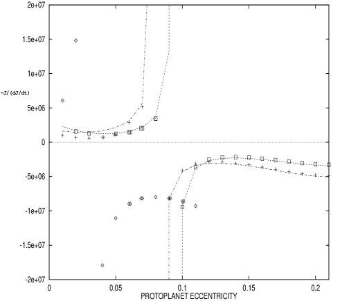
Figure 12: In this figure $t_{J}$ in yr is plotted as a function of protoplanet equilibrium eccentricity (negative values correspond to torque reversal ) for $N_{t}=1.$ The short dashed curves correspond to an assumed disc eccentricity $e=0.07$ and the short dashed long dashed curves to $e=0.05.$ The disc aspect ratio $H/r$ was taken as $0.07.$ The crosses were obtained for $e=0.05$ and $H/r=0.05,$ while the squares correspond to $e=0.07$ and $H/r=0.05.$ In the above cases disc and protoplanet orbit apsidal lines were taken to be aligned. The diamonds give $t_{J}$ for assumed antialignment and $e=H/r=0.07.$ Note the weakening of the disc interaction at the higher protoplanet eccentricities due to larger relative velocities especially in the antialigned case, to the disc.

When $e_{p}$ is significantly less than a sufficiently large disc eccentricity $e,$ the protoplanet orbital eccentricity can grow until the orbit ceases to be aligned with the disc and precesses through a full $(2\pi)$ cycle at which point it then damps. Again inward orbital migration may be reduced or reversed. Many of these features can be traced to the fact that when the equilibrium eccentricity is such that $e_{p}=e$ the situation in many ways replaces the equilibrium eccentricity solution $e_{p}=0$ in an axisymmetric disc. This we show below

Figure 13: In this figure $t_{e}$ in yr is plotted as a function of protoplanet equilibrium eccentricity (negative values correspond to circularization) for $N_{t}=1.$ The short dashed curves correspond to an assumed disc eccentricity $e=0.07$ and the short dashed long dashed curves to $e=0.05.$ The disc aspect ratio $H/r$ was taken as $0.07.$ The crosses were obtained for $e=0.05$ and $H/r=0.05,$ while the squares correspond to $e=0.07$ and $H/r=0.05.$ In the above cases disc and protoplanet orbit apsidal lines were taken to be aligned. The diamonds give $t_{e}$ for an orbit with apsidal line antialigned with that of the disc and $e=H/r=0.07.$ Note the eccentricity grows for protoplanet eccentricity less than $e$ in the aligned case while there is always decay in the antialigned case.

We use the expressions for $r,\varphi,R,$ and $\nu,$ given by equations (37), (39) in the forcing potential (38). In the case when $e=e_{p},$ and the protoplanet orbit is almost aligned with the disc with very small $|\varpi|,$ the strongest interaction occurs when $r=R,$ and $\varphi=\nu.$ This corresponds to $a=a_{p},$ and $M=\omega t+\varpi.$ Performing a first order Taylor expansion about the point of maximum interaction the forcing potential becomes

$$\Phi_{p}^{\prime}=-{Gm_{p}\over\sqrt{|(a-a_{p})^{2}+4aa_{p}\sin^{2}(M-\omega t-\varpi)+b^{2}|}}.$$ (50)

Here $|a-a_{p}|$ and $a|M-\omega t|$ are considered as small compared to $a$ and terms of order $e$ times these small quantities have been neglected. Equation (50) is to be considered in comparison to the similar expression appropriate to an axisymmetric disc

$$\Phi_{p}^{\prime}=-{Gm_{p}\over\sqrt{|(r-R)^{2}+4rR\sin^{2}(\varphi-\nu)+b^{2}|}}.$$ (51)

Given that we have already shown that $a,M$ behave just like cylindrical coordinates $(r,\varphi)$ the tidal torque calculation in an eccentric disc with $e_{p}=e$ should give the same results as an axisymmetric disc with $e_{p}=0.$ Note too that only one term should remain in the sum (42) such that $k_{1}=m,$ and $k_{2}=-m.$ Then there is zero rate of change of eccentricity. Thus the situation of aligned orbits such that $e_{p}=e$ behaves much like the case with $e_{p}=0$ in an axisymmetric disc in that it is one of steady eccentricity. The orbit then migrates at the same rate as a circular orbit in an axisymmetric disc. This is essentially what we have found on application of the torque formulae.

6.1 Numerical results

We have calculated $t_{J}/N_{t}$ and $t_{e}/N_{t}$ by summing the contributions from appropriate resonances. The normalizing factor

$$N_{t}=(r/5{\rm AU})^{-1/2}(m_{p}/(3M_{\oplus}))^{-1}(\Sigma/56)^{-1}.$$

Here the distance is measured in units of $5$ AU, the protoplanet mass in units of $3$ earth masses and the disc surface density in units of $56gmcm^{-2}.$ We have also taken the central mass to be one solar mass. The softening parameter was taken to be $b=H/\sqrt{2}.$ Our results are consistent with those of Ward(1997) in the limit where both $e$ and $e_{p}$ tend to zero. We plot $t_{J}/N_{t}$ as a function of equilibrium protoplanet orbit eccentricity $e_{p}$ for $e=0.05$ and $e=0.07,$ when disc and protoplanet apsidal lines are aligned in figure 12. Results for aspect ratios $0.05$ and $0.07$ are presented.

We plot $t_{e}$ for $N_{t}=1$ in figure 13. The trends in all cases are similar and are that for small $e_{p}$ the protoplanet eccentricity grows in the aligned case while inward migration occurs with $t_{J}\sim 2\times 10^{6}$ yr. The eccentricity growth reverses for $e_{p}\sim e$ indicating an equilibrium in accordance with the discussion above. We comment that for very small $e_{p}$ and finite $e,$ $de_{p}/dt\propto e.$ For larger $e_{p},$ $t_{J}$ and $t_{e}$ increase and $t_{J}$ eventually changes sign for $e_{p}$ exceeding $\sim 0.1.$ At these eccentricities $|t_{e}|\sim 2\times 10^{4}$ yr. We make the comment that the same dimensionless units can be used for $t_{J}$ and $t_{e}$ as for the disc models introduced in section 2 and thus the same scaling to make results applicable to different radii may be used.

In the antialigned case the disc protoplanet interaction is much weaker (see figures 12 and 13). Note too that the interaction with the disc weakens in general for larger $e_{p}$ because of the larger relative velocity of the protoplanet with respect to the disc. This results in larger values of $|t_{e}|$ and $|t_{J}|.$ Additional calculations have shown that, as expected, these values become independent of the orientation of the apsidal line when $e_{p}\gg e.$

Thus the indications are that for modest eccentricities exceeding a few $H/r$ for both disc and protoplanet the tidal interaction may differ significantly from the circular disc and small protoplanet eccentricity case. We now consider applications to the normal modes calculated in this paper.

The equilibrium protoplanet eccentricities associated with the two highest frequency modes calculated in the case of disc model A with two interior protoplanets are shown in figure 2 while those corresponding to disc model $B$ are illustrated in figure 3. These modes are associated with significant internal protoplanet eccentricities and can be thought of as giving the disc response to external forcing. Equilibrium eccentricities corresponding to the normal modes are also plotted in figures 2 and 3. These are generally larger than the disc eccentricities in the inner parts of the disc.

Equilibrium protoplanet eccentricities associated with the modes calculated in the case of disc model A with one interior protoplanet are shown in figure 8 while those corresponding to disc model $B$ are illustrated in figure 9. Equilibrium eccentricities in the case of isolated disc model $A$ are plotted in figure 10 while those corresponding to disc model $B$ are given in figure 11. In all of these cases the form of the equilibrium eccentricity curve tracks that of the corresponding normal mode according to increasing number of nodes. Thus the mode with the largest number of nodes has associated equilibrium eccentricity with the largest number of nodes.

By comparing the equilibrium eccentricities with their corresponding normal modes one sees that the modes with the smallest frequencies or pattern speeds in absolute magnitude tend to have high equilibrium eccentricities several times larger than the disc eccentricity. These correspond to the longest wavelength curves in figures 8 and 10 with corresponding modes plotted in figures 4 and 6. From our discussion above these are expected to facilitate high embedded protoplanet eccentricities. The reason the protoplanet eccentricity is significantly larger than the disc eccentricity for these modes is that, for the disc mode the effects of the nonaxisymmetric forces due to self-gravity and pressure which drive the eccentricity (see equation (18)) tend to cancel. However, the protoplanet is subject only to self-gravity with no cancelling effects from pressure forces. Therefore the equilibrium eccentricity is larger. Note that these low frequency modes are essentially disc modes and are associated with low interior protoplanet eccentricities when the latter are present. Such disc modes may also be associated with high embedded protoplanet eccentricities through secular resonances ( see section 4 above). In our models such resonances occur when the pattern speed is slightly prograde. An example is shown in figure 9. This occurs for the one protoplanet model with disc $B$ at about $20$ times the radius of the disc inner edge. Such a resonance also occurs when disc model $A$ is used but for a higher order mode at smaller radii (see figure 8).

To give numerical examples we first consider the two protoplanet model with disc $A$ as an approximation to the Upsilon Andromedae system. Taking the situation represented in figure 2 with inner boundary disc eccentricity $0.1,$ for a semi-major axis of $2.57$ AU for the outer protoplanet in the inner cavity, being $0.6$ of the inner boundary radius, $r=1.5$ corresponds to $6.4$ AU. For the mode with $\Omega_{p}=6.99\times 10^{-4}$ and disc model $A,$ $\Sigma=136gmcm^{-2}$ at $r=1.5.$ At this radius $e=0.07,$ and the equilibrium eccentricity $e_{p}=0.1.$ From figure 12 the orbital migration rate is very small and possibly outwards. We also find $|t_{e}|=10^{4}(3M_{\oplus}/m_{p})$ yr and $|(\omega_{pg}-\Omega_{p})t_{e}|\sim 30.0(M_{\oplus}/m_{p}).$ Thus in this case the eccentric disc has significant effects on the tidal torques acting on an embedded protoplanet.

The eccentricity of the outermost protoplanet orbit in the inner cavity would be $\sim 0.1.$ The currently observed value which is three or so times larger would be attained if the disc inner boundary was scaled to be at twice the outer protoplanet semi-major axis. Very similar results for the migration and circularization rates to those obtained above would still apply.

As an example to illustrate a case involving a very low frequency mode we consider the one protoplanet model with disc $A.$ The modes are plotted in figure 4 and the equilibrium eccentricities in figure 8.

For the mode with $\Omega_{p}=4.02\times 10^{-6},$ we find that at $r=10$ $e_{p}=2.5e.$ Supposing that $r=10$ corresponds to $5$ AU, $\Sigma=426gmcm^{-2}.$ From figure 12 we find that for $e=0.05,$ there is torque reversal. We also again find that $|t_{e}|\sim 3\times 10^{3}(3M_{\oplus}/m_{p})$ yr and $|(\omega_{pg}-\Omega_{p})t_{e}|\sim 30.0(M_{\oplus}/m_{p}).$

These examples indicate that protoplanets embedded in eccentric discs will be in eccentric orbits and that based on resonant torque calculations orbital migration slows down and may even reverse to become outward when the protoplanet eccentricity is sufficiently large. However, we should emphasize that these calculations are approximate and somewhat uncertain due to the cancellation of torques arising at inner and outer Lindblad resonances. To further examine the issue of protoplanet disc tidal interaction at a large eccentricity ( compared to $H/r$ and $e$) we present below a simpler calculation based on local dynamical friction which should apply in the appropriate limit and which is in essential qualitative agreement with the resonant torque calculations.

6.2 Dynamical friction calculation

We here consider the case when $e_{p}$ significantly exceeds $H/r$ but is still also significantly less than unity. This can be realized in sufficiently thin discs. In this situation the motion of the protoplanet through the disc is supersonic so we neglect pressure forces. In addition the scale of the response in both space and time becomes local ( even though the protoplanet may move globally through the disc). For example, for a length scale H, the response time scale would be $\sim H/(e_{p}r\Omega)\ll\Omega^{-1}.$

Accordingly we work in a reference frame moving instantaneously with the protoplanet in which the disc material appears to move with velocity ${\bf v}.$ Adopting local Cartesian coordinates, we suppose that the perturbing potential due to the protoplanet may be written as Fourier integral

$$\Phi_{p}^{\prime}({\bf r})=\int\Phi_{p}^{\prime}({\bf k})\exp(i{\bf k}{\bf r})d^{N}{\bf k}.$$ (52)

Here we shall consider both the two dimensional case $(N=2)$ and the three dimensional case $(N=3)$. For the two dimensional case with $\Phi_{p}^{\prime}({\bf r})=-Gm_{p}/\sqrt{r^{2}+b^{2}},$ $\Phi_{p}^{\prime}({\bf k})=-Gm_{p}\exp(-bk)/(2\pi k),$ with $k=|{\bf k}|.$ In the three dimensional case with $\Phi_{p}^{\prime}({\bf r})=-Gm_{p}/r,$ $\Phi_{p}^{\prime}({\bf k})=-Gm_{p}/(2\pi^{2}k^{2}).$

In each case, assuming a local steady state, the velocity ${\bf v}^{\prime}$ induced by the protoplanet is found from

$${\bf v}\nabla{\bf v}^{\prime}=-\nabla\Phi_{p}^{\prime}.$$ (53)

We also have

$$\nabla\cdot(D{\bf v}^{\prime})=-\nabla(\cdot D^{\prime}{\bf v}),$$ (54)

where $D$ denotes the density $(N=3)$ or the surface density $(N=2).$ In this case where only inertial terms are retained the analysis is the same as would be performed for collisionless particles ( eg Tremaine & Weinberg 1984). In this context we note that this type of calculation is also applicable to the frictional interaction with material in planetesimal form as well as with the gas disc provided the surface density and disc thickness are appropriately specified.

The rate of change of disc momentum ${\bf{\dot{P}}},$ which gives rise to a frictional force on the protoplanet acting in the direction of it’s relative velocity, may then be calculated from

$${\bf{\dot{P}}}=-\int D^{\prime}\nabla\Phi_{p}^{\prime}d^{N}{\bf r}$$ (55)

Performing an integration by parts and working in terms of the Fourier transforms of perturbations, one obtains

$${\bf{\dot{P}}}\cdot{\bf v}=-(2\pi)^{N}\int D\Phi_{p}^{\prime}({\bf k})i{\bf k}\cdot{\bf v}^{\prime}({\bf k})d^{N}{\bf k}.$$ (56)

From (53) one obtains

$${\bf v}^{\prime}({\bf k})\cdot{\bf k}={-k^{2}\Phi_{p}^{\prime}({\bf k})\over{\bf v}\cdot{\bf k}}.$$ (57)

In order to perform the integral (56) one has to apply a Landau prescription by adding an infinitessimally small negative imaginary part to the denominator ${\bf v}\cdot{\bf k}.$ One then finds

$${\bf{\dot{P}}}\cdot{\bf v}=-{\pi D(Gm_{p})^{2}\over v}{\cal Q},$$ (58)

where for $N=3,$ ${\cal Q}=4\ln(k_{max}/k_{min}),$ and for $N=2,$ ${\cal Q}=1/(2b).$ Here $(k_{max},k_{min})$ are the usual upper and lower wavenumber cut offs (eg. Tremaine & Weinberg 1984). Here reasonable values are $k_{max}=v^{2}/(Gm_{p}),$ and $k_{min}=1/H.$ The two and three dimensional cases are thus of the same form. The logarithmic factor is generally of order unity. Comparison of the two and three dimensional cases suggests that $\rho\ln(k_{max}/k_{min})=\Sigma/(8b).$ Thus the adopted softening parameter $b$ should be somewhat smaller than $H.$

Using (58) we may evaluate, remembering that ${\bf v}$ is the relative velocity between disc and protoplanet, the average rate of change of angular momentum of the protoplanet from

$$\left\langle{dJ\over dt}\right\rangle={\omega\over 2\pi}\int{\pi D(Gm_{p})^{2}({\bf r}\times{\bf v})\cdot{\hat{\bf k}}\over v^{3}}{\cal Q}dt,$$ (59)

with the integral being taken round the orbit and ${\hat{\bf k}}$ being the unit vector in the direction normal to the disc.

In the two dimensional case for $D\equiv\Sigma\propto r^{-3/2}$ one obtains for small $e_{p}$ and $e=0.$

$${1\over J}\left\langle{dJ\over dt}\right\rangle\sim{\pi m_{p}\omega\Sigma(a_{p})a_{p}^{3}\over 2be_{p}M_{*}^{2}}.$$ (60)

As this is positive it corresponds to outward migration as long as the eccentricity can be maintained. This occurs because the disc flow tends to speed up the protoplanet at apocentre where most time is spent. Numerically for $b=H/\sqrt{2}$

$${t_{J}\over N_{t}}=-2.6\times 10^{6}\left({H\over 0.07a_{p}}\right)^{2}\left({e_{p}a_{p}\over H}\right){\rm yr}.$$ (61)

While this agrees in form and is of comparable magnitude to what is obtained from resonant torque calculations (see figure 12) it is impractical to perform the latter at higher eccentricities where better agreement might be attained because of the small scale of the interaction (even at the eccentricities plotted, over $10^{6}$ resonances were included).

We may also use the above formalism to calculate the mean rate of change of orbital energy for the protoplanet to be

$$\left\langle{dE\over dt}\right\rangle=-{\omega\over 2\pi}\int{\pi D(Gm_{p})^{2}{\bf v}\cdot({\bf v}-GM_{*}r^{-1/2}{\hat{\mbox{\boldmath$\varphi$}}})\over v^{3}}{\cal Q}dt,$$ (62)

with $E=-{GM_{*}m_{p}\over 2a_{p}}$ and ${\hat{\mbox{\boldmath$\varphi$}}}$ being the unit vector in the azimuthal direction.

Performing the integration we find for small $e_{p}$ and assuming $\Sigma\propto r^{-n}$ that

$${1\over E}\left\langle{dE\over dt}\right\rangle\sim{m_{p}\omega\Sigma(a_{p})a_{p}^{3}\over 2be_{p}M_{*}^{2}}\left(4.16-7.17n\right).$$ (63)

From this we see that, for this circular disc case, the mean rate of change of orbital energy increases for $n<0.6.$ This simplified calculation indicates outward migration for density profiles that do not increase too rapidly inwards in line with the idea that the effect is caused by the interaction at apocentre.

We further comment that the more sensitive dependence on the softening parameter means that two dimensional calculations of the type carried out here, require a precise specification of this parameter that correctly represents three dimensional effects in order for them to be very accurate. Thus two dimensional torque calculations and use of torque formulae such as (43) suffer from a number of uncertainties which can be of comparable importance.

7 Discussion

In this paper we have calculated global $m=1$ modes with low pattern speed corresponding to introducing a finite disc eccentricity. An important aspect was the inclusion of self-gravity which is important for the structure of these modes as well as determining the motion of embedded protoplanets.

We considered disc models that were isolated or contained one or two protoplanets orbiting in an inner cavity. In all cases global modes were found that could be global on scales up to one hundred times the inner cavity radius. The modes could be considered as being of a type that were strongly coupled to the inner protoplanets or essentially free disc modes. In the former case the disc eccentricity could be comparable to that of the protoplanets for up to three times the outer protoplanet orbital semi-major axis with apsidal line antialigned with that of the protoplanet orbits. In the latter case the inner protoplanet orbital eccentricities were small compared to that found in the disc.

We went on to discuss the motion of a protoplanet embedded in an eccentric disc and determined, initially neglecting tidal torques, the equilibrium (non precessing) orbits which maintain apsidal alignment with the disc gas orbits. Equilibrium eccentricities were found to be comparable or possibly even exceed the disc eccentricity. In some cases secular resonance could occur producing particularly large protoplanet eccentricities.

We then formulated the calculation of the response of an eccentric disc to a protoplanet in the earth mass range in order to determine the time rate of change of the eccentricity and orbital migration rate. We found that equilibrium aligned orbits with very similar eccentricity to that of the gas disc may suffer no eccentricity change while undergoing inward migration in general. This was found from the resonant torque calculations but is also expected from direct consideration of the equations governing the tidal response. However, when the non precessing equilibrium aligned orbit has a significantly higher eccentricity than the disc, as can occur generally, but in particular for modes with very small pattern speed, orbital migration may be significantly reduced or reverse from inwards to outwards for the disc models we considered.

Attainment of high eccentricities in this way typically requires the characteristic test particle orbit precession frequency or mode pattern speed to significantly exceed the characteristic orbital circularization rate, a situation more likely for lower mass protoplanets. When tidal circularization dominates, the protoplanet equilibrium eccentricity is reduced while the apsidal line becomes significantly inclined to that of the disc. However, high protoplanet eccentricities could be excited by gravitational interactions between them (Papaloizou & Larwood 2000) and under favourable conditions this effect could act to counter tidal circularization generating significantly higher protoplanet eccentricities than that of the disc. This will be a topic for future investigation.

Although there is some uncertainty in the resonant torque calculations because of the need to sum contributions of different sign, weakening of the tidal interaction is expected on general physical grounds on account of larger protoplanet disc relative velocities at higher eccentricity. This indication of migration reversal at the higher eccentricities was found to be supported by a local dynamical friction calculation applicable in that limit. In this case the interaction near apocentre tends to speed up the protoplanet while the interaction near pericentre tends to slow it down. These effects are of opposite sign but the longer time spent near apocentre results in a net outward migration of the protoplanet for the surface density considered.

Thus the existence of global non circular motions in discs with radial excursions comparable to or exceeding the

semi-thickness may have important consequences for the migration of cores in the earth mass range. While processes of the type considered in this paper are unlikely to lead to the very high eccentricities observed for some giant planets, they may be important in controlling migration during planet formation as well as producing modest eccentricities $\sim 0.2.$

APPENDIX 1

The time averaged potential due to a perturbing inner planet

The gravitational potential per unit mass due to a planet of mass $m_{p}$ located at ${\bf r_{p}}\equiv(r_{p},\varphi_{p})$ at ${\bf r}\equiv(r,\varphi)$ is

$$\Phi=-{Gm_{p}\over\sqrt{r^{2}+r_{p}^{2}-2rr_{p}\cos(\theta)}},$$ (64)

with $\theta=\varphi-\varphi_{p}.$

In order to incorporate the effects of protoplanets orbiting interior to the disc we adopt a Jacobi coordinate system. In this system the coordinates of the innermost protoplanet are referred to the central star. The coordinates of the remainder are referred to the centre of gravity of the central mass and all interior protoplanets. The disc is referred to the centre of mass of central star and all inner protoplanets.

This has the following consequences:

For an object interior to the protoplanet with $r<r_{p},$ the acceleration of the coordinate system due to the protoplanet must be allowed for. This gives rise, correct to first order in $m_{p},$ to the indirect potential ( eg. Brouwer & Clemence 1961)

$$\Phi_{i}={Gm_{p}r\cos(\theta)\over r_{p}^{2}},$$ (65)

to be added to the potential $\Phi.$

For an object exterior to the protoplanet one must take account of the fact that the coordinate system is now based on the centre of mass of the inner protoplanets and central star. Assuming initially that $m_{p}$ is the only such protoplanet, the central potential is modified to become

$$\Phi=-{GM_{*}\over{|{\bf r}+m_{p}{\bf r_{p}}/M_{*}|}}.$$ (66)

To first order in $m_{p}$ this gives

$$\Phi=-{GM_{*}\over r}+{Gm_{p}r_{p}\cos\theta\over r^{2}}.$$ (67)

In this case too the additional potential on the right hand side of the above can be incorporated into the perturbing planet potential and viewed as giving rise to an indirect potential. Thus the form of the perturbing potential

$$\Phi=-{Gm_{p}\over\sqrt{r^{2}+r_{p}^{2}-2rr_{p}\cos(\theta)}}+{Gm_{p}rr_{p}\cos\theta\over max(r^{3},r_{p}^{3})},$$ (68)

incorporates both cases $r<r_{p}$ amd $r_{p}<r.$

In addition, although we included just one inner perturbing protoplanet, because we work to first order in their masses, the principle of linear superposition is valid such that the contributions of many such objects may be linearly superposed.

The perturbing potential due to a single protoplanet may be decomposed as a Fourier expansion in $\theta.$

Thus

$${\Phi\over Gm_{p}}=-\sum_{m=0}^{\infty}{K_{m}(r,r_{p})\over\pi(1+\delta_{m0})}\cos m\theta,$$ (69)

with

$$K_{m}(r,r_{p})=-{1\over Gm_{p}}\int^{2\pi}_{0}\Phi\cos m\theta d\theta.$$ (70)

For the problem on hand, namely the study of global $m=1$ modes of the disc planet system, we need only consider $m=0$ and $m=1.$ Then from the above

$${\pi\Phi\over Gm_{p}}=-{1\over 2}K_{0}(r,r_{p})-K_{1}(r,r_{p})\cos\theta,$$ (71)

with

$$K_{0}(r,r_{p})=\int^{2\pi}_{0}{1\over\sqrt{r^{2}+r_{p}^{2}-2rr_{p}\cos(\theta)}}d\theta$$ (72)

and

$$K_{1}(r,r_{p})=\left(\int^{2\pi}_{0}{1\over\sqrt{r^{2}+r_{p}^{2}-2rr_{p}\cos(\theta)}}\cos\theta d\theta\right.$$

$$\hskip 85.35826pt\left.-{\pi rr_{p}\over max(r^{3},r_{p}^{3})}\right).$$ (73)

Time averaged potential for a protoplanet with small eccentricity

We now suppose the protoplanet has a small eccentricity, $e_{p}$ and write for its motion $r_{p}=a_{p}(1+e_{p}\cos\omega t),\varphi_{p}=\omega t-2e_{p}\sin\omega t,$ where without loss of generality we assume the apsidal line to be along $\varphi=0$ where the displacement $\xi_{r}(r_{p})=e_{p}a_{p}$ at $t=0.$

Here the protoplanet semi-major axis is $a_{p}$ and the orbital frequency is $\omega.$

Expanding to first order in $e_{p},$ we find for the single protoplanet perturbing potential

$${\pi\Phi\over Gm_{p}}=-{1\over 2}K_{0}(r,a_{p})-{a_{p}e_{p}\over 2}{\partial K_{0}(r,a_{p})\over\partial a_{p}}\cos\omega t-$$

$$\left(K_{1}(r,a_{p})+a_{p}e_{p}{\partial K_{1}(r,a_{p})\over\partial a_{p}}\cos\omega t\right)\cos(\varphi-\omega t+2e_{p}\sin\omega t).$$

Performing the time average then gives

$${\Phi\over Gm_{p}}=-{1\over 2\pi}K_{0}(r,a_{p})-{e_{p}\over 2a_{p}\pi}{\partial(a_{p}^{2}K_{1}(r,a_{p}))\over\partial a_{p}}\cos\varphi.$$ (74)

For small $e_{p}$ we may replace $a_{p}$ by $r_{p}$ and expressing the result in terms of the radial displacement $\xi_{r}(r_{p}),$ we find

$${\Phi\over Gm_{p}}=-{1\over 2\pi}K_{0}(r,r_{p})-{\xi_{r}(r_{p})\over 2r_{p}^{2}\pi}{\partial(r_{p}^{2}K_{1}(r,r_{p}))\over\partial r_{p}}\cos\varphi.$$ (75)

From equation (75) the time averaged potential due to a protoplanet in circular orbit $(\xi_{r}(r_{p})=0)$ is

$$\Phi_{ext}=-{Gm_{p}\over 2\pi}K_{0}(r,r_{p}).$$ (76)

When $\xi_{r}(r_{p})\neq 0,$ equation (75) gives the $m=1$ component of the perturbing potential as the real part of $\Phi_{p}^{\prime}(r)\exp(i\varphi),$ with

$$\Phi_{p}^{\prime}(r)=-{Gm_{p}\xi_{r}(r_{p})\over 2\pi r_{p}^{2}}{\partial(r_{p}^{2}K_{1}(r,r_{p}))\over\partial r_{p}}.$$ (77)

APPENDIX 2

The equations of motion in two dimensional orthogonal cordinates

The basic equations of motion (1) written in vector form are

$${\partial{\bf v}\over\partial t}+{\bf v}\cdot\nabla{\bf v}=-{1\over\Sigma}\nabla\Pi-\nabla\Phi.$$ (78)

We wish to write these in component form in a general two dimensional orthogonal coordinate system $(a,\lambda)$ in the Cartesian $(x,y)$ plane as introduced in section (5). The unit vectors in these orthogonal coordinate directions are ${\bf i}_{a}=\nabla a/|\nabla a|$ and ${\bf i}_{\lambda}=\nabla\lambda/|\nabla\lambda|$ respectively. The orthogonal vertical coordinate $z$ has an additional associated orthogonal unit vector ${\bf{\hat{k}}}={\bf i}_{a}\times{\bf i}_{\lambda}.$ However, there is no dependence on $z$ and the velocity component in that direction can be taken to be zero.

Thus we may write ${\bf v}\equiv(v_{a},v_{\lambda})$ or

$${\bf v}=v_{a}{\bf i}_{a}+v_{\lambda}{\bf i}_{\lambda}.$$ (79)

To deal with equation (78), we first use the vector identity

$${\bf v}\cdot\nabla{\bf v}={1\over 2}\nabla(|{\bf v}|^{2})+{\mbox{\boldmath$\omega$}}\times{\bf v},$$ (80)

where ${\mbox{\boldmath$\omega$}}=\nabla\times{\bf v}$ is the vorticity (Arfken & Weber 2000).

Because we only wish to consider the equations in a two dimensional limit , only the $z$ component of vorticity, $\omega_{z}$ is non zero so that we may write equation (78) as

$${\partial{\bf v}\over\partial t}+\omega_{z}{\bf{\hat{k}}}\times{\bf v}+{1\over 2}\nabla(|{\bf v}|^{2})=-{1\over\Sigma}\nabla\Pi-\nabla\Phi.$$ (81)

We may now write equation (81 ) in component form using the identities (see Arfken & Weber 2000)

$$\nabla\equiv\nabla a{\partial\over\partial a}+\nabla\lambda{\partial\over\partial\lambda}$$ (82)

and

$$\omega_{z}=\left(\nabla\times{\bf v}\right)\cdot{\bf{\hat{k}}}=|\nabla\lambda||\nabla a|\left({\partial({v_{\lambda}\over|\nabla\lambda|})\over\partial a}-{\partial({v_{a}\over|\nabla a|})\over\partial\lambda}\right).$$ (83)

Doing this we obtain

$${\partial v_{a}\over\partial t}-\omega_{z}v_{\lambda}+{1\over 2}|\nabla a|{\partial(v_{a}^{2}+v_{\lambda}^{2})\over\partial a}=-{1\over\Sigma}|\nabla a|{\partial\Pi\over\partial a}-|\nabla a|{\partial\Phi\over\partial a}.$$ (84)

and

$${\partial v_{\lambda}\over\partial t}+\omega_{z}v_{a}+{1\over 2}|\nabla\lambda|{\partial(v_{a}^{2}+v_{\lambda}^{2})\over\partial\lambda}=-{1\over\Sigma}|\nabla\lambda|{\partial\Pi\over\partial\lambda}-|\nabla\lambda|{\partial\Phi\over\partial\lambda}.$$ (85)

After inserting (83) into (84) and (85) it is a simple matter to obtain equations (34) and (35) as given in section (5).