ROSAT X-ray sources in the field of the LMC

We use a sample of 50 background X-ray sources (AGN) and candidate AGN in the field of the LMC observed with more than 50 counts in archival ROSAT PSPC observations to derive the observed $\log N\ -\ \log S$ relation. We correct for the inhomogenous ROSAT PSPC exposure and the varying absorption due to the galactic and the LMC gas (for which we used an H i map derived from observations with the Parkes radio telescope). We compare the observed $\log N\ -\ \log S$ relation with a theoretical $\log N\ -\ \log S$ relation of the soft extragalactic X-ray background (SXRB) which comprises an AGN and a cluster of galaxy contribution. We find that the observed $\log N\ -\ \log S$ has a deficiency with respect to the theoretical $\log N\ -\ \log S$. There are several factors which can account for such a deficiency: (1) incompleteness of the selected AGN and cluster of galaxies sample, (2) deviation of the theoretical $\log N\ -\ \log S$ in the LMC field from the $\log N\ -\ \log S$ derived from a large sample of AGN in several fields in the sky, (3) the existence of gas additional to the H i represented in the Parkes H i map of the LMC field, restricted to the high column $\geq 10^{21}\ {\rm cm}^{-2}$ regime. We investigate the likely contribution of these effects and find that (1) a fraction (of at most $\sim$$30$%) of the AGN and clusters of galaxies in the LMC field may not have been found in our analysis and may contribute to the observed deficiency. The existence of extended regions with hot diffuse gas and source crowding makes the detection of all AGN and clusters of galaxies very difficult. (2) We cannot exclude a deviation of the $\log N\ -\ \log S$ in the field of the LMC from a mean theoretical $\log N\ -\ \log S$, especially the cluster of galaxy contribution which is of importance in the flux range we are comprising may show variations across the sky. (3) If LMC gas in addition to the H i represented in the Parkes H i map would be responsible for the deficiency and if this additional gas is restricted to the high column $\geq 10^{21}\ {\rm cm}^{-2}$ regime, and assuming that the metallicity of the ISM of the LMC is $-$0.3 dex lower than the metallicity of the galactic ISM, then a factor of $1.9\pm^{3.3}_{1.6}$ at 90% confidence of additional gas would be required which, if purely molecular, would be equal to a molecular mass fraction of $63\pm^{20}_{42}\%$. Such a value would be larger than but within the uncertainties consistent with a molecular mass fraction of $\sim$$30\%$ derived from CO observations for the high column regime of the LMC gas. From this analysis, it follows that some gas additional to the measured H i for the high column regime of the LMC gas is likely to be required to explain the observed $\log N\ -\ \log S$. But the amount of such additional gas is dependent on the completeness of our selected AGN and clusters of galaxies sample and on the assumptions made about the description of the $\log N\ -\ \log S$ of the SXRB in the field of the LMC.

1 Introduction

Recent deep X-ray studies of selected fields in the sky (with ROSAT  Chandra and XMM) have shown that the $\log N\ -\ \log S$ function of the background sources follows a canonical relation which does not differ largely across the sky. This finding is supported by the fact that at least 70–80% (and up to 90%) of the soft extragalactic X-ray background (SXRB) has been resolved into point-like X-ray sources (cf. Hasinger et al. 1998, hereafter HBG98; Hasinger et al. 2001; Giacconi et al. 2001). Most of these X-ray sources have been identified in optical follow-up programs as Active Galactic Nuclei (AGN), i.e. quasars (QSO) and Seyfert I galaxies (e.g. Schmidt et al. 1998). In addition, at higher energies (2–10 keV), a population of highly absorbed (obscured) AGN is required to explain the X-ray background (e.g. Giacconi et al. 2001 and references therein). But also clusters of galaxies, groups of galaxies and galaxies contribute to the X-ray background. They are in part contained in the sample of X-ray background sources detected in deep X-ray surveys (e.g. Rosati et al. 1995). The contribution of unobscured and obscured AGN and clusters of galaxies to the SXRB as derived from observations has been shown to be in agreement with the predictions from the standard model of the cosmic X-ray background (e.g. Gilli et al. 1999, hereafter GRS99; Gilli et al. 2001, hereafter GSH01).

Numerous ROSAT PSPC observations exist of the general field of the Large Magellanic Cloud (LMC) which allow a detailed analysis of the source statistics in the LMC region. In the present paper we will derive the observed $\log N\ -\ \log S$ of background X-ray sources in the LMC field and compare it with the $\log N\ -\ \log S$ of the SXRB. There exists an observation derived $\log N\ -\ \log S$ relation of the SXRB for the Lockman Hole field (HBG98). But we will make use of the description of the $\log N\ -\ \log S$ of GRS99 and GSH01 which comprises an AGN and a cluster component as we are investigating a large field in the sky for which the contribution of clusters of galaxies is of importance. We will make use of the description of the $\log N\ -\ \log S$ from the “fast evolution” model for the cosmic X-ray background (see Sec. 2 for a presentation of the description of the $\log N\ -\ \log S$ discussed and used in this paper). One of our goals is to derive constraints for the gas between us and the X-ray sources, in particular for the gas of the LMC. Clearly the statistics of the sources detected is influenced by the absorption by intervening gas but it is also influenced by the detection capabilities related with the nature of the ROSAT PSPC.

The sample of AGN and candidate AGN has been set up in Kahabka (2001, hereafter Paper II) and is based on the ROSAT PSPC catalog of Haberl & Pietsch (1999, hereafter HP99). For this AGN sample we will construct in Sect. 3 and 4 the $\log N\ -\ \log S$ which we will correct for the variable exposure, the absorption due to the variable LMC $N_{\rm H}$ and also for the incompleteness of AGN observed in the sample with a certain number of counts in the source circle. The latter incompleteness is due to spatial background variations across the merged observations and the requirement for the detection of an AGN of an at least $4\sigma$ excess of the source counts above the background in the source circle.

We will derive constraints on the LMC gas additional to the H i which apparently are required to get agreement between the $\log N\ -\ \log S$ derived in this work and the $\log N\ -\ \log S$ of the SXRB inferred in fields with very low absorbing columns. We also will allow the cluster contribution in the theoretical $\log N\ -\ \log S$ to vary and investigate the effect on the constraints for the LMC gas additional to the H i. In Sect. 5 we will derive constraints on the amount of molecular gas under the assumption that the gas additional to the H i is molecular. In addition we will estimate the effect of obscuration of the sky in the LMC field by dark clouds.

2 The theoretical log N – log S

From deep X-ray observations in fields at a high galactic latitude it has been found that the $\log N\ -\ \log S$ can be well described by a powerlaw with different slopes above and below a flux $S_{\rm b}$ (cf. Hasinger et al. 1993; HBG98). For fluxes (0.5 – 2.0 keV) above $S_{\rm b}=2.66\ 10^{-14}\ {\rm erg}\ {\rm cm^{-2}}\ {\rm s^{-1}}$ the differential number of sources per flux interval $dN/dS=n(S)$ has been determined by HBG98 as

$$n(S)=n_{1}\ S_{\small 14}^{-b_{1}}$$ (1)

with $n_{1}=238.1$ and $b_{1}=2.72$. Similar values for $n_{1}$ and $b_{1}$ are given in Hasinger et al. (1993). The flux $S_{14}$ is given in units of $10^{-14}\ {\rm erg}\ {\rm cm^{-2}}\ {\rm s^{-1}}$. From this relationship the number $N(>S)$ of sources per square degree and with fluxes in excess of a given flux $S$ can be determined from

$$N(>S)=138.4\ S_{\small 14}^{-1.72}$$ (2)

For fluxes (0.5 – 2.0 keV) below $S_{\rm b}$ $N(>S)$ is given by

$$N(>S)=118.1\ S_{\small 14}^{-0.94}\ -21.36$$ (3)

This description of the $\log N\ -\ \log S$ has been derived from deep observations of a small field of 1.4 square degrees in the sky with low galactic absorbing columns (the Lockman Hole).

Optical identifications of this sample by Schmidt et al. (1998) have shown that a large fraction of the X-ray sources is AGN. Other objects in this sample are clusters of galaxies and a few foreground stars. The contribution of AGN, clusters of galaxies and groups of galaxies to the $\log N\ -\ \log S$ requires a more detailed modeling of the $\log N\ -\ \log S$. In addition it has to be taken into account that clusters of galaxies and galaxy groups may show variations across the sky (cf. Giuricin et al. 2000). For fluxes above $10^{-14}\ {\rm erg}\ {\rm cm^{-2}}\ {\rm s^{-1}}$ the contribution of galaxy clusters becomes important (cf. GRS99).

Even for fluxes above $\sim$$10^{-13}\ {\rm erg}\ {\rm cm^{-2}}\ {\rm sec^{-1}}$ besides AGN clusters of galaxies are already an important contribution to the $\log N\ -\ \log S$. As the $\log N\ -\ \log S$ derived for the Lockman Hole field does not extend to fluxes in excess of $\sim$$10^{-13}\ {\rm erg}\ {\rm sec^{-1}}$ (cf. HBG98) the fraction of clusters contained in this field is small ($\sim$$11\%$, cf. Lehmann et al. 2001).

A more sophisticated model for the description of the SXRB is required for samples derived from larger fields which extend over at least a few square degrees as the cluster contribution to the $\log N\ -\ \log S$ is of importance.

Following the description of GRS99 we used in addition to the $\log N\ -\ \log S$ the “flattened” $\log N\ -\ \log S$ which is the $\log N\ -\ \log S$ modified by a scaling factor $S_{14}^{1.5}$ ($S_{14}$ is the flux in units of $10^{-14}\ {\rm erg}\ {\rm cm^{-2}}\ {\rm s^{-1}}$). The Euclidean slope for such a $\log N\ -\ \log S$ would become horizontal.

From Fig. 3 of GRS99 we derived an analytical presentation of the cluster component:

$$N(>S)_{\rm Cluster}=1.7\times\frac{(2+\log(S_{\small 14}))^{2.4}}{{S_{\small 14}}^{1.5}}$$ (4)

This presentation of the cluster $\log N\ -\ \log S$ is in the flux range $10^{-14}\ {\rm erg}\ {\rm cm}^{-2}{\rm sec}^{-1}$ to $10^{-11}\ {\rm erg}\ {\rm cm}^{-2}{\rm sec}^{-1}$ in good agreement with the cluster $\log N\ -\ \log S$ derived by Rosati et al. (1995) and De Grandi et al. (1999).

In order to be consistent with the $\log N\ -\ \log S$ of GRS99 we also reproduced the AGN $\log N\ -\ \log S$ from the same Figure (but we will derive another description for the AGN component to which we will refer later on). We derive the following analytical presentation (which is a reasonable approximation in the flux range $10^{-15}$ to $10^{-11}\ {\rm erg}\ {\rm cm}^{-2}\ {\rm sec}^{-1}$).

$$N(>S)_{\rm AGN}=32\times(\log(120\times S_{\small 14}))^{1.1}\times(S_{\small 14})^{-1.7}$$ (5)

Recently the “flattened” $\log N\ -\ \log S$ extending over the flux range $10^{-10}$ to $10^{-15}$ ${\rm erg}\ {\rm cm}^{-2}\ {\rm s}^{-1}$ (and below) has been derived from a sample of $\sim$$700$ AGN by Miyaji et al. (2000). From such a large AGN sample extending over such a large flux range constraints have been derived for the cosmological evolution of the soft X-ray selected AGN as a function of the redshift. There are two main models, pure luminosity evolution (PLE) with redshift and a luminosity dependent density evolution (LDDE) with redshift. The latter model has been found to be consistent with recent observational data and is referred to as the “standard model” (e.g. GRS99). It is “model A” of GSH01. This model has been further refined by GSH01 by allowing type 2 AGN to evolve faster than type 1 AGN (“fast evolution” and “model B” of GSH01). Type 1 and type 2 AGN are in the unification scheme of AGN related due to the orientation (with respect to the observer) of a molecular torus surrounding the nucleus of the AGN: Type 1 is not obscured while type 2 is obscured.

We derived rough analytical representations of the “flattened” $\log N\ -\ \log S$ for the standard model (A) and the model with fast evolution (B) by making a fit to the $\log N\ -\ \log S$ in the flux range $10^{-15}$ to $10^{-10}\ {\rm erg}\ {\rm cm}^{-2}\ {\rm s}^{-1}$. But the fit is less accurate for the extreme flux ranges around $10^{-10}$ and $10^{-15}\ {\rm erg}\ {\rm cm}^{-2}\ {\rm s}^{-1}$ respectively. For model (A,B) we used the following analytical representation

$$S_{14}^{1.5}\ N(>S)_{\rm AGN}=F(S)^{A,B}\times G(S)^{A,B}$$ (6)

with

$$F(S)^{A,B}=a_{1}\times(S_{\small 14})^{a_{2}}$$ (7)

and

$$G(S)^{A,B}=C^{A,B}\left\{\begin{array}[]{r@{\quad:\quad}l}e^{-\frac{(\log(S_{\small 14})-a_{5})^{2}}{2(a_{3})^{2}}}&\log(S_{\small 14})<a_{5}\\ e^{-\frac{(\log(S_{\small 14})-a_{5})^{2}}{2(a_{4})^{2}}}&\log(S_{\small 14})\geq a_{5}\\ \end{array}\right.$$ (8)

with

$$C^{A,B}=\frac{10}{\sqrt{2\pi}}\left\{\begin{array}[]{r@{\quad:\quad}l}a_{3}/a_{4}&\log(S_{\small 14})<a_{5}\\ 1/a_{4}&\log(S_{\small 14})\geq a_{5}\\ \end{array}\right.$$ (9)

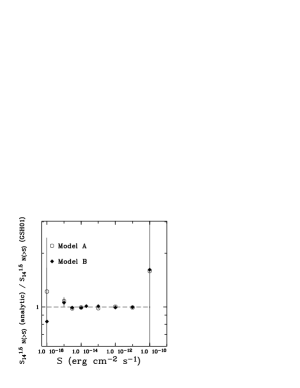
Figure 1: Ratio between the analytical presentation and the theoretical model for the “flattened” $\log N\ -\ \log S$. The theoretical model (A and B) is taken from Fig. 3 of GSH01. The analytical presentation is given in Eq. 6 to 9. The errors given for the points of the model function are the errors used for the least-square fit and are arbitrary. For typical errors of observational data points see Fig. 3 of GSH01.

The parameters $\rm a_{1}$, $\rm a_{2}$, $\rm a_{3}$, $\rm a_{4}$ and $\rm a_{5}$ have been determined from a least-square fit to the curves given in Fig 3 of GSH01 for model A and model B and are given in Table 1.

Table 1: Parameters $a_{1}$, $a_{2}$, $a_{3}$, $a_{4}$ and $a_{5}$ for model A and model B of the function $S_{\small 14}^{1.5}\ N(>S)$.

Model	$a_{1}$	$a_{2}$	$a_{3}$	$a_{4}$	$a_{5}$
A	109.42	$-$1.581	2.24	12.19	0.312
B	100.2	$-$1.565	2.2	12.44	0.45

From Eq. 4 and Eq. 6 to 9 we can derive the fractional contribution of cluster of galaxies to the accumulative number of sources. The fraction of clusters of galaxies to the total accumulative source number extends from $\sim$47% to 12% for the flux range of $10^{-12}$ to $10^{-14}\ {\rm erg}\ {\rm cm}^{-2}{\rm s}^{-1}$ respectively (cf. Tab. 2).

Table 2: Cluster to total and cluster to AGN ratio for a given limiting flux using Eq. 4 and Eq. 6–9, model B.

$\log$ flux	$\frac{\rm Cluster}{\rm Cluster+AGN}$	$\frac{\rm Cluster}{\rm AGN}$
(${\rm erg}\ {\rm cm}^{-2}\ {\rm s}^{-1}$)
$-12$	0.469	0.883
$-13$	0.269	0.367
$-14$	0.118	0.133
$-15$	0.060	0.064

In Sect. 4 we will apply this analytical description of the “flattened” $\log N\ -\ \log S$ for the model with fast evolution (B) to the observed $\log N\ -\ \log S$ relation. We note that with the quality of our data we cannot decide between model A and B. In Fig. 1 we give the ratio of the analytical presentation of the $\log N\ -\ \log S$ making use of Eq. 6 to 9 and of the data points taken from GSH01.

3 The completeness correction

We will discuss effects which determine the incompleteness of the $\log N\ -\ \log S$ distribution of the AGN sample, the inhomogenous PSPC exposure across the observed LMC field, the variable absorption due to galactic and LMC gas, and the confusion of counts in the source circle due to the observation intrinsic background. In Sec. 4 we will correct the observed $\log N\ -\ \log S$ for these incompleteness effects and compare it with a theoretical $\log N\ -\ \log S$ of the soft extragalactic X-ray background.

3.1 PSPC exposure depth

The merged exposure varies for the LMC field in the range $\sim$(0.6-168) ksec. For the AGN given in Paper II it follows that an unabsorbed flux of $10^{-12}\ {\rm erg}\ {\rm cm^{-2}}\ {\rm s^{-1}}$ in the (0.5 – 2.0) keV band equals a count rate of $\sim$$0.1\ {\rm s}^{-1}$ in the same energy band. Such a value is similar to the count rate of $0.074\ {\rm s}^{-1}$ derived from a simulation of an unabsorbed AGN type spectrum.

We have considered for the $\log N\ -\ \log S$ analysis only AGN, for which at least 50 counts have been collected in the source circle making use of the merged observations. We assume that such an AGN sample is complete. The correctness of this assumption can be confirmed from inspection of the counts histogram derived from the observed AGN sample and independently derived from a simulated AGN sample (cf. Fig. 2).

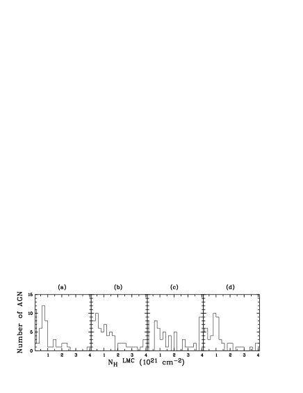
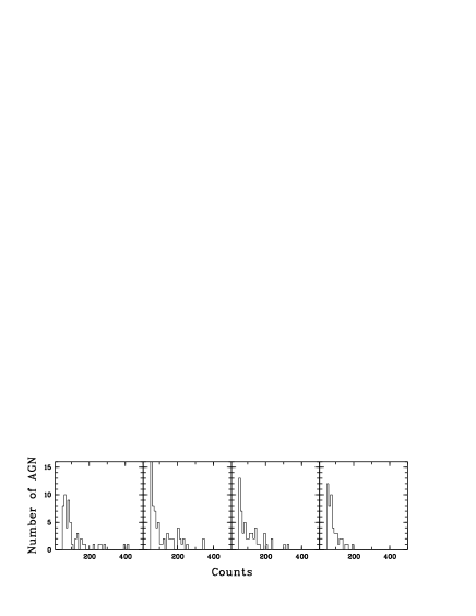
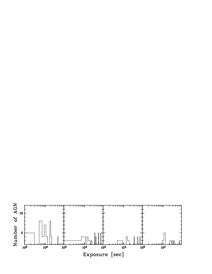
Figure 2: Distribution of LMC hydrogen absorbing column density (upper panel), the counts (middle panel) and the exposure (lower panel) of the observed (panel (a)) and simulated (panel (b) to (d)) AGN sample in the investigated LMC field. The samples have been selected for $>$50 source counts and have sizes of 50, 71, 57, and 52 sources respectively. The simulated samples are drawn from a sample using an H i map which has $N_{\rm H}=\hbox{H\,{\sc i}}\$ (b) and which is scaled in the high column $N_{\rm H}>10^{21}\ {\rm cm}^{-2}$ regime by a factor of two (c) respectively. For the simulated sample (d) the cluster scaling factor has been set to 0.2 and an H i map has been used with $N_{\rm H}=\hbox{H\,{\sc i}}\$.

For a given flux an AGN needs a minimum exposure $E_{min}$ to give the required 50 counts. This minimum exposure would be

$$E_{min}=\frac{675\leavevmode\nobreak\ s}{S_{12}}$$ (10)

with $S_{12}$ the flux in units of $10^{-12}$ ${\rm erg}\ {\rm cm}^{-2}\ {\rm s}^{-1}$. From this equation, it follows that all AGN with fluxes above $10^{-12}\ {\rm erg}\ {\rm cm^{-2}}\ {\rm s^{-1}}$ should be contained in our $\log N\ -\ \log S$ distribution as they require only a 675 sec exposure to be detected. It also follows that faint AGN with a flux of $10^{-14}\ {\rm erg}\ {\rm cm^{-2}}\ {\rm s^{-1}}$ would need an exposure of at least 67 ksec.

3.2 Varying H i absorption

A second effect which contributes to the incompleteness of the observed AGN sample is the variable absorption due to the galactic and LMC gas. Such an absorption further reduces the counts observed from the AGN and the fraction of detected AGN for a given flux. In the region of the LMC both the galactic and the LMC absorbing H i columns show a large variation (cf. Brüns et al. 2001). The largest hydrogen absorbing columns due to LMC gas ($>10^{21}\ {\rm cm}^{-2}$) are observed in the eastern cloud complex of the LMC. In these regions ROSAT PSPC observations with a deep exposure exist.

We proceeded in the same way as we did when we calculated the incompleteness due to the variable exposure across the LMC field. We determined for each pixel of the merged exposure map the local $N_{\rm H}$ due to the LMC gas and we added a constant value for the absorption due to the galactic foreground gas of $N_{\rm H}=5\times 10^{20}\ {\rm cm}^{-2}$. We determined a reduced effective exposure by correcting for the absorption due to LMC gas ($N_{\rm H}$ in units of $10^{21}\ {\rm cm}^{-2}$) and due to galactic gas (with a column of $5.\ 10^{20}\ {\rm cm}^{-2}$). From simulations we determined the conversion factor $f_{\rm c(band)}=\frac{flux({\rm erg}\ {\rm cm}^{-2}\ {\rm s}^{-1})}{countrate}$. The count rate to flux conversion factor is used to convert the source count rate to the intrinsic unabsorbed source flux. This flux is used to construct the $\log N\ -\ \log S$. For a photon spectrum with a powerlaw index $-\Gamma=2.0$ and a LMC metallicity ($-$0.3 dex) we found for the (0.1 – 2.4 keV) band

$$f_{\rm c(0.1-2.4)}=1.0\times 10^{-11}+1.64\times 10^{-10}\big{(}(N_{\rm H}+3.9)/20\big{)}^{1.4}$$ (11)

and for the spectrally hard (0.5 – 2.0 keV) energy band

$$f_{\rm c(0.5-2.0)}=5.7\times 10^{-12}+7.7\times 10^{-11}\big{(}(N_{\rm H}+3.9)/20\big{)}^{1.4}$$ (12)

Independently we found from simulated unabsorbed ROSAT PSPC spectra with a powerlaw photon index $-\Gamma=2.0$, that the intrinsic flux in the spectrally hard band $f_{c(0.5-2.0)}(N_{\rm H}=0)$ can be determined from the intrinsic flux in the spectrally broad band $f_{c(0.1-2.4)}(N_{\rm H}=0)$ as

$$\frac{f_{c(0.5-2.0)}(N_{\rm H}=0)}{f_{c(0.1-2.4)}(N_{\rm H}=0)}=0.437$$ (13)

(a ratio changing to 0.374, 0.311 and 0.157 for powerlaw slopes $\Gamma$ of –2.2, –2.4 and –3.0 respectively). We determined the effective reduced exposure $E_{\rm r}$ from the uncorrected exposure $E$ from the equation

$$E_{\rm r}={\frac{f_{c}(N_{\rm H}=0)}{f_{c}(N_{\rm H})}}\times E$$ (14)

Due to absorption by gas in the line of sight to an AGN less counts are observed compared to an AGN which is not absorbed. This is equivalent to a reduced exposure. We determined the LMC $N_{\rm H}$ from an H i map measured with the Parkes telescope. This map has been aligned using reference points. Furthermore we took the variable galactic $N_{\rm H}$ into account. We determined the galactic $N_{\rm H}$ from the map of Dickey & Lockman (1991). We determined the flux conversion factor for individual AGN by evaluating the Parkes 21-cm map for the galactic foreground gas. As the count rate to flux conversion factors (cf. Eq. 11 and 12) have been derived for a galactic column of $5\times 10^{20}\ {\rm cm^{-2}}$ we only considered the net extra galactic $N_{\rm H}^{\rm gal\ net}\ =N_{\rm H}^{\rm gal}-5\ 10^{20}\ {\rm cm^{-2}}$.

We did not correct the H i values for the LMC gas for self-absorption. But the correction factors for self-absorption of the SMC H i have been given by Stanimirovic et al. (1999) and from a preliminary analysis of the $\log N\ -\ \log S$ of background X-ray sources in the field of the SMC we found that consideration of self-absorption has only a small effect on the corrected $\log N\ -\ \log S$.

We also derived from simulations analytical expressions to correct the observed PSPC count rates into fluxes by taking the absorption due to galactic and LMC gas into account. In the upper panel of Fig. 3 we give the incompleteness (due to the exposure and the absorption by the H i gas) of the sample of AGN in the field of the LMC which have been observed with more than 50 counts. We give the fraction of observed AGN as a function of the flux (0.5 – 2.0 keV) corrected for the absorption due to the intervening galactic and LMC gas.

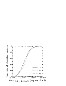
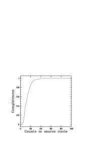
Figure 3: Upper panel: The completeness of the AGN sample as a function of the flux and due to the variable merged exposure and the variable absorption due to the LMC gas in the observed LMC field. The fraction of AGN at a given flux and observed with at least 50 counts is given for LMC absorbing columns which are scaled by a factor of 1.0, 2.0, and 3.0 respectively. Lower panel: The completeness of the AGN sample in the LMC field as a function of the counts in the source circle. The completeness has been determined from the 4$\sigma$ excess in counts in the source circle measured from the merged smoothed background image of the observations.

3.3 Background confusion

A third effect which contributes to the incompleteness of the selected AGN sample is the confusion of counts in the source circle by counts due to the background. We created a merged background image with a binsize of 1.′25 from all background images constructed in the spectrally hard band and retrieved from the public ROSAT archive. Only observations made in the field of the area of the LMC for which the $\log N\ -\ \log S$ has been derived have been used. We restricted the analysis to the inner 20′ of the field of view. We constructed the histogram in the 4$\sigma$ excess counts from all observations and we determined from this histogram the probability that a source with a given number of counts will be detectable in one of the considered observations. The completeness of the selected AGN sample as a function of the measured counts is given in the lower panel of Fig. 3. It follows that for 50 counts the completeness of the AGN sample is 100% and for 20 counts $\sim$85%.

Part of the observed background is due to extended hot diffuse gas in the LMC. In these regions it is difficult to detect background AGN due to confusion with emission from hot extended gas. Such regions have to be excluded from the analysis. There is a way to take this effect into account. By counting the number of counts from diffuse emission $NCD$ in a cell of the size of the source radius one can decide whether a source with $NCS$ counts is detectable with more than $\Sigma$ sigma. Using Poissonian statistics one finds such a source is detectable only in regions where the number of diffuse counts follows the relation

$$NCD<(\frac{NCS}{\Sigma})^{2}$$ (15)

If we set a significance threshold of $4\sigma$ and a size of the source cell of $100\arcsec\times 100\arcsec$ then an AGN with 50 counts can only be detected in regions with less than 156 diffuse counts in the source radius. We thus excluded from the $\log N\ -\ \log S$ analysis regions of the LMC where more than 156 diffuse counts are detected in the spectrally hard (0.5 – 2.0 keV) band and considered the merged exposure of the inner 20′ of the detector. This region is located around the 30 Dor complex (cf. Fig. 4).

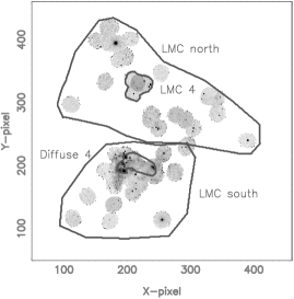
Figure 4: The regions LMC north, LMC south, and LMC 4, which have been used for the $\log N\ -\ \log S$ analysis are marked with dark lines. Also given is the region of extended diffuse emission Diffuse 4 in the 30 Dor complex which has been excluded from the analysis.

4 The fit of the observed log N – log S

For a threshold of 50 counts for the AGN sample given in Paper II, 53 AGN are found in the field of the LMC. If we exclude the region of extended diffuse emission Diffuse 4 then we find 50 AGN in the same field. We will apply the $\log N\ -\ \log S$ analysis in the LMC field to this sample of 50 AGN. But we will choose a lower threshold of 30 counts for the $\log N\ -\ \log S$ analysis applied to the AGN sample derived for the field of the Supergiant Shell LMC 4. We constructed, for the sample of 50 AGN, the observed $\log N\ -\ \log S$ which we corrected for the incompleteness due to the varying exposure depth, the varying absorption due to the galactic and LMC H i gas, and for background confusion. We excluded the extended region of hot diffuse gas in the 30 Dor complex. We derived the $\log N\ -\ \log S$ function from the count rates measured in the spectrally hard and broad band. But in the $\log N\ -\ \log S$ function the flux has always been corrected to that of the spectrally hard band in order to allow a direct comparison.

In Fig. 5a we show for the AGN sample the uncorrected $\log N\ -\ \log S$ relation in the spectrally hard band. In the further investigation we always will show the $\log N\ -\ \log S$ in the spectrally hard band. We now can assume that the discrepancy between the observed $\log N\ -\ \log S$ and the standard $\log N\ -\ \log S$ shows us the incompleteness due to exposure depth and H i absorption variations.

Figure 5: $\log N\ -\ \log S$ of the classified AGN sample in the LMC field derived from the observed count rates in the spectrally hard (0.5 – 2.0 keV) band for off-axis angles $<$19.′5. The chosen sample of AGN is complete for $\geq 50$ counts. (a) The $\log N\ -\ \log S$ has not been corrected for incompleteness. (b) The $\log N\ -\ \log S$ has been corrected for incompleteness due to the exposure and the absorbing galactic and LMC gas assuming $N_{\rm H}=N_{\rm HI}$. (c) The $\log N\ -\ \log S$ corrected for incompleteness due to the variable exposure across the LMC field and corrected for the incompleteness due to absorption by galactic and LMC gas (the H i) across the field but with the LMC $N_{\rm H}$ scaled by a factor 3.2. The thin solid histogram gives the theoretical $\log N\ -\ \log S$ (model B of GSH01) and the arrow marks the lower flux threshold used in the least-square fit.

We assume that we have considered all AGN at a given flux which have been detected with at least 50 counts. From inspection of Fig. 3 it follows that the completeness of our AGN sample is expected to be better than 90% for fluxes above $10^{-12}\ {\rm erg}\ {\rm cm}^{-2}\ {\rm sec}^{-1}$. For fluxes of $10^{-12}$ to $10^{-13}\ {\rm erg}\ {\rm cm}^{-2}\ {\rm sec}^{-1}$ the incompleteness should be not larger than a factor of three while at the low flux end of $10^{-14}\ {\rm erg}\ {\rm cm}^{-2}\ {\rm sec}^{-1}$ the observed AGN sample is complete to less than 10%.

The $\log N\ -\ \log S$ corrected for the variable exposure and the H i absorption is given in Fig. 5b. Surprisingly it is found that this $\log N\ -\ \log S$ corrected for the variable exposure in the LMC field and the variable intervening galactic and LMC gas is below the $\log N\ -\ \log S$ of the SXRB (e.g. using the description from model B of GSH01). There could be several reasons for this discrepancy.

a) There is the possibility of the existence of gas additional to the (galactic and LMC) H i derived from a Parkes 21-cm survey of the field of the LMC. Such additional gas which is not reproduced in the H i data may be in the form of atomic or molecular gas. In Sect. 5.2 of Kahabka et al. (2001, hereafter Paper I) we have investigated likely systematic effects to derive H i columns with the Parkes beam compared with a much narrower beam (the ATCA beam). We investigated the gas of the Small Magellanic Cloud (SMC) and we found that for H i columns below $\sim$$3.5\ 10^{21}\ {\rm cm^{-2}}$ the H i columns may be systematically underestimated by $\sim$$(5-15)\%$. The additional gas aspect will be explored in Sect. 4.1.

b) There is also the possibility that the $\log N\ -\ \log S$ in the field of the LMC deviates from the $\log N\ -\ \log S$ of the SXRB. The $\log N\ -\ \log S$ is in our description from Sect. 2 composed of two components, an AGN and a cluster component. We here assume that the description of the AGN component is according to model B of GSH01. The cluster component of the $\log N\ -\ \log S$ which we derive from GRS99 will in Sect. 4.2 be allowed to vary. We introduce a scaling factor for the cluster component and we explore the constraints on the LMC gas and the $\log N\ -\ \log S$.

4.1 Constraining intervening LMC gas columns

Assuming there exists additional gas in the line of sight towards the AGN which is not contained in the used H i column density map and which has not been accounted for in constructing the $\log N\ -\ \log S$, we can rescale the H i value in the direction towards the AGN, thus constrain such additional gas from a least-square fit (of the observed $\log N\ -\ \log S$ compared to a theoretical $\log N\ -\ \log S$). We simplified the numerical effort as we applied it only to H i columns in excess of $10^{21}\ {\rm cm}^{-2}$. We also used a threshold of 50 source counts.

Other systematic effects which we will take into account in this section are due to differences in the abundance models and in the AGN spectral models. There exist different abundance models for the interstellar medium (ISM). Also the details of the metal abundance in LMC gas are not accurately known. The average metallicity of LMC gas is, however, known to be approximately $-0.3$ dex below the galactic metallicity (de Boer 1991; Russell & Dopita 1992). To calculate the absorption of X-rays the total metal content is needed, irrespective of the split between gas-phase and dust-depleted metals. Originally, models were based on the metallicity scale of Morrison & McCammon (1983, MM). Recently Wilms, Allen & McCray (2000, WAM) have updated the photoabsorption cross sections in the X-ray regime. In addition they have presented a set of abundances for the ISM taking the gas and the dust phase into account. We will make use of the abundance models of MM and WAM and we will assume for the LMC gas a mean metallicity of $-$0.3 dex.

Table 3: Count rate to flux conversion factors for models with different sets of abundances. We give for each model the abundances $A_{\rm Z}$ for element $Z$ in the nomenclature $12+\log A_{\rm Z}$. We give the count rate to flux conversion factors $f_{\rm c}$ for the spectrally hard and the spectrally broad ROSAT PSPC band. The conversion factor $f_{\rm c}$ is determined by the equation $f_{\rm c}=10^{-11}\times(f_{1}+f_{2}\times(N_{\rm H}+3.9)/20)^{1.4})$. The coefficients $f_{1}$ and $f_{2}$ are given for each model and each spectral band.

	$-\Gamma$	$A_{\rm Z}$	$f_{1}$	$f_{2}$
Model			broad (0.1 – 2.4 keV)
Ba	2.0	MM	1.00	16.4
Bb	2.0	WAM	1.45	12.8
Bc	2.2	MM	1.00	20.5
Bd	2.2	WAM	1.50	16.2
Be	2.4	MM	1.00	26.0
Bf	2.4	WAM	1.70	20.5
Model			hard (0.5 – 2.0 keV)
Ha	2.0	MM	0.57	7.7
Hb	2.0	WAM	0.77	6.0
Hc	2.2	MM	0.52	8.2
Hd	2.2	WAM	0.70	6.5
He	2.4	MM	0.46	8.7
Hf	2.4	WAM	0.70	6.8

In the notation for the model, (B) and (H) refer to the broad and hard spectral band respectively, (a,c,e) and (b,d,f) for the abundance model of MM and WAM respectively (with MM, Morrison & McCammon, 1983, and $-$0.3 dex for LMC abundances (C=8.35, N=7.39, O=8.57, Ne=7.84, Na=6.02, Mg=7.30, Al=6.19, Si=7.27, S=6.98); WAM, Wilms, Allen, & McCray, 2000, and $-$0.3 dex for LMC abundances (C=8.08, N=7.58, O=8.39, Ne=7.64, Na=5.86, Mg=7.10, Al=6.03, Si=6.97, S=6.79). In addition a,c,e (and b,d,f) refer to $-\Gamma$ values of $2.0,2.2$, and $2.4$ respectively.

The count rate to flux conversion factor $f_{\rm c}$ derived from simulations in Sec 3.2 depends on the chosen set of abundances. We here derived $f_{\rm c}$ for the set of abundances of Morrison & McCammon (1983) and WAM, cf. Tab. 3.

The flux distribution of AGN can, in most cases, be described by a powerlaw model in the energy range of the ROSAT PSPC. The photon powerlaw index $\Gamma$ covers values which lie in a narrow range (cf. Paper I). The mean value of $-\Gamma$ is $\sim$2.2 with a 1$\sigma$ deviation of $\sim$0.2. In several investigations it has been found that AGN type spectra cover a narrow range in $\Gamma$ with the “extreme” range of $-\Gamma$ values extending from $2.0$ to $3.0$ respectively (cf. Brinkmann et al. 2000, and discussion in Paper I). The count rate to flux conversion factor $f_{\rm c}$ has in addition been derived for spectral models with powerlaw indices in the range $-\Gamma=(2.0-3.0)$, cf. Tab. 3.

We restricted the further $\log N\ -\ \log S$ analysis to the abundance models and the models for the AGN spectral flux distribution given in Tab. 3. In addition, the flux conversion factors have been calculated for two different spectral bands, the hard (0.5 – 2.0 keV) and the broad (0.1 – 2.4 keV) band. We applied a least-square fit to the observed $\log N\ -\ \log S$ which has been corrected for incompleteness and assuming different sets of conversion factors.

The gas fractions additional to the H i constrained from a least-square fit to the $\log N\ -\ \log S$ of background X-ray sources in different areas of the LMC field are given in Table 4. In Column (1) of the table the field designation is given, in Column (2) the area of the field, in Column (3) the spectral model used, in Column (4) the counts threshold, in Column (5) the used flux range, in Column (6) and (7) the number of AGN considered (in the whole and high column regime of the LMC gas), in Column (8) the gas fraction additional to the H i derived from the least-square fit, and in Column (9) the reduced chi-squared of the fit. The result for additional gas averaged over the different models and derived for the spectrally hard band is in the range $N_{\rm H}^{\rm LMC}=1.9\pm^{3.3}_{1.6}\ \hbox{H\,{\sc i}}$. The amount of gas in excess of the observed H i derived for the spectrally broad band is $N_{\rm H}^{\rm LMC}=1.5\pm^{3.7}_{1.1}\ \hbox{H\,{\sc i}}$.The adjusted $\log N\ -\ \log S$ derived from the classified AGN sample making use of the spectrally hard flux is given in the lower panel of Fig. 5. We obtained a generally good match with the standard $\log N\ -\ \log S$ relation.

Table 4: Fraction $n$ of gas additional to the H i in the high column ($>10^{21}\ {\rm cm^{-2}}$) regime derived from a $\log N\ -\ \log S$ analysis for different fields in the LMC (90% confidence). The designation for the field (cf. Table 3), the area of the field, the spectral model (cf. Table 3), the counts threshold, the flux range, the number of AGN used in the $\log N\ -\ \log S$ analysis, and the reduced $\chi^{2}$ and the degrees of freedom (DOF) are given.

Field	Area	Model	Counts	Flux	Number		gas	$\chi^{2}_{\rm red}$/DOF
			threshold	range	AGN		fraction
	($\Box$∘)			(log (${\rm erg}\ {\rm cm^{-2}}\ {\rm s}^{-1}$))	(a)	(b)	n
LMC field	15.2	Ha	50	(-13.8,-11.0)	50	16	1.8$\pm^{3.4}_{1.6}$	0.42/20
LMC field	15.2	Hb	50	(-13.8,-11.0)	50	16	2.4$\pm^{3.0}_{1.8}$	0.44/20
LMC field	15.2	Hc	50	(-13.8,-11.0)	50	16	1.6$\pm^{3.4}_{1.4}$	0.42/20
LMC field	15.2	Hd	50	(-13.8,-11.0)	50	16	2.2$\pm^{3.2}_{1.8}$	0.37/20
LMC field	15.2	He	50	(-13.8,-11.0)	50	16	1.4$\pm^{3.2}_{1.4}$	0.47/20
LMC field	15.2	Hf	50	(-13.8,-11.0)	50	16	2.0$\pm^{3.4}_{1.6}$	0.44/20
LMC field	15.2	Ba	50	(-13.8,-11.0)	50	16	1.4$\pm^{3.8}_{1.0}$	0.50/21
LMC field	15.2	Bb	50	(-13.8,-11.0)	50	16	1.8$\pm^{3.6}_{1.2}$	0.55/21
LMC field	15.2	Bc	50	(-13.8,-11.0)	50	16	1.2$\pm^{3.8}_{1.0}$	0.45/21
LMC field	15.2	Bd	50	(-13.8,-11.0)	50	16	1.8$\pm^{3.6}_{1.2}$	0.61/21
LMC field	15.2	Be	50	(-13.8,-11.0)	50	16	1.4$\pm^{3.6}_{1.2}$	0.50/20
LMC field	15.2	Bf	50	(-13.8,-11.0)	50	16	1.6$\pm^{3.8}_{1.0}$	0.54/21
LMC field north	8.69	Ha	50	(-13.7,-11.0)	34	6	2.6$\pm^{2.8}_{2.4}$	0.90/18
LMC field north	8.69	Hb	50	(-13.7,-11.0)	34	6	3.4$\pm^{2.0}_{2.6}$	0.92/18
LMC field north	8.69	Hc	50	(-13.7,-11.0)	34	6	2.4$\pm^{3.0}_{2.4}$	0.89/18
LMC field north	8.69	Hd	50	(-13.7,-11.0)	34	6	3.2$\pm^{2.2}_{2.8}$	0.91/18
LMC field north	8.69	He	50	(-13.7,-11.0)	34	6	2.2$\pm^{3.2}_{2.6}$	0.85/18
LMC field north	8.69	Hf	50	(-13.7,-11.0)	34	6	3.0$\pm^{2.4}_{2.4}$	0.92/18
LMC field north	8.69	Ba	50	(-13.7,-11.0)	34	6	2.2$\pm^{3.2}_{2.6}$	0.44/21
LMC field north	8.69	Bb	50	(-13.7,-11.0)	34	6	2.0$\pm^{3.4}_{2.4}$	0.44/21
LMC field north	8.69	Bc	50	(-13.7,-11.0)	34	6	2.2$\pm^{3.2}_{2.6}$	0.43/21
LMC field north	8.69	Bd	50	(-13.7,-11.0)	34	6	2.8$\pm^{2.6}_{3.2}$	0.43/21
LMC field north	8.69	Be	50	(-13.7,-11.0)	34	6	2.0$\pm^{3.4}_{2.4}$	0.43/20
LMC field north	8.69	Bf	50	(-13.7,-11.0)	34	6	2.6$\pm^{2.8}_{3.0}$	0.42/21
Supergiant Shell LMC 4 north	1.81	Ha	30	(-13.8,-11.0)	35	4	1.6$\pm^{3.0}_{1.8}$	0.86/10
Supergiant Shell LMC 4 north	1.81	Hb	30	(-13.8,-11.0)	35	4	2.2$\pm^{2.4}_{2.4}$	0.82/10
Supergiant Shell LMC 4 north	1.81	Hc	30	(-13.8,-11.0)	35	4	1.4$\pm^{3.2}_{1.6}$	0.85/10
Supergiant Shell LMC 4 north	1.81	Hd	30	(-13.8,-11.0)	35	4	1.6$\pm^{3.0}_{1.8}$	0.82/10
Supergiant Shell LMC 4 north	1.81	He	30	(-13.8,-11.0)	35	4	1.0$\pm^{3.6}_{1.2}$	0.89/10
Supergiant Shell LMC 4 north	1.81	Hf	30	(-13.8,-11.0)	35	4	4.0$\pm^{0.6}_{4.2}$	0.93/10
Supergiant Shell LMC 4 north	1.81	Ba	30	(-13.8,-11.0)	35	4	3.0$\pm^{1.6}_{3.2}$	0.37/10
Supergiant Shell LMC 4 north	1.81	Bb	30	(-13.8,-11.0)	35	4	3.8$\pm^{0.8}_{4.0}$	0.48/10
Supergiant Shell LMC 4 north	1.81	Bb	30	(-13.8,-11.0)	35	4	3.8$\pm^{0.8}_{4.0}$	0.48/10
Supergiant Shell LMC 4 north	1.81	Bc	30	(-13.8,-11.0)	35	4	2.8$\pm^{1.8}_{3.0}$	0.36/10
Supergiant Shell LMC 4 north	1.81	Bd	30	(-13.8,-11.0)	35	4	3.8$\pm^{1.0}_{2.8}$	0.51/10
Supergiant Shell LMC 4 north	1.81	Be	30	(-13.8,-11.0)	35	4	2.6$\pm^{2.0}_{2.6}$	0.44/10
Supergiant Shell LMC 4 north	1.81	Bf	30	(-13.8,-11.0)	35	4	3.4$\pm^{1.2}_{3.6}$	0.42/10
LMC field south	6.44	Ha	50	(-13.2,-11.0)	17	11	1.8$\pm^{2.6}_{0.6}$	0.89/10
LMC field south	6.44	Hb	50	(-13.2,-11.0)	17	11	3.2$\pm^{2.2}_{1.6}$	0.81/10
LMC field south	6.44	Hc	50	(-13.2,-11.0)	17	11	1.6$\pm^{2.4}_{0.6}$	0.89/10
LMC field south	6.44	Hd	50	(-13.2,-11.0)	17	11	2.2$\pm^{3.0}_{0.8}$	0.86/10
LMC field south	6.44	He	50	(-13.2,-11.0)	17	11	2.2$\pm^{1.6}_{1.2}$	0.94/10
LMC field south	6.44	Hf	50	(-13.2,-11.0)	17	11	2.0$\pm^{3.0}_{0.6}$	0.85/10
LMC field south	6.44	Ba	50	(-13.2,-11.0)	17	11	2.2$\pm^{1.4}_{0.8}$	1.19/10
LMC field south	6.44	Bb	50	(-13.2,-11.0)	17	11	3.2$\pm^{1.6}_{1.6}$	1.20/10
LMC field south	6.44	Bc	50	(-13.2,-11.0)	17	11	2.0$\pm^{1.4}_{0.8}$	1.21/10
LMC field south	6.44	Bd	50	(-13.2,-11.0)	17	11	3.0$\pm^{1.6}_{1.2}$	1.24/10
LMC field south	6.44	Be	50	(-13.2,-11.0)	17	11	2.0$\pm^{1.2}_{0.6}$	1.31/10
LMC field south	6.44	Bf	50	(-13.2,-11.0)	17	11	2.6$\pm^{1.6}_{1.0}$	1.24/10

Note: (a) number of all selected AGN; (b) number of AGN with LMC H i columns $>10^{21}\ {\rm cm^{-2}}$

For a consistency check with the result derived from X-ray spectral fitting of individual AGN (cf. Paper I) we compared the $N_{\rm H}$ model we have derived from the $\log N\ -\ \log S$ analysis with the $N_{\rm H}$ values we have derived from X-ray spectral fitting. There is within the uncertainties consistency for both $N_{\rm H}$ models, which gives this result credibility.

To investigate regional variations to the amount of gas additional to the H i we considered a few special areas inside the total LMC field. These are North, South, and LMC 4 (see Fig. 4). In each we constructed the $\log N\ -\ \log S$ and investigated whether it deviated from the overall $\log N\ -\ \log S$.

The field of the northern LMC is less affected by hot diffuse gas than the southern field of the LMC which contains the 30 Dor complex (cf. Fig. 4 and Fig. 1 in Paper I). This region is therefore better suited to derive the $\log N\ -\ \log S$ in the LMC area of the sky. It contains 34 AGN with more than 50 detected counts. This field contains the Supergiant Shell LMC 4 for which the $\log N\ -\ \log S$ will also be derived in this section. Additional $N_{\rm H}$ to the H i in the high column ($>10^{21}\ {\rm cm}^{-2}$) regime of the LMC gas with a factor of $2.8\pm^{2.6}_{2.5}$ $N_{\rm H}$ for the spectrally hard band (cf. Fig. 6, upper panel) and of $2.3\pm^{3.1}_{2.7}$ $N_{\rm H}$ for the spectrally broad band is required for the $\log N\ -\ \log S$ in the northern LMC. Although this factor is uncertain this result may mean that additional $N_{\rm H}$ with a similar amount as determined from the overall H i map may exist in the field of the northern LMC.

Figure 6: $\log N\ -\ \log S$ of the observed AGN sample in the field of the northern LMC (upper panel), southern LMC (middle panel), and Supergiant Shell LMC 4 (lower panel) for the spectrally hard band (model Hd, cf. Tab. 3) which has been observed with off-axis angles $<$19.′5. The $\log N\ -\ \log S$ has been corrected for incompleteness due to the variable exposure across the LMC field, the absorption due to galactic and LMC gas (the H i), and the incomplete sampling of AGN with a given number of counts in the source circle. The chosen threshold was 50 counts for the sample of the northern and southern LMC and 30 counts for the AGN sample in the LMC 4 area. The best-fit has been found for $N_{\rm H}$ scale factors of 4.2, 3.2, and 2.6 respectively for the same high column regime of the LMC gas. The thin solid histogram gives the theoretical $\log N\ -\ \log S$ (model B of GSH01) and the arrow marks the lower flux threshold used in the least-square fit.

The field of the southern LMC contains the 30 Dor complex with copious diffuse X-ray emission and the western complex of large H i column densities (cf. Fig. 4 and Fig. 1 of Paper I). Further south of the large cloud complex the H i columns decrease dramatically and background X-ray sources become visible. We constructed the $\log N\ -\ \log S$ in this part of the LMC. We excluded the complex of diffuse X-ray emission (Diffuse 4) for reasons discussed in Sect. 3.3. We detected 17 AGN in this field with more than 50 observed counts. Additional gas to the H i by an amount of $2.2\pm^{2.5}_{1.0}$ $N_{\rm H}$ for the spectrally hard band (cf. Fig. 6, middle panel) and of $2.5\pm^{1.5}_{1.1}$ $N_{\rm H}$ for the spectrally broad band is required for the $\log N\ -\ \log S$ in the southern LMC. Although this factor is uncertain, this result means that additional $N_{\rm H}$ likely exists in the field of the southern LMC. This additional gas is within the uncertainties comparable to the additional gas found for the northern LMC.

The northern field of the Supergiant Shell LMC 4 has been observed with a large integrated exposure of at least a few 10 ksec and up to $\sim$80 ksec. In Paper II a catalog of X-ray sources in this field of the LMC has been generated applying a maximum likelihood detection procedure to the merged data of this field. 35 of the sources detected in this field and observed with more than 30 counts were classified as background sources. We corrected for the incompleteness of the chosen AGN sample which amounts to 70%. These sources were used for a $\log N\ -\ \log S$ analysis. We generated the observed $\log N\ -\ \log S$ distribution which we corrected for the variable exposure and gas absorption and for the incomplete sampling of AGN with 30 counts in the source circle. From the $\log N\ -\ \log S$ analysis for this observation we derived gas additional to the LMC H i by a factor of $2.0\pm^{2.8}_{2.4}$ at 90% confidence in the spectrally hard band and for the high column ($>10^{21}\ {\rm cm}^{-2}$) regime of the LMC gas (cf. Fig. 6, lower panel). This value is uncertain but consistent with some gas additional to the H i in the high column regime of the LMC gas. Four of the candidate AGN are located in regions of high LMC columns. The area of this high column regime is associated with the western high column boundary of the Supergiant Shell where CO emission has also been detected (Yamaguchi et al. 2001). This could be an indication for the existence of molecular hydrogen.

We have derived constraints for the LMC gas from the background AGN in fields of the LMC with a size of a few square degrees.

In the fields for which we derived constraints a wide range of LMC column densities are involved, likely variable molecular mass fractions, and different contributions of warm and hot diffuse gas. Thus only mean properties of the LMC gas could be derived. In addition the analysis is complicated by hot diffuse gas (mainly reducing the effective area where AGN can be detected). In addition, for the investigated fields, it cannot be guaranteed that the selected AGN sample is complete, i.e. that all background X-ray sources with an intrinsic number of counts above the chosen counts threshold have been considered. Especially in regions with a high integrated exposure (e.g. in the field of the Supergiant Shell LMC4) faint AGN are easily observed with a few 10 counts. For the X-ray sources detected in the LMC field we also followed the classification scheme given in Haberl & Pietsch (1999) and in most cases we did not consider X-ray sources which have a close foreground star.

Thus we have performed a simulation of the observed AGN in the LMC field. We used the $N_{\rm H}$ model given by the Parkes H i map. From such an analysis it follows that the simulated number of AGN and clusters in the LMC field is $\sim$30% larger than the observed number of AGN. This would mean that 24 AGN and clusters of galaxies have not been found in our analysis. This would be a considerable number. In a second step we used in the simulation for the $N_{\rm H}$ model the Parkes H i map which we scaled in the high column ($>10^{21}\ {\rm cm}^{-2}$) regime of the LMC gas by a factor of two. From this simulation we derived a number of AGN which is in agreement with the number of AGN observed in the investigated fields of the LMC (cf. Fig. 2 for a comparison of the simulated with the observed AGN sample). This result indicates that absorbing gas additional to the LMC H i by about a factor of two could be present in the high column regime of the LMC gas.

4.2 Dependence on the cluster of galaxy component

In Sect. 2 we have introduced a two component model for the $\log N\ -\ \log S$ comprising an AGN and a cluster component. We reproduced the AGN and the cluster component of the $\log N\ -\ \log S$ from Fig. 3 of GRS99 and Fig. 3 of GSH01. In the analysis of Sect. 4.1 we have assumed that this description of the $\log N\ -\ \log S$ is also valid for the LMC field. But clusters of galaxies and galaxy groups may show variations across the sky (cf. Giuricin et al. 2000). We thus will, in this section, explore the effect of a varying cluster component in the $\log N\ -\ \log S$ on the derived amount of intervening LMC gas. We therefore introduce a cluster scaling factor which we will determine in a least-square fit of the observed $\log N\ -\ \log S$ with the theoretical $\log N\ -\ \log S$.

There may be one point of concern with respect to the cluster component. We originally selected the AGN sample excluding objects with a large extent likelihood ratio ($ML_{\rm ext}>30$). Our selection does not contain clusters with appreciable extension. This fact is supported by the fact that we found in our sample no strongly extended source. But clusters have been found to be extended in the ROSAT sample. Rosati et al. (1995) e.g. have investigated a $\sim$3 square degree field of deep ROSAT PSPC observations. They found $\sim$13 clusters in their sample which have a significant extension in excess of the point-spread function of the PSPC. About 10 of these clusters have an extension of $\sim$1′. Such clusters may not have been included in our AGN sample as we selected against objects with a significant extension.

Our sample closely matches the sample of point-like X-ray sources for which the HBG98 $\log N\ -\ \log S$ is valid. Note that also Rosati et al. (1995) set up a sample of point-like X-ray sources in their sample. They found that this sample is in agreement with the HBG98 $\log N\ -\ \log S$. We thus suspect that only weaker and unresolved clusters contribute to our selected AGN sample. For a more complete cluster sample we would have to include the significantly extended X-ray sources as well. But such a sample could be confused with diffuse LMC structure and therefore may be difficult to confine in areas where diffuse LMC X-ray emission exists.

Therefore a fit of the “flattened” $\log N\ -\ \log S$ (for model Hd) with an AGN and a cluster of galaxy component (keeping the AGN scaling factor fixed to 1.0) has been performed to determine the cluster scaling factor as well as the amount of gas additional to the H i . For the investigated sample we derived a cluster scaling factor of $1.0\pm^{1.5}_{1.0}$ at 90% confidence which is consistent with a cluster scaling factor of 1.0. The amount of gas additional to the H i is derived to be $2.2\pm^{3.2}_{2.6}$ but remains unconstrained due to the large uncertainties. In a next step a fit has been performed in which the $N_{\rm H}$ scale factor and the AGN scale factor have been set to a value of 1.0. For the cluster scale factor which has been varied in the fit a value in the range $0.0-0.9$ at 90% confidence has been found.

The interpretation of this result could mean that there is no large amount of additional gas in the high column regime of the LMC gas but that a significant fraction of the clusters of galaxies which are according to the cluster $\log N\ -\ \log S$ expected to exist in the field of the LMC have not been found. To further explore this possibility we performed a simulation with a theoretical $\log N\ -\ \log S$ where we set the cluster scaling factor to 0.0, 0.2, and 0.5 respectively. We assumed absorption by LMC gas as reproduced in the Parkes H i map. From this simulation we derived a number of 40, 52, and 64 AGN and clusters respectively to exist in the observed LMC field excluding the region around 30 Dor. In case of a cluster scaling factor of 0.2 this number would be consistent with the number of 50 observed AGN in the same field. In addition the distribution of LMC absorbing column densities and source counts derived for the simulated AGN and cluster sample for this case matches closely the observed distributions (cf. Fig. 2, panel d). Thus there appears to exist the possibility that a cluster of galaxy component which is reduced by about a factor of five can account for the deficiency in the observed $\log N\ -\ \log S$. If this interpretation is correct then there remains the question whether the fraction of clusters of galaxies is reduced in the field of the LMC by a considerable fraction or whether a large fraction of clusters of galaxies in the field of the LMC has not been included in our sample of background sources (cf. the catalog of background sources used in our analysis as given in Paper II).

5 Nature of the absorbing gas additional to the HI

In the previous section we have derived constraints on the amount of absorbing gas in the field of the LMC from the $\log N\ -\ \log S$ analysis of background sources. We could not determine whether such a gas is in the atomic, molecular, or dusty phase.

5.1 Molecular gas

Here we will discuss the possibility that such additional gas is molecular, we will constrain the molecular mass fraction of such a gas, and we will compare our result with estimates of the amount of molecular gas in the LMC inferred from other information. The amount of molecular hydrogen $N_{\rm H_{2}}$ can be estimated from the total amount of absorbing gas $N_{\rm H}^{\rm tot}$ and the amount of atomic hydrogen $N_{\rm HI}$ as

$$N_{\rm H_{2}}=\frac{1}{2.2}\big{(}N_{\rm H}^{\rm tot}-N_{\rm HI\ }\big{)}$$ (16)

assuming that in the ROSAT PSPC band the photoabsorption cross section of molecular hydrogen corrected for the helium contribution is a factor of 2.2 larger than that of atomic hydrogen (cf. Appendix A). The molecular mass fraction $f$ can be determined from the equation

$$f=\frac{N_{\rm H}^{\rm tot}-N_{\rm HI\ }}{N_{\rm H}^{\rm tot}+0.1\ N_{\rm HI\ }}$$ (17)

(see also Eq. 1 and Eq. 2 in Paper I which have been derived taking only the contribution of hydrogen to the photoabsorption cross section into account).

We have derived in the previous section from the spectrally hard band that $N_{\rm H}^{tot}=2.9\pm^{3.3}_{1.6}\ N_{\rm HI}$ assuming that the metallicity of the ISM of the LMC is $-$0.3 dex lower than the metallicity of the galactic ISM. This implies that the mean molecular mass fraction is constrained to $f=0.63\pm^{0.20}_{0.42}$ assuming that the gas additional to the H i is molecular.

We can compare this result with the molecular mass fraction of the gas in the Magellanic Clouds derived by Richter (2000) from UV absorption measurements in the direction of 7 stars in the LMC and the SMC. He found a low value (less than 10%) for the molecular mass fraction which is depending on the value of the hydrogen column density. Only in regions of hydrogen columns $>10^{21}\ {\rm cm}^{-2}$ a molecular mass fraction ${}^{>}_{\sim}$1% has been derived. From a recent FUSE survey towards interstellar sight lines in the LMC a small mean value for the diffuse molecular hydrogen of $\sim$2% has been derived (Tumlinson et al. 2001). But from the same analysis a higher value for the diffuse molecular mass fraction of $\sim$10% is found in the high column ($>10^{21}\ {\rm cm}^{-2}$) regime of the LMC gas. Savage et al. (1977) derived from measurements with the Copernicus satellite for a large sample of galactic stars the molecular mass fraction. For comparison we made use of the dependence of $f$ on $N_{\rm H}$ which has been found in their analysis. We determined the mean molecular mass fraction $<f>$ weighted with the $N_{\rm H}$ distribution of our candidate AGN sample (but we did not scale this $N_{\rm H}$ with the scale factor we have derived). We found a value of $<f>=0.12$. If we restricted the analysis to AGN observed in the high column ($N_{\rm H}^{\rm LMC}\geq 10^{21}\ {\rm cm}^{-2}$) regime then we derive for the molecular mass fraction a mean value of $<f>=0.20$. This value would be within the uncertainties lower than the molecular mass fraction we have derived for the high column ($>10^{21}\ {\rm cm}^{-2}$) regime of the LMC gas making use of the $\log N\ -\ \log S$ of our AGN sample.

Still we cannot exclude that the additional gas is in part warm diffuse gas. But if we compare with the Andromeda galaxy (M31) with an H i mass of $4\ 10^{9}\ M_{\odot}$ (Braun 1991) and a maximum total mass for the hot diffuse gas of $(1.0\pm 0.3)\ 10^{6}\ M_{\odot}$ (Supper et al. 2001) then a similar contribution of hot diffuse gas as in M31 would give for the LMC a maximum mass for the hot diffuse gas of $(1.0-1.5)\ 10^{5}\ M_{\odot}$. But the LMC is in comparison to M31 a star forming galaxy with a higher fraction of hot diffuse gas (about a factor of 10). Thus a similar amount of hot diffuse gas as in M31 may be present in the LMC. Such a mass is still small compared to the mass of the neutral gas in the LMC disk of $5.2\ 10^{8}\ M_{\odot}$ (Kim et al. 1998).

Thus it is likely that such additional gas would be molecular. The Columbia Southern Telescope has been used to perform a 6^∘$\times$6^∘survey of the LMC field (Cohen et al. 1988). Adopting a conversion factor $X_{\rm LMC}=N_{\rm H_{2}}/I_{\rm CO}$ between the molecular column density $N_{\rm H_{2}}$ and the absolute CO intensity $I_{\rm CO}$ for the LMC gas, which is a factor of 6 larger than the galactic value $X_{\rm G}$ (which follows from the finding that the LMC CO complexes appear to be underluminous in CO compared to the galactic molecular cloud complexes), a total molecular mass has been derived in the high column ($>10^{21}\ {\rm cm}^{-2}$) regime of the LMC gas, which is 30% of the neutral hydrogen mass (cf. Rubio 1999).

From the ¹²CO NANTEN LMC survey of the LMC a molecular mass fraction of (10–20)% has been derived in the high column ($>10^{21}\ {\rm cm}^{-2}$) regime of the LMC gas assuming a somewhat smaller $X_{\rm LMC}$ factor (2–4 times the galactic value), which has been derived under the assumption that the CO clouds in the LMC are virialized (Mizuno et al. 2001).

Israel (1997) derived from far-infrared and H i data a global mean molecular mass fraction of $\sim$0.2 for the LMC gas. In addition, for individual CO clouds with H i column densities in the range $(0.7-3.5)\ 10^{21}\ {\rm cm^{-2}}$ in the mean, a larger molecular mass fraction of $\sim$0.4 is found.

5.2 Obscuration by absorbing clouds

We test the hypothesis that at least part of the deficiency in the $\log N\ -\ \log S$ of background sources in the LMC field is due to obscuration by dark clouds. A fractal size distribution of the H i clouds has recently been found by Stanimirovic et al. (1999) from a Parkes and ATCA survey of the SMC. In addition Stanimirovic (2000) has found that the size distribution of dust column density fluctuations in the SMC is described by the same relation as for the H i clouds.

We now assume that there exists a powerlaw size distribution of dark obscuring clouds in the LMC with a powerlaw distribution in the size. The projected fractal dimension of $D_{\rm p}=1.5$ (Stanimirovic et al., 1999) is similar to values found for molecular clouds in the Milky Way in the size range $\sim$0.05 to 100 pc (e.g. Falgarone, Phillips & Walker 1991). And also for the LMC Kim et al. (1999) have found that the size distribution of H i shells is consistent with a powerlaw distribution with a slope of $-1.5\pm 0.4$. The distribution of cloud sizes for a projected fractal dimension of $D_{\rm p}=1.5$ follows then a powerlaw with a slope of $-2.5$ (e.g. Stanimirovic et al., 1999).

$$\frac{dN}{dL}=\ C\ L^{-(D_{\rm p}+1)}$$ (18)

with $dN$ the number of clouds per cloud size interval $dL$, $L$ the size of the cloud, $D_{\rm p}=1.5$, and the scaling constant $C$. For the number of clouds with a size $\lambda>L$ one derives

$$N(\lambda>L)=\frac{C}{D_{\rm p}}L^{-D_{\rm p}}$$ (19)

To apply this relation for the LMC we simply inspect the ROSAT PSPC image of a 10^∘$\times$ 10^∘ field of the LMC in the energy range (0.4 - 1.3 keV, cf. Fig. 1 in Paper I). We clearly can recognize three large dark roughly elliptical clouds which have areas in a narrow range around $A_{\rm large}\sim$0.45 square degrees and a mean extent (in degrees) of $<L_{\rm large}>=\sqrt{\frac{4A_{\rm large}}{\pi}}\sim 0.76.$ For a distance to the LMC of 50 kpc we derive for these large dark clouds a mean cloud extent of 660 pc. We then can determine the scaling constant $C$ from

$$C=D_{\rm p}\ \frac{N_{\rm large}}{\big{(}L_{\rm large}\big{)}^{-D_{\rm p}}}$$ (20)

with $N_{\rm large}=3$, $L_{\rm large}$ = 0.76^∘ and $D_{\rm p}=1.5$ we obtain

$$N(\lambda>L)\ =\ 2.98\ L^{-1.5}$$ (21)

We now determine the area covered by the powerlaw distribution of dark clouds in the LMC field, for which we determined the large size end. We use for the area of a single cloud of size $L$ the expression $A_{\rm cloud}\ =\ \frac{\pi}{4}\ L^{2}$ and determine the total area $A$ of all dark clouds as

$$A\ =\int A_{\rm cloud}\ {\frac{dN}{dL}\ dL}\ =\frac{\pi}{4}\ C\int^{L_{2}}_{L_{1}}L^{-D_{\rm p}+1}dL$$ (22)

Solving the integral and using the expression for $C$ from Eq. 20 then we obtain

$$A=\frac{\pi}{4}\ \frac{D_{\rm p}}{(2-D_{\rm p})}\ \frac{N_{\rm large}}{\big{(}L_{\rm large}\big{)}^{-D_{\rm p}}}\ \big{(}L_{2}^{2-D_{\rm p}}-L_{1}^{2-D_{\rm p}}\big{)}$$ (23)

If we use the projected fractal dimension $D_{\rm p}=1.5$ and if we use a lower cutoff for the cloud size in this distribution with a value of $L_{1}$=30 pc (equivalent to a size of 2′) then we find the total area covered by dark clouds to 2.5 square degrees. Assuming this fractal cloud distribution extends over a 5^∘ radius of the LMC then we can derive the fractional area which is obscured by these dark clouds. We find a fraction of only 3%. We have made the assumption that there exists a cutoff in the size of dark clouds with a lower value of 30 pc. As can be seen from Eq. 23 this value will not change much if we decrease the lower size limit. The asymptotic limit for setting the lower cloud size to $0$ is 3.1 square degrees. We will argue below that in any case a lower limit for the size of dark obscurating clouds of less than $\sim$30 pc appears to be unphysical.

If we put forward the interpretation for the deficit of AGN in the $\log N\ -\ \log S$, obscuration by a powerlaw distribution of dark obscurating clouds, then we apparently do not succeed to explain a deficit of at least a few 10% as apparently is required from the $\log N\ -\ \log S$. There is still the possibility that we underestimate the number of dark clouds with sizes larger than 660 pc in the LMC field with a radius of 5 degrees. But the number of such large clouds would have to be at least 5 times larger (i.e. $\sim$15) to be able to account for the deficit of AGN in the $\log N\ -\ \log S$.

We so consider it as unlikely that a powerlaw distribution of dark clouds with a projected fractal dimension $D_{\rm p}=1.5$ alone is responsible for the forementioned deficit.

How realistic is it, from a physical point of view, that dark cloud obscuration plays a role? Assuming densities as are observed in molecular clouds of $\sim$$10^{2}\ {\rm cm}^{-3}$ then for a spherical cloud with radius $R=30{\rm pc}$ and a mean crossing length of 1.27 $R$ we derive a mean column density of $1.2\ 10^{22}\ {\rm cm}^{-2}$. Such a cloud is opaque to soft X-rays. A somewhat smaller cloud of size 5 pc has a mean column density of $2.0\ 10^{21}\ {\rm cm}^{-2}$ and would be transparent above 0.5 keV, i.e. to soft X-rays. This means a cutoff size smaller than 30 pc for dark obscurating clouds would not be physical for such densities found in molecular clouds.

6 Summary and conclusions

We constructed the $\log N\ -\ \log S$ of background X-ray sources in the field of the LMC (excluding the region of extended diffuse X-ray emission in the 30 Dor complex) observed with the ROSAT PSPC and published in the catalog of HP99. We only considered X-ray sources which were observed in the inner 20′ of the PSPC, which had at least 50 observed counts and which have been classified in Paper II as background X-ray sources. We corrected this observed $\log N\ -\ \log S$ for incompleteness due to the variable exposure across the LMC field and the varying absorption due to the LMC gas.

In a first step we compared the observation derived $\log N\ -\ \log S$ with the theoretical $\log N\ -\ \log S$ of the SXRB as given in GRS99 which comprises, besides an AGN, a cluster component. From this comparison it is found that the observed $\log N\ -\ \log S$ has a deficiency with respect to the $\log N\ -\ \log S$ of the SXRB. We investigated several possibilities to explain this deficiency.

One explanation for this deficiency could be absorption of the background sources by gas additional to the measured H i in the high column ($>10^{21}\ {\rm cm}^{-2}$) regime of the LMC gas. We would derive gas additional to the H i in the high column ($>10^{21}\ {\rm cm}^{-2}$) regime in the field of the LMC by a factor of $1.9\pm^{3.3}_{1.6}$ at 90% confidence assuming that the metallicity of the ISM of the LMC is $-$0.3 dex lower than the metallicity of the galactic ISM. If this additional gas is molecular then a molecular mass fraction of $f=0.63\pm^{0.20}_{0.42}$ would be derived assuming that the “effective” photoabsorption cross section of molecular hydrogen is a factor of 2.2 larger than that of atomic hydrogen (taking the cross section of helium into account but neglecting the contribution of other elements and molecules). We also applied this analysis to the AGN observed in the northern LMC, the southern LMC, and the northern part of the Supergiant Shell LMC 4 and we derived for these regions an amount of gas additional to the H i which is consistent with the amount of gas derived for the whole LMC field.

An alternative interpretation for the source deficiency would be that the $\log N\ -\ \log S$ in the field of the LMC deviates from the theoretical $\log N\ -\ \log S$ which we have used in the investigation. Especially the $\log N\ -\ \log S$ of the clusters of galaxies could be different in the field of the LMC. In order to account for the observed $\log N\ -\ \log S$ the $\log N\ -\ \log S$ of galaxy clusters would have to be largely reduced by a factor of $\sim$5. Another explanation could be that our selected sample of clusters of galaxies is not complete.

The result of this analysis is that a $\log N\ -\ \log S$ analysis of background X-ray sources in the field of the LMC can, in principle, be used to constrain gas additional to the measured H i in such a galaxy. A source classification scheme has to be applied. It also is required that the completeness of the selected AGN sample and the clusters of galaxies sample is guaranteed, which is difficult to achieve in regions with extended diffuse X-ray emission. Also it has to be assumed that the theoretical $\log N\ -\ \log S$ applies to the field of the LMC. If all of these assumptions are fulfilled then from the amount of additional gas constraints on the amount of molecular gas can be inferred in case all additional gas is molecular (assuming that the amount of hot ($>10^{6}$ K) diffuse gas and of cold dust compared to molecular gas is small).

Appendix A The photoabsorption cross section of molecular hydrogen

The results derived in the present paper are in part based on the assumptions made on the photoabsorption cross section of molecular hydrogen. Recently, Yan, Sadeghpour, & Dalgarno (1998) have derived an analytical description of the photoabsorption cross section of molecular hydrogen which extends from 15.4 eV to above 85 eV (into the keV regime). In comparing with the photoabsorption cross section of atomic hydrogen they concluded that the cross section of molecular hydrogen is about a factor of 2.8 larger (which means that the cross section per H-atom is 1.4 larger for molecular hydrogen). WAM used the description for the photoabsorption cross section of Yan, Sadeghpour, & Dalgarno (1998) but they applied a modification at energies below 85 eV. They also found that the cross sections of molecular and atomic hydrogen differ by about a factor of 2.85.

The differences of the energy dependence of the molecular and atomic cross sections are not very pronounced and in most cases the quality of the measured spectra is not that high that large differences in the columns derived from X-ray spectral fitting are obtained.

Hydrogen is the most abundant element assuming cosmic abundances. Helium is the second abundant element and has to be taken into account if absorption by gas in the energy range of soft X-rays is considered. All other elements have much lower abundances and their contribution accordingly is of less importance. In order to estimate the effect of molecular hydrogen on the effective photoabsorption cross section we take in addition helium into account.

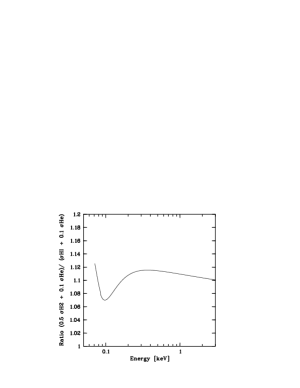
Figure 7: Ratio of photoabsorption cross sections $(0.5\sigma H_{2}+0.1\sigma He)/(\sigma\hbox{H\,{\sc i}}\ +0.1\sigma He)$ of molecular ($H_{\rm 2}$) and atomic (H i) hydrogen. The description for the photoabsorption cross sections of WAM has been used.

We made use of the description of the cross section of molecular hydrogen and of helium as given in WAM, see also Yan, Sadeghpour, & Dalgarno (1998) and we assume for helium an abundance of 10% of hydrogen. We determined the ratio of the effective cross sections $(0.5\sigma H_{2}+0.1\sigma He)/(\sigma\hbox{H\,{\sc i}}\ +0.1\sigma He)$ which we show in Fig. 7. This ratio is $\sim$1.10 for energies above 0.1 keV. This result means that the effective cross section of molecular hydrogen is about 2.2 times the cross section of atomic hydrogen. If we neglect the contribution of metals to the photoabsorption cross section (this assumption may be valid for the LMC where the metal abundance is by a factor of two lower than in the Galaxy) then we can derive the column of molecular hydrogen from Equ. 16.

- (1) Braun, R., 1991, ApJ 372, 54
- (2) Brinkmann, W., Laurent-Muehleisen, S.A., Voges, W., et al. 2000, A&A 356, 445
- (3) Brüns C., Kerp J., Staveley-Smith L. 2001, in Mapping the Hidden Universe: The Universe Behind the Milky Way - The Universe in HI, eds. Kraan Korteweg R.C. & Henning P.A., (ASP Conf. 218), 349
- (4) Cohen, R.S., Dame, T.M., Garay, D.G., et al. 1988, ApJ 331, L95
- (5) de Boer, K.S., 1991, in IAU Symp. 148 ‘The Magellanic Clouds’, eds. R. Haynes & D. Milne, Kluwer; p. 401
- (6) De Grandi, S., Böhringer H., Guzzo L., et al. 1999, ApJ 514, 148
- (7) Falgarone, E., Phillips, T.G., & Walker, C.K. 1991, ApJ 378, 186
- (8) Giacconi, R., Rosati, P., Tozzi, P., et al. 2001, ApJ 551, 624
- (9) Gilli, R., Risaliti, G., & Salvati, M. 1999, A&A 347, 424 [GRS99]
- (10) Gilli, R., Salvati, M., & Hasinger, G. 2001, A&A 366, 407 [GSH01]
- (11) Giuricin, G., Marinoni, C., Ceriani, L., & Armando, P. 2000, ApJ 543, 178
- (12) Haberl, F., & Pietsch, W. 1999, A&A 139, 277 [HP99]
- (13) Hasinger, G., Burg, R., Giacconi, R., et al. 1993, A&A 275, 1
- (14) Hasinger, G., Burg, R., Giacconi, R., et al. 1998, A&A 329, 482 [HBG98]
- (15) Hasinger, G., Altieri, B., Arnaud, M., et al. 2001, A&A 365, 45
- (16) Israel E.P., 1997, A&A 328, 471
- (17) Kahabka, P., de Boer, K.S., & Brüns, C. 2001, A&A 371, 816 (Paper I)
- (18) Kahabka, P., 2001, A&A (subm., Paper II)
- (19) Kim, S., Staveley-Smith, L., Dopita, M.A., et al. 1998, ApJ 503, 674
- (20) Kim, S., Dopita, M.A., Staveley-Smith, L., & Bessell M.S. 1999, AJ 118, 2797
- (21) Lehmann I., Hasinger G., Schmidt M., et al. 2001, A&A 371, 833
- (22) Miyaji, T., Hasinger, G., & Schmidt, M. 2000, A&A 353, 25
- (23) Mizuno, N., Yamaguchi, R., Mizuno, A., et al. 2001, PASJ 53, 971
- (24) Morrison, R., & McCammon, D. 1983, ApJ 270, 119 [MM]
- (25) Richter, P. 2000, A&A 359, 1111
- (26) Rosati P., Della Ceca R., Burg R., et al., 1995, ApJ 445, L11
- (27) Rubio, M. 1999, in New views of the Magellanic Clouds, eds. Y.-H. Chu et al., p.67
- (28) Russell, S.C, & Dopita, M.A., 1992, ApJ 384, 508
- (29) Savage, B.D., Bohlin R.C., Drake, J.F., & Budich, W. 1977, ApJ 216, 291
- (30) Schmidt, M., Hasinger, G., Gunn, J., et al. 1998, A&A 329, 495
- (31) Stanimirovic, S., Staveley-Smith, L., Dickey, J.M., et al. 1999, MNRAS 302, 417
- (32) Stanimirovic, S. 2000, astro-ph/0008327
- (33) Supper, R., Hasinger, G., Lewin W.H.G., et al., 2001, A&A 373, 63
- (34) Tumlinson, J., Shull, J.M., Rachford B.L., et al., 2001, ApJ (in press)
- (35) Wilms, J., Allen, A., & McCray, R. 2000, ApJ 542, 914 [WAM]
- (36) Yamaguchi, R., Mizuno, N., Onishi, T., et al., 2001, ApJ 553, L185
- (37) Yan, M., Sadeghpour, H.R., & Dalgarno, A. 1998, ApJ 496, 1044 [WAM]