Stellar Archaeology: a Keck Pilot Program on Extremely Metal-Poor Stars From the Hamburg/ESO Survey. II. Abundance Analysis

Abstract

We present a detailed abundance analysis of eight stars selected as extremely metal-poor candidates from the Hamburg/ESO Survey (HES). For comparison, we have also analysed three extremely metal-poor candidates from the HK survey, and three additional bright metal-poor stars. With this work, we have doubled the number of extremely metal-poor stars ([Fe/H] $\leq 3.0$) with high-precision abundance analyses. Based on this analysis, our sample of extremely metal-poor candidates from the Hamburg/ESO survey contains three stars with [Fe/H] $\leq-3.0$, three more with [Fe/H] $\leq-2.8$, and two stars that are only slightly more metal rich. Thus, the chain of procedures that led to the selection of these stars from the HES successfully provides a high fraction of extremely metal-poor stars.

We verify that our choices for stellar parameters, derived in Paper I, and independent of the high-dispersion spectroscopic analysis, lead to acceptable ionization and excitation balances for Fe. Substantial non-LTE effects in Fe appear to be ruled out by the above agreement, even at these extremely low metallicities.

For the $\alpha-$elements Mg, Si, Ca, Ti, the light element Al, the iron-peak elements Sc, Cr, Mn, and the neutron-capture elements Sr and Ba, we find trends in abundance ratios [X/Fe] similar to those found by previous investigations. These trends appear to be identical for giants and for dwarfs. However, the scatter in most of these ratios, even at [Fe/H] $\leq-3.0$ dex, is surprisingly small. Only Sr and Ba, among the elements we examined, show scatter larger than the expected errors. Future work (the 0Z project) will provide much stronger constraints on the scatter (or lack thereof) in elemental abundances for a substantially greater number of stars.

We discuss the implications of these results for the early chemical evolution of the Galaxy, including such issues as the number of contributing SN, and the sizes of typical protogalactic fragments in which they were born.

In addition, we have identified a very metal-poor star in our sample that appears to represent the result of the s-process chain, operating in a very metal-poor environment, and exhibiting extremely enhanced C, Ba, and Pb, and somewhat enhanced Sr.

1 INTRODUCTION

Stellar archaeology is the study of present stellar generations in order to infer the characteristics of a previous stellar generation that no longer exists. This is one of the primary aims for investigations of the chemical composition of extremely metal-poor Population II stars, as they provide important clues to the properties (e.g., mass, composition) of the very first objects formed in the Galaxy, the so-called Population III stars.

Long-lived, slowly evolving main-sequence dwarfs are quite suitable for this purpose, since they retain in their atmospheres the elements produced by previously born massive stars that exploded as Type-II supernovae (SN). Unlike the stars presently in the giant-branch stage of evolution, main- sequence stars are expected to be unaffected by internal mixing during their lifetime (although, in some cases, they may exhibit the spectral signatures of contamination from material transfered from close, evolved, companions).

Here we adopt the definition given in Cohen et al. (2001; hereafter Paper I), and we consider only stars with [Fe/H] $\leq-3$ to be extremely metal poor (hereafter EMP).

This definition seems almost straightforward, since all previous investigations (see the review by McWilliam 1997) revealed that at [Fe/H] = $-2.4$ many elemental ratios [X/Fe] (where X is Ba, Sr, Cr, Al, or Mn) display a sudden change in the slope of the relationship of [X/Fe] versus [Fe/H]. McWilliam et al. (1995; hereafter McW95), and others since, have suggested that the patterns observed at very low metallicity can be explained by assuming that a stochastic mechanism is at work, with only a few supernovae responsible for the observed enrichment patterns. By selecting those stars with [Fe/H] $\leq-3$ we can be certain that we are sampling a regime where stars were polluted by the very first supernovae, in an environment likely to have been rather different from that in which the bulk of Galactic stars formed.

The literature concerning EMP stars is continously increasing, as ever more efficient spectrographs at large telescopes come on-line, analysis techniques are refined, and laboratory measurements of fundamental atomic parameters required for detailed abundance analyses are carried out. Interest in this area of astrophysics arises for a number of reasons, since the study of these objects provides insights into such relevant issues as the early chemical evolution of the Galaxy, nucleosynthesis by zero-metallicity massive stars, and the role of the r-process and the s-process in building up the presently observed abundances of neutron-capture elements in stars. Theories of the nucleosynthesis mechanisms themselves benefit from direct comparison with observed abundance ratios in EMP stars, in order to tune model yields. On the other hand, by use of the predicted yields from SN of different masses, one might attempt to decode the observed run of abundances as a function of metallicity, in order to derive the range of numbers and masses of SN contributing to the chemical enrichment in various environments, as well as the epochs of the building up of the Galactic elements (see, e.g., Karlsson & Gustafsson 2001).

Moreover, a direct link to the distant Universe is provided by dating methods that use cosmo-chronology (age estimates based on the radioactive decay of unstable heavy nuclei in EMP stars) to provide independent measurements of the ages of the oldest stars in our Galaxy (Sneden et al. 2000, Cayrel et al. 2001a,b, Toenjes et al. 2001), which can be compared to the ages of other apparently primordial objects such as globular clusters, derived by different methods (see Carretta et al. 2000 and references therein).

The shortcoming, up to now, has been the small size of available stellar samples, due to the relative rarity of EMP stars, their faint apparent magnitudes, and the need for high-resolution, high signal-to-noise (hereafter, S/N) spectroscopy to derive their elemental abundances with suitable precision. The presently available sample of such stars is simply too small for statistical studies that might provide strong constraints on the above-mentioned problems. In fact, summing up all previous high-dispersion analyses of very metal-poor stars (those with [Fe/H] $\leq-2.0$), the total sample with published detailed analyses hardly reaches 50 objects.

We are mainly interested in studying the mechanisms involved in the early chemical evolution of the Galaxy. The large intrinsic spread in (some) elemental ratios found at extremely low metallicities requires a very large database, not only to properly sample the observed trends, but more importantly, to quantify the scatter in the observed elemental abundance distributions as a function of declining metallicity. An increase of available sample sizes for EMP stars by an order of magnitude is required to fully understand the nature of the very first generations of Galactic stars.

In our ongoing study, we intend to exploit the recently completed Hamburg/ESO Survey (HES; Wisotzki et al. 1996, Christlieb et al. 2001a,b) to significantly increase the number of EMP candidates with available high S/N, high-dispersion spectroscopy. Herein we present the results of the Keck Pilot Program on EMP stars, in which we test the ability of the HES to deliver a large sample of newly identified EMP stars for abundance analysis.

The selection, observations, and data reduction of the present sample are discussed at length in Paper I; the present paper will deal only with the abundance analysis. In §2 there is a brief summary of relevant information given in Paper I. The equivalent width measurements and tests of their quality are described in §3. The derived abundances are presented in §4, and discussed in §5. The last section summarizes our present results.

2 OBSERVATIONS, DATA REDUCTION, AND ATMOSPHERIC PARAMETERS

The selection, observational details, and the preliminary data reduction of our program stars are discussed in Paper I. Here we briefly summarize the essential information.

Eight candidate EMP stars from the HES were observed with the HIRES spectrograph (Vogt et al. 1994) at Keck I on two nights in Semptember 2000. On the same nights we also acquired spectra for three EMP candidates from the HK survey (Beers, Preston & Shectman 1985, 1992), as well as three well-studied bright metal-poor stars as comparisons. One of the HES stars turned out to be a re-discovery of a star from the HK survey (HE 2344$-$2800 = CS 22966-045). The relevant parameters of the observations, as well as photometry and the adopted data analysis for all stars in our sample are given in Table 1 of Paper I.

A spectral resolving power of $R=45,000$ was used with an 0.86 arcsec slit projecting to 3 pixels in the HIRES focal plane CCD detector, resulting in spectra covering the region from 3870 to 5400 Å, with essentially no gaps. The figure of merit, F, as defined by Norris, Ryan & Beers (2001; NRB2001), is $\sim 600$ for the worst of our spectra, which guarantees the high quality of our observational material. In this paper, we have doubled the sample of high precision (F $>600$) spectra available for stars with [Fe/H] $<-3.0$, including three newly discovered EMP stars.

Some examples of the spectra are shown in Paper I.

2.1 Adopted Atmospheric Parameters

The procedure used to derive $T_{\mbox{\scriptsize eff}}$ estimates for our program stars is fully explained in §4-6 of Paper I. Very briefly, $T_{\mbox{\scriptsize eff}}$ is derived from broad-band colors, taking the mean estimates deduced from the de-reddened $V-K$ and $V-J$ colors. We used the grid of predicted broad-band colors and bolometric corrections of Houdashelt, Bell & Sweigart (2000), based on the MARCS stellar atmosphere code (Gustafsson et al. 1975), and corrected the colors for reddening by adoption of the extinction maps of Schlegel, Finkbeiner & Davis (1998) (see Table 1 in Paper I).

With $T_{\mbox{\scriptsize eff}}$ fixed, the gravity log($g$) was obtained using the Y² isochrones (Yi et al. 2001); we adopted the 14 Gyr, [Fe/H] = $-3.3$ isochrone. For the star HD 140283 we adopted the log($g$) obtained by Korn & Gehren (2000), derived from the Hipparcos parallax.

Holding $T_{\mbox{\scriptsize eff}}$ and log($g$) fixed, the final overall metallicities [A/H] for the stars were obtained iteratively, by matching observed equivalent widths (EWs) with the synthetic ones computed by integrating the equation of transport at different wavelenghts along each line for the flux, extracted from a model atmosphere in the grid of Kurucz (1995), with no overshooting. In fact, Castelli, Gratton & Kurucz (1997) noted that Kurucz models with the convective overshooting option switched off better reproduce observables in stars other than the Sun. Microturbulent velocities $v_{t}$ were derived by eliminating any trend in derived abundances of Fe I lines with the expected EWs (see Magain 1984).

The adopted atmospheric parameters are summarized in Table 1.

3 EQUIVALENT WIDTHS

Equivalent widths were measured from the one-dimensional, normalized spectra using an automatic routine that determines a local continuum level for each line by an iterative clipping procedure. A fraction $C$ of the 200 spectral pixels centered on the line to be measured is used; the highest 200$C$ pixels are the initial dataset for this process. After various tests, we adopted $C=1$ for the spectra of all stars, except the three very bright stars and the two giants from the HK survey. For these stars $C=0.5$ was used.

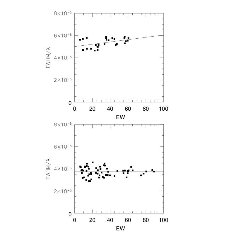
Figure 1: The fiducial relation between the FWHM of lines and their EWs is shown for stars HE 0024$-$2523 (upper panel) and HE 0130$-$2303 (lower panel).

The lines were then measured by a Gaussian fitting routine using a small spectral region (of width 1.6 times the FWHM) centered on their expected location, based on a preliminary determination of the geocentric radial velocity. A number of lines were discarded at this point based on several criteria (features that were not well centered, that were either too broad or too narrow, etc.). After this first measurement, a relation was set between equivalent width and FWHM for each spectrum, examples of which are shown in Figure 1. This relation was then used to obtain a better determination for each absorption line, invoking a different Gaussian fitting routine. This second routine has only one free parameter for each line, effectively the central depth of the line profile, because the line center location is fixed by the average radial velocity determined from all the lines measured in the second step. Again, several criteria were used to discard lines at this point in the analysis (e.g., asymmetric error distributions, indicating lines that are not well centered; large residuals compared with expected noise, etc.). These procedures allow us to obtain very stable measures of the EWs, with random errors close to those expected from photon-noise statistics (Cayrel 1989). Of course, systematic errors may still be present, in particular those related to the adopted reference continua and the relation between equivalent width and FWHM.

Table 2 and Table 3 list the final values of the EWs, along with the adopted atomic parameters for all lines in our list. Table 8 in the Appendix summarizes the comparison between our adopted $gf$’s and the compilation in the NIST database.

In order to evaluate the internal errors in our measurement of EWs, we compare values obtained for two stars in our sample with similar physical parameters. We performed this comparison using two dwarfs (HE 0130$-$2303 with $T_{\mbox{\scriptsize eff}}$, log($g$) , [Fe/H], $v_{t}$ = 6560/4.3/$-$2.96/1.39, and HE 0148$-$2611 with $T_{\mbox{\scriptsize eff}}$, log($g$) , [Fe/H], $v_{t}$ = 6550/4.3/$-$3.07/1.25, respectively) and two giants (CS 22950-046: $T_{\mbox{\scriptsize eff}}$, log($g$) , [Fe/H], $v_{t}$ = 4730/1.3/$-$3.30/2.02, and CS 22878-101: $T_{\mbox{\scriptsize eff}}$, log($g$) , [Fe/H], $v_{t}$ = 4775/1.3/$-$3.09/2.01).

For the two dwarfs, the r.m.s. scatter about the regression line between the sets of EWs (see Figure 2, panel (b)) is 4.5 mÅ. If we assume that both sets of EWs have equal errors, we can estimate typical errors of 3.2 mÅ in the EWs. For the giants (Figure 2, panel a), the r.m.s. scatter is 7.9 mÅ, corresponding to an error of 5.6 mÅ in the EWs for each star. In both cases, these errors are in good agreement with the predicted errors obtained from the formulae derived by Cayrel (1989), given the spectral resolution and the S/N characteristics of our data. This confirms the high quality of the spectra and suggests that no extra sources of noise were introduced by the EW extraction procedure.

An external comparison of our derived equivalent widths for stars in our sample can be carried out using the bright, well-studied metal-poor stars, as well as the stars selected from HK survey.

HD 140283 is the star with the largest number of entries in the Cayrel de Strobel et al. (2001) catalog (note that our data for this star are of higher quality than those for our typical program stars). Among the large list of previous analyses of this star we considered three sets of high quality EWs: Zhao & Magain (1990; $R\sim 20,000$; $S/N\sim 100$), Gratton & Sneden (1994; $R\sim 50,000$; $S/N\geq 150$) and Ryan, Norris, & Beers (1996; hereafter RNB96; $R\sim 40,000$; $S/N\sim 45$). The comparison is shown in the three panels of Figure 3, where the one-to-one correspondance lines are also displayed. The linear regression lines are: EW${}_{us}=0.6$ mÅ+ 0.94($\pm 0.01)$EW_ZM90 , with $\sigma=2.2$ Å from 59 lines in common, EW${}_{us}=-1.4$ mÅ + 1.04($\pm 0.01)$EW_GS94, with $\sigma=2.3$ mÅ from 18 lines in common, and EW${}_{us}=1.22$ mÅ + 0.93($\pm 0.01)$EW_RNB96 , with $\sigma=2.3$ mÅ from 74 lines in common. The very small scatter present in these comparisons again agrees well with the theoretically predicted errors, and confirms the error estimates given above.

For the two giants from the HK Survey in common with the McW95 sample, the linear regression between our measurements and their EWs is EW${}_{McW95}=1.6$ mÅ + 1.04($\pm 0.03)$EW_us, with $\sigma=12.0$ mÅ from 153 lines in the two stars. The McW95 EWs are on average larger than ours (the average offset is 4.1 mÅ); the difference increases for stronger lines. The rather large scatter is most likely due to their measurement errors, arising from spectra having a lower resolving power (R$\sim$ 22,000) and a lower average S/N (typically $30$–$40$) than ours.

4 ABUNDANCE ANALYSIS

Model atmospheres with appropriate parameters (see Table 1) were extracted from the grid of Kurucz (1995) with the overshooting option switched off, interpolating among the nearest models in the Kurucz grid. The abundance analysis was performed using measured EWs (Table 2 and Table 3); the resulting abundances and element ratios for each species in each star are listed in Table 4 and Table 5, and are discussed below . In these tables n is the number of lines used in the analysis of a given ion, and $\sigma$ is the r.m.s. scatter in abundance from individual lines for the set of lines used for a particular ion.

The abundances of neutral species are computed with respect to Fe I, while singly ionized species are compared to Fe II abundances to decrease uncertainties due to the choice of atmospheric parameters.

Table 6 shows how the choice of a given set of atmospheric parameters might affect the derived abundances. Values in this table are computed by varying, one at a time, the individual atmospheric parameters and comparing the resulting abundances with the original values. The amount of the variation is set by the uncertainties established for each of the parameters. This exercise was carried out for a giant (CS 22950-046) and for a dwarf (HE 2344$-$2800), in order to span the whole range of $T_{\mbox{\scriptsize eff}}$ sampled by program stars. In each case, the first four columns show the sensitivity of abundance ratios to changes in each adopted parameter.

The last column of Table 6 lists for each star the sums (in quadrature) of contributions due to the individual parameters; this provides an estimate of the overall uncertainty in abundance for each species arising from errors in the adopted atmospheric parameters. From Paper I we derive estimates of our internal errors of about $\pm 100$ K and $\pm 0.2-0.3$ dex for $T_{\mbox{\scriptsize eff}}$ and for log($g$) respectively. In evaluating the total errors, we took into account the correlation between the error in $T_{\mbox{\scriptsize eff}}$ and the error in log($g$) for each star which arises due to the procedure we adopt to derive surface gravities.

Internal errors in the microturbulent velocity can be checked by using the errors of the relationship between the abundances of Fe I and the expected line strengths. Given the rather large number of measured Fe I lines and the wide range spanned by their intensities, the internal uncertainties in $v_{t}$ are quite small ($\pm 0.12$ km/s), so that the 0.2 km/s adopted in Table 6 can be viewed as a conservative estimate. Unlike abundance analyses of solar metallicity stars in this range of $T_{\mbox{\scriptsize eff}}$, in these very metal-poor stars the term arising from uncertainties in the microturbulent velocity ($v_{t}$) does not dominate the abundance errors due to the general overall weakness of the lines (save for a few isolated specific cases such as the Mg b and Sr II lines).

In the remaining part of this Section we discuss some relevant features of our analysis.

4.1 Iron

Iron abundances for our program stars are summarized in Table 4. There were no credible detections of any Fe II lines in the spectrum of one dwarf (HE 0218$-$2738) from the HES sample.

As we will see in the next subsection, the scatter in the differences between abundances derived from Fe I and by Fe II lines is quite small; we then feel justified in assuming a constant offset between the Fe II and Fe I abundances of stars in our sample in order to obtain a value for the [Fe II/H] ratio for the one star with no measured Fe II lines (HE 0218$-$2738). For this star only, we set $\mbox{Fe~{}II}-\mbox{Fe~{}I}=-0.06$ dex. Abundance ratios of singly ionized species for this star given in Table 4 and Table 5 are then referred to the abundance of Fe II obtained in this way.

According to the strict definition given in Paper I, six stars in the sample can be considered true EMP stars ([Fe/H]$<-3$): the two giants from the HK survey, and four dwarfs from the HES sample. Two other stars, BS 17447-029 and HE 0130$-$2303, are borderline, following this definition.

4.1.1 Uncertainties in Fe Abundances

Among the various diagnostics that can be used to test our Fe abundances, we considered the differences between the abundances derived from neutral and singly ionized Fe lines (hereinafter $\Delta$[Fe/H]_II-I), and the slopes of the abundances derived from neutral Fe lines with excitation potential (hereafter, $\Delta(Fe~{}I/\chi)$). (See Figure 4 a,b, where both these quantities, derived for each star, are plotted against effective temperature. Values of these parameters are listed for each stars in the last two columns of Table 1.) These diagnostics are useful because both temperatures and gravities were derived independently of our line data (note however that we adjusted $v_{t}$ in order to reproduce similar abundances from weak and strong lines). Ideally, we expect both $\Delta$[Fe/H]_II-I and $\Delta(Fe~{}I/\chi)$ to be null. However, there are various reasons why this might not occur in practice: (i) the atomic parameters adopted in our line analysis may themselves contain systematic offsets or trends; (ii) our adopted effective temperature scale, or the theoretical isochrone used to derive gravities, may be incorrect; (iii) the 1-d theoretical constant-flux model atmospheres used throughout this paper may be not an adequate representation of the real stellar atmospheres; (iv) departures from LTE in the formation of Fe lines may significantly affect the derived abundances; and (v) observational errors both in the colors (affecting individual temperatures) and in the equivalent widths may introduce significant scatter. We leave aside here other possibilities, such as binarity of some stars, that might be used to explain individual discrepant points.

Clearly the list of possible concerns is long. It is thus not surprising that both $\Delta$[Fe/H]_II-I and $\Delta(Fe~{}I/\chi)$ exhibit definite zero-point offsets, and also possible trends with effective temperature (or, equivalently, luminosity). On average we have $<$$\Delta$[Fe/H]_II-I$>=-0.07$ dex with $\sigma$($\Delta$[Fe/H]_II-I) = 0.11 dex (in the sense that abundances from neutral Fe lines are larger than those obtained from singly ionized Fe lines; the error value is the r.m.s. scatter of the individual values for each star), and $<\Delta(Fe~{}I/\chi)>=-0.046$ dex/eV with $\sigma[\Delta(Fe~{}I/\chi)]=0.025$ dex/eV (where we have excluded HE 0132$-$2429 and HE 0242$-$0732, two stars that show obvious large trends of abundances with line excitation, and which will be discussed later). If we exclude the two giants, the average value of $\Delta$[Fe/H]_II-I becomes $-0.06\pm 0.03$ dex, with a $\sigma=0.11$ dex (11 stars). To quantify these values in terms of uncertainties in the atmospheric parameters, as suggested by the referee, we note that a difference in $\Delta(Fe~{}I/\chi)$ of 0.05 dex/eV corresponds to a temperature difference of $\sim 250$ K, and that a difference of 0.07 dex in the iron abundances derived from Fe I and Fe II implies a difference of about 0.16 dex in log($g$).

When considering the implication of these tests, several points should be taken into account:

• The Fe oscillator strengths we used throughout this paper are the best determinations we found in the literature; they are discussed at length in a number of papers devoted to the solar Fe abundance (see e.g. Asplund et al. 2000, and references therein). The transition probabilities for the Fe I lines were used as published, in spite of the fact that a small offset may exist between values obtained from the absorption experiments of the Oxford group, and those from the selected laser induced excitation experiments by the Hannover group. (A line-to-line comparison shows that these latter values are larger on average by $\sim 0.03$ dex.) Furthermore, the zero point of Fe II oscillator strengths is not yet firmly established, and possible offsets of several hundredths of a dex are easily possible (see the discussion in Asplund et al. 2000).

• Even using the best available oscillator strengths, small offsets in the abundances are present also in a solar analysis done following precepts similar to those adopted for the program stars (LTE, 1-d model atmospheres from the Kurucz CD-ROMs, etc.) and $EW$s from Rutten and Van der Zalm (1984). In this case we find Fe abundances of $\log n(Fe)=7.512\pm 0.012$ (with an r.m.s. scatter of 0.069 dex for individual lines) from 34 Fe I lines, and $7.450\pm 0.016$ (r.m.s. scatter of 0.085 dex) from 27 Fe II lines (only lines with $EW<100$ mÅ were considered, to reduce concerns related to the handling of collisional damping). In view of the roughness of the methods used, these abundances compare quite well with the much more sophisticated results obtained by most recent analyses of the solar photospheric spectrum (e.g., Asplund et al. 2000). Our solar analysis yields $<\Delta(Fe~{}I/\chi)>=-0.023$ dex/ev with $\sigma(\Delta(Fe~{}I/\chi))=0.009$ dex/eV, which is quite similar to the value we obtain for our very metal-poor program stars. Note, however, that the set of lines used in this solar analysis is disjoint from that used for the stellar analyses, because those lines measurable in extremely metal-poor stars are heavily saturated in the solar spectrum. Line selection is of particular importance for the determination of $\Delta(Fe~{}I/\chi)$, which is also sensitive to the value adopted for the microturbulent velocity. On the other hand, trends of abundances with line excitation have been found also in previous, much more accurate analyses of the solar photospheric spectrum (see e.g. Grevesse & Sauval 1999). In this respect, it is interesting to note that such a trend is not present when 3-d models are used to analyse Fe lines in the solar spectrum (Asplund et al. 2000). 3-d effects may be expected to have an even larger impact on the analysis of metal-poor stars than in the case of the Sun (see Asplund et al. 1999). In fact, due to the lower opacity in the atmospheres, the lines are expected to form deeper in the stars, where the impact of convection is larger, and possibly the granulation contrast larger as well.

• The r.m.s. scatter of the individual values of $\Delta$[Fe/H]_II-I (0.11 dex) roughly agrees with the expected uncertainties. To show this, we assumed that the internal errors in $T_{\mbox{\scriptsize eff}}$ are those estimated in Paper I, i.e. $\pm 75$ K, possibly increasing up to $\pm 150$ K for turnoff stars only. To estimate the corresponding errors in log($g$), one needs the slope of the isochrone in the region of interest, namely $\Delta$(log($g$)/$T_{\mbox{\scriptsize eff}}$) = $\sim$0.003 dex/K along the RGB and much less ($\sim$0.0005 dex/K) for less-evolved evolutionary stages (subgiants and dwarfs). Below the main-sequence turnoff the slope reverses in sign. Reading from Table 6 the changes in Fe I and Fe II abundances expected for a 100 K increase in $T_{\mbox{\scriptsize eff}}$ (with consequent changes in log($g$) and overall metallicity [A/H]), the resulting value of $\Delta$[Fe/H]_II-I would be about +0.08 dex for giants and $-0.04/-0.08$ dex for subgiants/dwarfs. When we sum these values in quadrature with the internal error due to uncertainties in the measured EWs, for our Fe II abundances (typically 0.05 dex for giants and 0.09 dex for dwarfs, where only a few lines were usually observed), we find that the observed scatter in the values of $\Delta$[Fe/H]_II-I is reproduced.

• An interesting feature of our analysis is that adoption of a systematically incorrect $T_{\mbox{\scriptsize eff}}$ scale would, as described above, yield values of $\Delta$[Fe/H]_II-I of opposite signs for dwarfs and giants when the resulting changes in log($g$) are included. However, a larger sample is probably needed to explore this possibility. Again, adoption of realistic 3-d model atmospheres for the program stars might provide better insight into this issue (Asplund et al. 1999).

For most of the sample stars, the general trends shown in Figure 4 can probably be explained by $T_{\mbox{\scriptsize eff}}$ scale errors or model atmosphere uncertainties. However, two stars (HE 0132$-$2429 and HE 0242$-$0732) display trends of abundance with excitation potential ($\Delta(Fe~{}I/\chi)\leq-0.15$) that are much larger than can be induced by typical errors in the stellar parameters, primarily in the $T_{\mbox{\scriptsize eff}}$. The trend found for HE 0132$-$2429 is clearly significant, and does not depend on inclusion or not of one or two lines (see Figure 5). The situation for HE 0242$-$0732 was less clear since most of the apparent trend obtained when the atmospheric parameters of Paper I were used for this star was due to a single line.

In order to remove these trends, $T_{\mbox{\scriptsize eff}}$’s much lower (by $\sim 500$ K) than those given by the colors would be required. Such differences cannot be due to the reddening corrections, because these are too small. Furthermore, $T_{\mbox{\scriptsize eff}}$’s derived from the H_δ profiles support the high $T_{\mbox{\scriptsize eff}}$ values given by colors (see Paper I: however, we note that H_δ is quite weak for HE 0132$-$2429, so that precise determination of $T_{\mbox{\scriptsize eff}}$ is not easy for this star). Also, it does not seem possible to invoke contamination by a bluer companion such as main-sequence turnoff star (this explanation may obviously only be considered for HE 0132$-$2429). To demonstrate this, we note that the observed (de-reddened) $V-K$ color for this star is $V-K=1.86$. This color can be obtained by combining the flux from a star along the RGB (with $M_{V}=1.4$, $V-K=1.91$) and a star at the main-sequence turnoff ($M_{V}=3.8$, $V-K=1.05$). In the (observed) blue part of the spectrum, the secondary would be about 7 times less luminous than the primary: it would be difficult to detect such a star if the radial velocity difference were small. However, the difference between the color of the primary and that of the whole system would be only 0.05 mag in $V-K$, corresponding to less than 100 K in $T_{\mbox{\scriptsize eff}}$. This difference is far too small to explain the trend of Figure 5.

In the case of HE 0242$-$0732, the automatic EW measuring routine did not pick up any Fe II lines. Hence we measured the EWs of the four strongest Fe II lines expected to be present in our spectra, at 4233.16, 4923.93, 5018.45 and 5169.03 Å, by hand. All these lines are only a bit stronger than noise, so that their EWs are somewhat uncertain; however, they surely are not much stronger than our estimates. Using these lines, a lower limit for the surface gravity may be obtained by assuming that log n(Fe I) $\sim$ log n(Fe II).However, the Fe II lines in this star are clearly much weaker than expected on the basis of the atmospheric parameters used thus far ($T_{\mbox{\scriptsize eff}}$=6455, log($g$)=4.2) from Paper I. This forced us to consider both a lower temperature, and a less evolved evolutionary phase for this star. A lower temperature is also suggested by the H_δ profile.

In Paper I we already noticed that the $K$ magnitude for this star from the 2MASS is quite uncertain (it is the faintest star in the infrared in our sample). On the whole, it might be reasonable to disregard for this star $T_{\mbox{\scriptsize eff}}$ from $V-K$, and use only the temperature from the more accurate $V-J$ color, that is to adopt a $T_{\mbox{\scriptsize eff}}$ of 6360 K. Also, it may be reasonable to consider a gravity consistent with a MS star at this $T_{\mbox{\scriptsize eff}}$ (log($g$)=4.4), rather than a star brighter than the turn-off.

We then repeated the analysis with the revised stellar parameters, after adding manual measurements of four more weak Fe I lines, to extend the range of excitation potential sampled. With the same procedure adopted above, we derive the full set of parameters for HE 0242$-$0732 of 6360/4.4/$-$3.21/0.40. The abundance from Fe II lines is still lower than that obtained from Fe I lines, although the difference is roughly halved with these parameters with respect to the original discrepancy). We regard this new analysis as quite robust, and we adopt these new parameters for this star.

Using these new parameters and the slightly more extended line list, the discrepancy of star HE 0242$-$0732 in Figure 4 is reduced. There is still a trend of abundances with E.P., but it is well within the error bars, which are large, due to the small range in E.P. of available Fe I lines. The trend is not very different from the trends shown by the other stars in the sample. Another improvement achieved using this set of atmospheric parameters is that the Ti II abundance (that was previously the lowest in the sample) now is raised to +0.25 dex, and does not stand out anymore as outlier in Figure 7 (see below).

4.1.2 Comparison with results from a purely spectroscopic analysis

As a further check of our adopted procedure to derive atmospheric parameters, we performed a purely spectroscopic analysis, deriving temperatures, surface gravities, overall metal abundance and microturbulent velocities from the equivalent widths alone. In this process, we ignored the photometry that forms the basis of the assignment of stellar parameters used in Paper I.

We adopted HE 0242$-$0732 as typical of our program stars (it is neither the best nor the worst case, as far as the quality of observational material is concerned); however it does represent an extreme case of differences between results of our original analysis (with temperatures based on colours, and gravities from the color-magnitude diagram), and those from a purely spectroscopic analysis. The spectroscopic set of parameters in this case is: an effective temperature $T_{\mbox{\scriptsize eff}}$=5250 K (obtained by zeroing the slope in the relation of Fe abundances with the excitation potential of lines), a surface gravity log($g$)= 2.55 (assuming that Fe I and Fe II lines must give the same iron abundance), [A/H]$=-4.21$ (given by the abundance of iron) and a microturbulent velocity of 0.45 km/sec (derived eliminating trends of abundances with expected line strength for Fe I lines).

This set of parameters is quite different from that of our original analysis. To estimate the appropriate error bars, we must take into account the covariance among the errors, and hence we performed the following exercise. Using this set as a starting point, we used the same set of Fe lines to repeat the analysis changing the $v_{t}$ value until the 1$\sigma$ value from the slope of the abundance/line strength relation was reached, and optimizing at the same time the other parameters at their best value. The resulting set ($T_{\mbox{\scriptsize eff}}$, log($g$), [A/H], $v_{t}$), was: 5480/2.85/-4.07/0.74. Starting then from this second set of parameters, we changed the effective temperature in order to have all parameters optimized when the 1$\sigma$ value from the starting slope of abundances vs E.P. relation was reached (still leaving the trend of abundances with expected line strength off by 1 $\sigma$ from its best value). In this way we get a third set of parameters: 5760/3.45/-3.81/0.78. Finally, we repeated the same exercise, but now achieving a change of 1$\sigma$ in the difference between Fe I and Fe II (again, leaving trends of abundances with expected line strength and excitation off from their best value by 1 $\sigma$): the resulting final set of parameters was 5780/3.05/-3.79/0.88.

We emphasize here that this last set of parameters is still statistically acceptable: each of the residual trends is not larger than its 1$\sigma$ r.m.s. error.

A simple comparison between this last set and our starting point allows us to give an estimate of 1$\sigma$ internal errors associated with a purely spectroscopic analysis; we consider these values more appropriate than those derived from considering each individual parameter as independent from the other. Uncertainties are: $\pm 530$ K in $T_{\mbox{\scriptsize eff}}$, $\pm 0.43$ km/s in $v_{t}$ and $\pm 1.3$ dex in log($g$). On the whole, the uncertainty in the overall metal abundance from the purely spectroscopic analysis is $\pm 0.42$ dex! This very large error bar is more than twice that deduced by assuming that the atmospheric parameters are independent each other. This is mainly due to the correlation existing between excitation potential and line strength for Fe I lines. We conclude that the intrinsic uncertainties in a purely spectroscopic approach are too large to secure a robust result when dealing with extremely metal poor stars, where the number of reliable lines measured is rather small, particularly for Fe II, uncertainties in the EWs of individual lines are not negligible, and the range in excitation potential is limited.

For these reasons, we think that the procedure we have adopted that fixes temperature and gravity by independent means works better in our case. The previous exercise, for example, shows that using only information provided by Fe lines (as it is done in the purely spectroscopic analysis), we could not say if HE 0242$-$0732 is an RGB or HB star (5250/2.55), or a subgiant (5780/3.05). Note that both these combinations of $T_{\mbox{\scriptsize eff}}$ and log($g$) are compatible with the same isochrone, and would then appear as plausible solutions.

4.1.3 Checks on Departures from LTE for Fe

Having derived gravities from $T_{\mbox{\scriptsize eff}}$ and isochrones only, we can in principle use the ionization balance of Fe in order to check if Fe abundances are affected by departures from Local Thermodynamic Equilibrium (LTE). This issue is the subject of considerable debate, since Thevenin & Idiart (1999) suggested that LTE analyses tend to underestimate the Fe I abundances (by a few tenths of a dex in extremely metal-poor stars), while Gratton et al. (1999) pointed out that large ($>0.2$ dex) departures from LTE are unlikely, and LTE should instead be a very good assumption for Fe line formation in metal-poor dwarfs. In view of the large uncertainties still present in the collisional cross sections (e.g., Gehren et al. 2000), and given the limitations in the adopted model atoms, there is no way at present to decide from first principles which of these analyses is valid.

There is no evidence in our data for a large Fe overionization, judging from the upper panel in Figure 4. As discussed above, the average difference in abundances from Fe I and Fe II lines is only marginally different from zero. Moreover, almost all stars show differences which have the wrong sign for overionization. This seems to rule out large departures from LTE in the formation of Fe lines in metal-poor stars.

On the other hand, the discussion of §4.1.1 showed that there are so many possible uncertainties still remaining in the temperature scale, in the model atmospheres, and in the oscillator strengths, that small NLTE effects (at a level of 0.1 to 0.2 dex) cannot be firmly excluded from our data.

4.2 The $\alpha-$elements

We detected lines arising from two stages of ionization for titanium, hence we can use the ionization equilibrium of this element as an additional clue for the presence of NLTE effects. In fact, given the lower ionization potential of Ti I, it may be expected that this element ought to be even more vulnerable to non-LTE effects than is iron. There is no conclusive evidence for departure from LTE from the Ti I/Ti II abundance. From the data in Table 5, a trend for decreasing Ti II $-$ Ti I differences as $T_{\mbox{\scriptsize eff}}$ increases seems to be present, with the two giants showing somewhat larger (positive, i.e., abundances from Ti II larger than those from neutral Ti) differences. However, even in this case we believe that the safest approach is not to draw any firm conclusions until a larger sample becomes available. We are concerned that there is a possible bias resulting from the rather uncertain Ti I abundances in the warm, metal-poor dwarfs that are clustered around Ti II$-$Ti I $\sim-0.2$ to $-0.3$ dex. Moreover, we are not aware of any computations of NLTE effects for Titanium.

We note in passing that data from McW95, and the few stars from RNB96 with both Ti I and Ti II measured (all giant/subgiant stars) show the same pattern of differences in titanium abundances as a function of metallicity, with an average value of Ti II$-$Ti I just below zero; values as low as about $-0.3$ dex can be found.

4.3 Aluminum

For Al, the only accessible feature in our HIRES spectra is the resonance doublet at 3944-3961 Å. However, a reliable measurement of these lines is somewhat hampered by the proximity of H_ϵ to the 3961 Å line. Moreover, the line at 3944 Å is disturbed by CH features in some of our stars (Arpigny & Magain 1983).

Apart from these problems, this doublet is not an ideal abundance indicator in view of the presence of possible large departures from LTE, extensively discussed by Baumüller & Gehren (1997). They found that LTE analyses produce a large underestimate of Al abundances; they give NLTE corrections (about 0.6 dex) for the resonance lines in their Table 1.

Very recently, Gratton et al. (2001) found that inclusion of these corrections improves the agreement between Al abundances derived in globular cluster dwarfs from this doublet and from the IR high excitation doublet at 8772.9$-$8773.9 Å, which is believed to be less affected by departures from LTE. This provides further support for the calculations of Baumüller & Gehren. We therefore interpolated Table 1 of Baumüller & Gehren to derive corrections to the Al abundances listed in Table 4.

4.4 The Fe-peak Elements

Apart from Fe, our spectra provide useful information on the abundances of three additional Fe-peak elements (Sc, Cr, and Mn). Lines of the remaining elements are too weak to be reliably measured, due to the combination of low metal abundance and high temperature of most of our stars.

Lines of Sc and Mn exhibit hyperfine structure (hereafter, HFS), mainly due to their non-zero nuclear magnetic moments. HFS is expected to be rather narrow for the Sc II lines, with small impact on abundances, hence we neglect it. On the other hand, Mn lines exhibit broad HFS: this was taken into account using data from Booth et al. (1983).

4.5 The Neutron-Capture Elements

We measured lines for two n-capture elements (Sr and Ba; in both cases we observed the resonance lines of the singly ionized species). The Eu II line at 4129.7 Å is within the observed spectral region, but it is too weak to be detectable in any of our spectra. Note that none of our stars belongs to the group of rare stars that exhibit strong overabundances of elements produced by the r-process, which includes CS 22892-052 and CS 31082-001. The classification of BS 17447$-$029 is somewhat uncertain; this star shows high abundances of Sr and Ba, but does not have detected Eu (nor any strong CH features). This star may be a mildly r-process-enhanced star.

HFS due to both non-zero magnetic moment and isotope splitting is significant for the Ba II line at 4554.04 Å. The HFS corrections were evaluated using the data of Steffen (1985); those recently calculated by McWilliam (1998) are very similar. Note, however, that we do not know the relative abundances of the different Ba isotopes: our assumed distribution is the solar one, and may be inappropriate for metal-poor stars.

5 DISCUSSION

5.1 Results from the Keck Pilot Program

5.1.1 Comparison for Stars in Common with McWilliam et al. (1995)

There are two stars in common between our sample and that analyzed by McWilliam et al. (1995): the two giants CS 22878-101 and CS 22950-046. The adopted $T_{\mbox{\scriptsize eff}}$ are quite similar (ours being larger on average by 38 K); we adopted larger surface gravities (on average by 0.3 dex), and smaller microturbulent velocities (on average by 0.52 km/s). The effects of these differing choices of log($g$) and of $v_{t}$ are in most cases similar in magnitude but of opposite sign, and so somewhat cancel out. The differences between our and the McW95 analysis are as follows (in the sense ours-McW95; in parenthesis we give the difference expected from the atmospheric parameters): Fe +0.09 (0.13); Mg +0.15 ($-$0.09); Al $-$0.17 (0.11); Si +0.04 ($-$0.07); Ca $-0.15(-0.09$), Sc +0.17 (0.07); Ti I $-0.24(-0.09$); Ti II $-$0.04 (0.06); Cr +0.02 (0.01); Mn $-0.19(0.14)$; Sr +0.20 (0.24); Ba $-0.30(+0.02)$.

In several cases there is a reasonable agreement between the observed and expected offsets. The large difference for Mg is due to the $gf$’s we adopted; see the Appendix. The differences for Al and Si are discussed elsewhere in the text. Part of the difference for Sc is due to the fact that we neglected the HFS for this element (while it is considered by McW95).

5.1.2 $\alpha-$elements

Abundances for the $\alpha-$elements are summarized in Table 4 and Table 5, and shown in the left-hand panels of Figure 6 and Figure 7. We also show, for purpose of comparison, the results from the literature of previous high-dispersion studies: McWilliam et al. (1995) for a sample of 33 metal-poor giants, and a compilation of literature data taken from NRB2001. In addition to the five EMP giants they studied, NRB2001 used high-quality data compiled from the literature to discuss the chemical evolution of the Galaxy. In the construction of Figures 5–9, 11, 12 and of Table 7 we employ three datasets from that paper: (i) the data from the Ryan/Norris/Beers group (collectively RNB hereafter): Ryan, Norris & Bessell (1991); Ryan, Norris & Beers (1996); Norris, Beers & Ryan (2000); NRB2001; (ii) the data from Gratton/Sneden (hereafter GS): Gratton (1989); Gratton & Sneden (1987, 1988, 1991, 1994); and (iii) Stephens (1999).

Following Table 1 in NRB2001, data from McW95 come from lower quality spectra, but $\alpha-$elements have strong lines in metal-poor stars, hence concerns due to somewhat lower resolution and S/N are limited in this case. The overall patterns for each of the $\alpha-$elements are quite similar, even though our sample is mostly composed of dwarfs. Unweighted mean values for [Mg/Fe], [Ca/Fe], [Ti/Fe]I and [Ti/Fe]II are respectively 0.31 ($\sigma=0.24$), 0.35 ($\sigma=0.12$), 0.40 ($\sigma=0.19$), 0.36 ($\sigma=0.15$) dex, to be compared with 0.40 ($\sigma=0.22$), 0.44 ($\sigma=0.13$), 0.32 ($\sigma=0.19$) and 0.30 ($\sigma=0.13$) in the McW95 sample.

The average difference in the sense [$\alpha$/Fe]_us $-$ [$\alpha$/Fe]_McW95 is only $-0.01,\sigma=0.08$ dex, suggesting that there is no significant offset in the mean $\alpha-$element abundances between metal-poor dwarfs and giants.

The only apparent offset seems to lie in the Si abundances. However, our [Si/Fe] values are based on only one strong line, Si I 3905 Å, and this line was disregarded by McW95 since it exceeded their adopted reduced equivalent width limit. Unfortunately, all other Si lines in the spectral region sampled by our spectra are vanishingly weak in these warm metal-poor stars. The large scatter in the plot [Si/Fe] vs. [Fe/H] is present in all samples of metal-poor stars, but the observational problems suggest that this could be an artifact of the still uncertain abundance analysis for this ion.

We note that 4 out of 14 stars in our sample exhibit distinctly low [Mg/Fe] ratios, close to the solar ratio. It would be interesting to have more insight into these objects by coupling chemical data with kinematical information. This is deemed important, since more and more stars which show underabundances among the $\alpha$-elements are being discovered by several investigators, e.g., stars with [Fe/H]$<-2$ and [Mg/Fe]$<0.1$ in the upper-left panel of Figure 6. All our low-Mg stars are dwarfs, but they are equally intermingled with giants in other samples. Often, when orbital parameters can be estimated, these objects are seen to have large apogalacticon distances, suggesting their possible origin in lower mass stellar systems with chemical evolution histories that were distinctly different from that of our Galaxy, and were subsequently accreted into our Galaxy (see King 1997; Nissen & Schuster 1997; Carney et al. 1997).

At present we do not have good information about Galactic orbits for all the objects in our sample, but the expected extension of the USNO CCD Astrograph Catalog (Zacharias et al. 2000) from the southern sky to the northern sky, as well as the forthcoming release of proper motions from the GSC-II catalog (and other ongoing proper motion programs) should fill the 6-dimensional parameter space, when coupled to the radial velocity information. We thus defer the study of possible correlations of chemistry and kinematics to future works.

The scatter seen in Ca abundances is similar to the one in McW95 stars, if one disregards the star with [Ca/Fe]$\sim 0.9$ in their sample, and seems to be lower than the scatter observed in the RNB data. Our element ratios [Ca/Fe] seem to be slightly lower, on average, than those from McW95, and more in agreement with data from RNB, even if we do not find stars having very low Ca abundances ([Ca/Fe]$<0.1$). Excluding the four most metal-poor stars in the McW95 sample, the other datasets do not show any trend for Ca abundances increasing for decreasing metal abundances.

5.1.3 Aluminum

The NLTE Al abundances ([Al/Fe]_NLTE) for the program stars are shown in Figure 8 (central panel) as a function of [Fe/H]. Al abundances derived without these corrections are shown in the upper panel of this Figure. In order to make a meaningful comparison, the NLTE corrections from Baumüller & Gehren (1997) were applied as well to the abundances in the samples from the literature, also shown in Figure 8, with the same symbols as in previous Figures.

Our average [Al/Fe] value without correction for NLTE is $-0.59(\sigma=0.15)$ dex, which is not too far from the mean value as defined at [Fe/H]$\sim-3$ by the robust trend computed in RNB96 (their Figure 3c). This means that as far the EWs of these resonance lines are concerned, the agreement between the two different investigations is quite good. Moreover, an offset in the two metallicity scales is not likely to be present, even if we have only one star in common, the well studied HD 140283. We considered for this star the differences in atmospheric parameters $T_{\mbox{\scriptsize eff}}$  log($g$) and $v_{t}$ (5750/3.40/1.40, RNB96; and 5750/3.67/1.10, this study). Reading from Table 3 of RNB96 the changes in [Fe/H] associated with these differences, the metallicity given by RNB96 ([Fe/H]$=-2.54$) would increase by only 0.03 dex. We can say that part of the difference with our value [Fe/H]$=-2.44$ can be explained by differences in the EWs and part ($\sim 0.03$ dex) by a different distribution over excitation potential of the sample of lines used in the analysis.

To compare our results with models of chemical evolution, we adopt, based on theoretical and observational reasons discussed above, the abundances for Al derived with the NLTE corrections included. In this case, our average values [Al/Fe]$=+0.10(\sigma=0.22)$ and [Al/Mg]$=-0.21(\sigma=0.23)$ are not dramatically different from the prediction of models by Timmes et al. (1995).

The case for the sample of McW95 looks quite different. A large scatter in Al abundances is seen among their stars at each metallicity, and the reason is not obvious. We note that all stars in that sample are giants, and the derivation of atmospheric parameters is somewhat more uncertain for giants than for dwarfs.

In conclusion, we have to agree with RNB96 that the higher average [Al/Fe] ratio found by McW95 has no obvious explanation.

5.1.4 The Iron-Peak Elements: Sc, Cr, Mn

Our results for the iron peak elements are shown in the left three panels of Figure 9. In the region $-2<$[Fe/H]$<-1$, the Cr and Mn abundances show a relatively small scatter as is expected when the contributions from many SN events average over the IMF and yields (see Figure 9). On the other hand, below [Fe/H]$\sim-2$ the scatter increases, which is characteristic of stochastic models of chemical enrichment. The correlation in the upper panel (Cr increasing as Mn increases) could be explained either if the production of both elements is a function of the mass cut (since they have slightly different atomic number, they are produced in nearby, yet different regions) or if there is a different neutron excess in this metallicity range.

A deeper insight can be obtained looking at Figure 10, where we plot in the upper panel the ratios [Cr/Fe] vs. the abundance ratios [Mn/Fe] for stars in the collected “big sample”, described in §5.2, with [Fe/H]$<-2$. In this low-metallicity regime we expect to see the classical signature of Type II SN nucleosynthesis. However, since the neutron excess is known to be a function of metallicity, we can test this hypothesis by removing the trend with metal abundance. To this end, we used two linear regressions to fit the [Cr/Fe] and [Mn/Fe] vs. [Fe/H] distributions (for stars with [Fe/H]$<-2$) and computed the residuals of the abundance ratios with respect to these two fits. The residuals are shown in the lower panel of Figure 10.

Again, a correlation is evident for both our program stars and for the stars in other samples from literature. Note that the evidence for a correlation holds even if we disregard the extreme case of HE 2344$-$2800, with its large Mn I abundance. This star has a high-S/N HIRES spectrum and the high [Mn/Fe] ratio in this star is real beyond any doubt: in Figure 11 we compare the spectrum of this star in the region around the Mn lines at 4030-34 Å with the spectrum of HE 0024$-$2523, with very similar atmospheric parameters, but no measurable Mn lines.

What do these findings tell us? Following Heger & Woosley (2001) and Qian & Wasserburg (2001a,b,c), very massive stars (VMS) that belong to the Population III explode as pair-instability supernovae and are expected to produce a [Cr/Fe] ratio approximately constant, while [Mn/Fe] should decrease with metallicity, since nuclei having odd nuclear charge are underproduced by VMS. Therefore, the signature of VMS in the iron-peak elements Cr and Mn should be a lack of correlation. Since we do observe such a correlation, our results point toward a likely scenario discussed e.g. by Nakamura et al. (1999) who explain the trends of [Cr/Fe] and [Mn/Fe] ratios decreasing with decreasing [Fe/H] as due to a variation of mass cuts in type II SN as a function of the progenitor mass. The trends we observe can be reproduced if the mass cut was smaller for the larger mass progenitor that presumably was the first to evolve and pollute the gas in the early halo.

5.1.5 Heavy Elements: The n-capture Elements Sr and Ba

Strontium abundances were derived from the Sr II resonance lines at 4077 Å and 4215 Å, the other accessible lines being vanishingly weak in EMP stars. These strong resonance lines are relatively unaffected by blends in very metal-poor stars and can be easily measured for most of our program stars, excepting those with the lowest S/N values. On the other hand, since these are resonance lines, they are saturated in most stars. Hence, the derived [Sr/Fe] ratios are sensitive to the details of the stellar parameters and of the adopted model atmosphere (see Table 6). In particular, they are affected by uncertainties in the microturbulent velocity. However, since we derive $v_{t}$ values by using a fair number of Fe I lines in each star, this is not a serious issue.

Figure 12 presents our results as compared to data from the literature. In this Figure we plot in the upper panels the run of [Sr/Fe] as a function of the metallicity [Fe/H] for our program stars and a compilation of previous studies: McWilliam et al. (1995) and RNB for very metal-poor dwarfs and giants and Gratton & Sneden (1994; GS94) for somewhat more metal-rich objects. While systematic offsets may be present between different studies (mainly depending on the $T_{\mbox{\scriptsize eff}}$ scale adopted and on the set of model atmospheres), the overall agreement is fairly good.

Our data confirm once more that at metallicities [Fe/H]$\sim-3$ (or below $-2.4$, the point where most heavy element patterns show a change in slope, McW95) there is a huge spread in the observed [Sr/Fe] values, reaching almost 3 dex. This scatter is not linked to a particular evolutionary stage, being present among both dwarf and giant stars. The increase in scatter for [Sr/Fe] values for decreasing metallicity is commonly explained by the classical enrichment of r-process elements from explosions of massive Type II SN (above 12–15 M_⊙) in the framework of a stochastic enrichment mechanism (McW95). In this scenario, if only few supernovae contribute to the production of Sr, we expect a strongly asymmetric distribution in the logarithmic plane [Sr/Fe] vs. [Fe/H], with more stars with low [Sr/Fe] than stars with high Sr.

The r-enhanced region ([Sr/Fe]$>0$ in the upper panels of Figure 12) is attributed to the same classical site of r-process production, but restricted in this case to very few SN less massive than 12–15 M_⊙. As a consequence of the limited number of objects contributing to the enrichment, the whole process has a strongly stochastic behaviour revealed in a few stars with abnormally high r-process abundances.

Ba abundances were derived from the Ba II resonance line at 4554.0 Å. This line has appreciable HFS, taken into account when computing the abundances of Table 5 using data from Steffen (1985). Figure 12 (lower panels) summarizes and compares our results with previous studies. Apart from the few objects above [Ba/Fe]$\sim 1$ (whose origin is somewhat different, see below), Ba shows a decrease for [Fe/H]$<-2$ and less scatter than the lighter n-capture element Sr. The main features of this Figure are commonly explained by the two classical sources of Ba production: the main s-process in intermediate-mass stars (4–7 M_⊙) evolving through the asymptotic giant branch (AGB) phase, plus a contribution by the r-process in SN. As a consequence of the evolutionary stellar timescales involved, what is seen below [Fe/H]$=-2$ is essentially the enrichment of r-elements from massive Type II SN, whose entire evolution from birth to death is much quicker than the timescale required for lower-mass stars to reach the AGB and for complete mixing of the winds from these stars.

Finally, Figure 13 shows the relation between the abundances of Sr and Ba – these elements are often chosen to represent the behavior of light and heavy n-capture elements, respectively. This plot is quite instructive, since we can see that, for the majority of the stars, the [Sr/Fe] and [Ba/Fe] ratios lie almost exactly on a line that is simply that of a scaled solar composition. The low-Sr, low-Ba region reflects the classical r-enrichment by massive SN. However, in this Figure we can also see a sort of branch or plume of stars having a high Sr content, and proportionally less Ba. This group of stars seems to lie outside the general trend. If confirmed, this could imply that a unique site of r-process production might not be not sufficient, and we would require an additional nucleosynthesis mechanism able to provide almost exclusively light n-capture elements (such as Sr) with only a small amount of heavier n-capture elements (like Ba). This idea is not new (Wasserburg & Qian 2000), but it will require a much larger sample of stars, analyzed in a consistent and homogeneous manner, in order to be tested.

5.2 A “Big” Sample

The right panels in Figure 6, Figure 7, Figure 9 and Figure 12, as well as the lower panel in Figure 8 show all the data displayed in the left panels as small filled circles, regardless of their source. Also, additional data were added from other studies which were not included in the left panels to maintain the clarity and avoid overcrowding of the latter. Following NRB2001, we add into these right panels data from Gilroy et al. (1988), Nissen & Schuster (1997), Carney et al. (1997) and Stephens (1999). Superimposed in these panels are lines indicating abundance trends determined with robust statistical tools. The summary lines in these figures are described in detail in NRB2001; we present a brief description below.

The summary lines are robust locally weighted regression lines (abbreviated as loess lines) described by Cleveland (1979, 1994) , and determined as follows. First, average values of each abundance ratio were obtained. Next, we obtained three summary lines – the central loess line (CLL), the lower loess line (LLL), and the upper loess line (ULL), as a function of the [Fe/H] values. The CLL is defined as the loess line when all the data are considered, and provides our best estimate of the general trend of the elemental ratios at a given [Fe/H]. Next, residuals about the CLL were obtained, and separated into those above (positive residuals) and below (negative residuals) this line. The LLL is defined as the loess line for the negative residuals as a function of [Fe/H]. The ULL is defined as the loess line for the positive residuals as a function of [Fe/H]. If the data are scattered about the CLL according to a normal distribution, the LLL and ULL are estimates of the true quartiles. The loess lines remain sensitive to local variations without being unduly influenced by outliers. Furthermore, they are able to better handle the endpoints of the data sets than the more commonly used median lines. In each subpanel the CLL is flanked by the ULL and CLL.

In order to quantify the abundance scatter in these diagrams we compute the scale of the data for each elemental ratio, making use of the CLL obtained above, and consider the complete set of residuals in the ordinate of each data point about the trend. In Table 7 we summarize robust estimates of the scale of these residuals over several ranges in [Fe/H], using the biweight estimator of scale, $S_{BI}$, described by Beers, Flynn, & Gebhardt (1990). The first column of the table lists the abundance ranges considered. In setting these ranges, we sought to maintain a minimum bin population of $N=15-20$. The second column lists the mean [Fe/H] of the stars in the listed abundance interval, and the third lists the numbers of stars contained in that interval. The fourth column lists $S_{BI}$, along with error bars obtained by analysis of 1000 bootstrap resamples of the data in the bin. These errors are useful for assessing the significance of the difference between the scales of the data from bin to bin. Note that, with the inclusion of the newly measured data from our present paper, as well as from other recent sources, we are able to provide scatter estimates for a somewhat finer grid, extending to lower metallicities, than was presented by NRB2001.

5.3 The Scatter in the [Mg/Fe] Ratio and its Interpretation

The intrinsic scatter in the element-to-element ratios at various metallicities contains valuable information about the typical size of the clouds undergoing independent chemical evolution in the early epochs of halo formation, as well as on the typical number of supernovae (SN) that polluted such clouds. For the purpose of this discussion we assume that only core-collapse SN are important contributors to element production in this early phase of the Galaxy. We will return later to this point, to briefly comment on the possible impact of nucleosynthesis from Very Massive Stars (VMS).

The most interesting elements in the present context are Fe (assumed to be representative of the abundance of Fe-peak elements), and the $\alpha-$elements, because the ratio in an EMP star of the abundance of Fe to that of the $\alpha-$elements is expected to be quite sensitive to the original mass of the SN. Important information is also provided by other elements (such as those produced by rapid n-capture): these have been considered by other authors (see e.g. McWilliam 1997; Qian & Wasserburg 2001a, 2001b, 2001c). However, it is possible that only SN with progenitors in a restricted mass range have contributed significantly to the production of many of these other elements, and the exact mass ranges are not known at present.

We concentrate here on the Mg/Fe ratio, since this is available for a large number of stars with [Fe/H]$<-2$, is not overly sensitive to the details of the abundance analysis (a major concern for O: see e.g. Asplund & Garcia Perez, 2001), and is less sensitive to details of nucleosynthesis than ratios involving other elements, e.g. Ca and Ti. From the numbers given in the previous subsection, we note that the r.m.s. scatter for the ratio [Mg/Fe] over the available sample of EMP stars is $0.19\pm 0.03$ near [Fe/H]=$-3$, and $0.16\pm 0.03$ near [Fe/H]=$-2$. Part of this scatter must arise from problems in the observations and analysis, rather than being intrinsic. This is certainly the case for another element of interest, Si, for which the analogous values are $0.37\pm 0.05$ and $0.13\pm 0.02$. The large scatter at very low metallicities of the [Si/Fe] ratios can be attributed to the fact that Si abundances in EMP stars are usually derived from a single line (at 3905 Å), and are thus very uncertain. However, in the case of Mg, the observational constraints are less severe as there are several clean lines of Mg I which are strong enough to be detectable in EMP stars. Since we are only interested here in order of magnitude estimates, we will ignore any non-cosmic scatter (e.g. due to use of sub-samples from other studies) in the Fe and Mg abundances as we anticipate that measured values for the Mg/Fe scatter are already quite small with respect to expectations, so that any further reduction would strengthen our conclusion.

Comprehensive treatments of the scatter in element-to-element abundances among EMP stars have been recently produced by various authors (see, e.g., Argast et al. 2000; Karlsson & Gustafsson 2001, and references therein). Models that take into account the stochastic effect of pollution from individual SN, as well as the lifetime of their progenitors, have been developed. Such models allow a detailed description of the interplay between stellar evolutionary times and the time required for a complete mixing of a suitable fragment of the original halo. However, such modelling requires various input quantities (e.g. yields) that are not well known at present, so that conclusions can only be reached at order of magnitude levels. Furthermore, it is not entirely clear that the models adequately reproduce the mechanisms of star formation and mixing within the ISM (e.g., stars are considered to form individually, rather than in clusters). In the following, we offer a much simpler approach, that allows easy insight into some important issues, while still mantaining order of magnitude accuracy. We invite the reader to consider all the following results as very preliminary and model dependent. Once better understanding of the basic physics becomes available, complex models such as those considered by Argast et al. (2000) or Karlsson and Gustaffson (2001) must be considered, with possibly an even more elaborate formulation for the star formation process and for mixing within the ISM.

The essential ideas of our approach are to consider the early Galaxy as made of several independent clouds, and treat each cloud as a closed box undergoing its own chemical evolution. We further assume that the ISM of each protogalactic cloud, from which the EMP stars we currently observe formed, was metal enriched by the ejecta of SN produced by a single generation of progenitors. Of course, this is a very schematic approach, but we think still useful; it might correspond to a picture where a small star cluster/association begins forming within a primordial cloud (still with zero metals). The winds and SN-ejecta from its most massive stars pollute the remaining part of the cloud, from which a second generation of stars (those we currently observe) form. Effective mixing due to turbulence is assumed to maintain chemical homogeneity of the cloud (note that relaxing this condition would increase the expected scatter in the element-to-element ratios). In a closed box model, the metal abundance of the ISM is set by the yields and by the fraction of gas still remaining. Hence, once the yields are known (from SN models and from assumption of an initial mass function, IMF), the fraction of gas remaining is unequivocably determined. The next step is to insert discreteness, that is, a finite number of SN. If SN yields for individual elements are not constant, and depend, for example, on the initial stellar mass, we should expect a scatter in element-to-element abundances obtained from different clouds, depending on the particular set of SN that exploded in a given cloud. Due to Poisson statistics, we expect that the scatter will be a function of the actual number of SN contributing to typical clouds. Since the number of SN for a given total mass is fixed by the IMF, it is possible to normalize the total mass in stars, and from the fraction of gas (given by the overall metallicity), to derive the total mass of the cloud.

The above model can easily be simulated by using an appropriate Monte-Carlo code. Essentially, we need to assume an IMF (here, we used the Miller & Scalo 1979 IMF; note that the low mass cutoff of the IMF is not critical here; it only affects the number of low mass stars of the very first generation expected to still exist on the lower main sequence at present), and yields for different elements as a function of mass. These are by far the most uncertain quantities at present; the yield of Fe is particularly uncertain as it strongly depends on the assumed mass cut in the SN model, a poorly known quantity. Current SN models are unable to provide firm values, due to their failure to naturally produce SN explosions (e.g., Woosley & Weaver 1995). The very sparse observational data suggest that the Fe mass produced remains fairly constant with increasing progenitor mass, with considerable scatter (e.g. Iwamoto et al. 1998; Turatto et al. 1998; see the discussion in Nakamura et al. 1999, and in particular their Figure 14, which shows the Fe mass produced in a number of SN as a function of progenitor mass). The Fe yields may even be a function of stellar properties other than the initial mass.

In our model, we use two sets of SN yields, those adopted by Tsujimoto et al. (1995) and those given by case c of Woosley & Weaver (1995). These particular yield predictions were selected because they provide rather small changes of the abundance ratio Fe/Mg in the SN ejecta with stellar masses (and thus would be expected to agree fairly well with the observational results mentioned above); they then predict a smaller cloud-to-cloud scatter in the expected abundances for a given number of polluting SN, with respect to other yield predictions (like e.g. case a and b of Woosley & Weaver). These models thus permit a smaller number of SN to match the observed scatter than do other nucleosynthesis predictions: adoption of different recipes would, in general, lead to a larger predicted number of SN contributing, strengthening our conclusions.

According to Tsujimoto et al.  the Fe yield decreases by only a factor of two over a progenitor mass range from 13 to $70~{}M\mbox{${}_{\odot}$}$ (we adopted an upper mass limit of $100~{}M\mbox{${}_{\odot}$}$ in this case). According to Woosley & Weaver case c, it rises by about a factor of five between 11 and $40~{}M\mbox{${}_{\odot}$}$ (in this case the upper mass limit was set at $50~{}M\mbox{${}_{\odot}$}$). These two predictions roughly bracket the available data (see Nakamura et al. 1999). Using these yield predictions, the scatter in the yield ratios between Fe and $\alpha-$elements is mainly due to the large increase in the production of the latter with masses over the same range (a factor between 50 and 100 for O and Mg), a reasonably sound prediction of the pre-supernova models. Hence, according to these models, a large fraction of O and Mg are produced by few SN with very massive progenitors, while Fe is mainly produced by the less massive SN (because they are much more numerous). A random extraction over a small number of SN may then easily produce a large scatter in the O/Fe and Mg/Fe ratios.

In our simulations we considered cases with initial masses in stars of 10³ and 10${}^{4}~{}M\mbox{${}_{\odot}$}$ respectively (these may be interpreted as the masses of the first forming cluster/association). Assuming that all stars with masses larger than 10 M_⊙ explode as SN, we expect respectively 3.4 and 34 SN in the two cases, with our choice of IMF. We then carried out 10⁵ and 10⁴ trials respectively for the two cases of SN distributed according to the Scalo IMF, and computed the total masses of Fe and Mg produced by these SN for each trial. The rms scatter of the [Mg/Fe] ratios from these sets are 0.43 and 0.14 dex respectively in the two cases when the Tsujimoto et al. yields were used (the scaling between these two values agrees well with the larger number of SN of the second case). As expected, the scatter is smaller when the Woosley & Weaver case c yields are used: in these cases, we obtain r.m.s. values of 0.29 and 0.08 dex, respectively.

When we compare the predictions of this simple model with observations, we derive the typical number of SN contributing to the ISM from which the observed stars formed as $\sim 18$ at [Fe/H]=$-3$, and $\sim 26$ at [Fe/H]=$-2$, when the Tsujimoto et al. yields are used. The corresponding values when Woosley & Weaver case c yields are used are 7 and 10. The mass in Fe produced by $\sim 20$ SN randomly extracted using the Scalo IMF and the Tsujimoto et al. yields is $\sim 2~{}M\mbox{${}_{\odot}$}$; in the case of 7 SN with Woosley & Weaver case c models, it is $\sim 0.2~{}M\mbox{${}_{\odot}$}$. If the SN ejecta are used to raise the metallicity of a cloud up to [Fe/H]=$-3$, the total original (baryonic) mass of each of the clouds is $\sim 10^{6}~{}M\mbox{${}_{\odot}$}$ in the first case, and ten times less in the second one. These values agree fairly well with the expected Jeans mass at this epoch, and with typical values for (present day) dwarf spheroidals and globular clusters. We intend to explore the connection between globular clusters and field stars in a future paper. With the caveats discussed above kept in mind, the value we have derived might be considered to be the characteristic mass of protogalactic fragments. Note that the typical mass of the hypothetical primordial clusters/associations are in all cases of the order of a few thousand $M\mbox{${}_{\odot}$}$; it is difficult for such small objects (if they really existed) to have remained bound after the violent mass loss that probably occurred during their early phases.

The typical number of SN contributing to metal enrichment of EMP stars we obtain seems quite large, with respect to the usual assumption that metals in these stars were produced out of material polluted by ejecta from very few, possibly only one SN. Note that the requirement of a very small number of SN (the basic ingredient of stochastic models of metal enrichment) mainly comes from the large observed scatter in elements produced by neutron-capture processes. Our result is a consequence of the relatively small scatter observed for the [Mg/Fe] ratio, and of the assumptions about the SN yields and the IMF. A considerable reduction in the scatter predicted by these models could probably be obtained by limiting the mass range of the IMF, because SN models predict a dependence of the Mg/Fe ratio on progenitor mass. A smaller mass range could in principle be understood if e.g. star formation in the remaining part of the cloud was very fast, and only the most massive stars of the first generation could evolve rapidly enough to contribute to the pollution of the ISM. However, this does not seem a palatable explanation for various reasons:

• The naive expectation is that the mass range should be limited to the most massive SN. On the basis of nucleosyntheis predictions, we expect that these SN would produce a [Mg/Fe] much larger than the average over the entire relevant mass range. This average value should be more appropriate for the most metal-rich halo and thick disk stars. We would then expect to observe in EMP stars a Mg/Fe ratio much larger than in most metal-rich halo stars: however, Figure 6 shows that the Mg/Fe ratio in EMP stars is similar to that observed in more metal-rich objects.

• The previous consideration forces us to limit the mass range to those SN that produce [Mg/Fe] values close to the average, that is SN of about 20 M_⊙. We are not aware of any simple physical explanation favoring this mass range.

• In order not to further increase the predicted scatter, masses for different clouds should be assumed to be similar. This might possibly be justified because the mass of these clouds is indeed of the order of magnitude of the Jeans mass; however it should be recalled that for the adopted IMF the number of SN predicted for a typical Jeans mass is $>10$.

• Finally, even more detailed models such as those of Argast et al. (2000) show a scatter in the [Mg/Fe] ratios much larger than given by observations. This demonstrates that our result is robust, and is not due to the way we modeled the early process of chemical enrichment, but rather to the assumptions made about the details of the closed boxes, yields, and the IMF.

There are at least two alternative scenarios to explain the surprisingly small observed scatter in the [Mg/Fe] ratio among EMP stars, without invoking changes in the yields, and still saving the basic concept of the stochastic model. First, it might be assumed that a generation of very massive ($>100M\mbox{${}_{\odot}$}$) stars (VMS) polluted the medium before the formation of the EMP stars (Qian & Wasserburg 2001a,b). Abel, Bryan & Norman (2002) present a fully self-consistent 3-d hydrodynamical simulation of the formation of one of the first stars in the Universe. This is an interesting hypothesis, because the introduction of a new actor only playing at very low metallicities (and without a corresponding low mass population, given the peculiar top-heavy IMF that should be appropriate at zero metals; Oh et al. 2001) might help to explain the changes of trend$/$scatter in several abundance ratios observed in EMP stars, without perhaps violating other observational contraints. A full discussion is beyond the present paper; however, we wish to note here a few difficulties within this scenario that should be resolved before this hypothesis can be definitively adopted:

• Current nucleosynthesis predictions for pair instability SN resulting from the evolution of VMS (Heger & Woosley 2001) do not match well the observed abundance patterns in EMP stars (see also Umeda & Nomoto 2002). Leaving aside the more uncertain aspects, such as the normalization of the production of Fe-peak to $\alpha-$elements, the main difficulties concern the large predicted overproduction of Mg and Si with respect to O, the odd-even pattern for Fe-peak elements (e.g., we expect a solar Cr/Fe ratio, at variance with observations), and the absence of production of elements heavier than Ni (such as Zn, which is clearly overabundant in most metal-poor stars). As discussed by Umeda & Nomoto, observations concerning all these features are better explained by nucleosynthesis by the most massive core collapse SN. These difficulties lead Qian & Wasserburg to abandon theoretical predictions for nucleosynthesis yields for VMS, and to rely instead on empirical estimates, based on the observed abundance pattern in EMP stars themselves (Qian & Wasserburg, 2001c).

• As noticed by Qian & Wasserburg (2001c), the concern about the small observed scatter in some abundance ratios is even larger when this scenario is adopted. In order to overcome it, either a very narrow mass range must be adopted for VMS, or the number of VMS required should be large (the same conclusion we were forced to when considering type II SNe). Given the much larger yields per explosion in the case of VMS, this last solution would create difficulties with the total observed amount of Mg and Si observed in EMP stars: in fact a single VMS should produce enough Mg and Si to justify the total mass of Mg and Si present in EMP stars over the whole Galaxy (if the yields by Heger and Woosley 2001 are used), and it seems difficult to conceive that this material could be distributed over such a large volume (see however Abel, Bryan & Norman 2002).

Alternatively, we may relax the closed box approximation. In fact, there probably was some mass exchange between different fragments; in particular, we should expect selective mass-loss through metal-rich winds from each fragment (probably the fragments were not able to retain within themselves all the ejecta of the SN). Furthermore, different fragments might have formed stars at different epochs. It is then easy to imagine that a fraction of the very metal-poor fragments was probably polluted not by the ejecta of SN explosions of massive stars (or even VMS) that formed within the fragments, but rather from material coming from other (probably much more massive) fragments that had a faster evolution. It is also possible to speculate that these larger fragments having a faster evolution do not properly belong to the halo, but rather to the material that subsequently formed the bulge or even part of the thick disk. The low metallicity of some of the EMP stars would in this case be simply the result of dilution.

Another way of stating the above is that the number of SN we deduce represents some average over a wide distribution of values: in some cases only one SN contributed (this is required to produce e.g. the stars with very large abundances of r-process elements), while in other cases there were many of them ($>10$, and possibly even $>100$). This substantially modifies the distribution of [Mg/Fe] values from that given by a population of clouds all of which have same size.

If a large enough number of stars are observed with sufficiently high-quality data (and treated with a uniform abundance analysis), we might even try to verify this scenario. The distribution of [Mg/Fe] predicted from this scenario should be very different from that given by one composed of closed boxes: there should be a compact core, due to stars formed either in very massive clouds, or in clouds that received their metals from outside, and a much broader “haze” due to those stars formed in smaller self-polluted clouds. Clearly, much larger samples of EMP stars and better calculations of SN yields are needed for significant progress in constraining these ideas.

5.4 The CH-star HE 0024$-$2523: A Very Peculiar Object

One of the stars in our sample falls in the region of the [Ba/Fe] vs. [Fe/H] plane populated by objects with very high Ba abundances. We note that this star (HE 0024$-$2523) clearly shows a G-band of CH between 4300 and 4325 Å (Q-branch). The G-band is much more intense than expected, given the rather low metallicity of this star ([Fe/H]$=-2.63$) and its relatively high $T_{\mbox{\scriptsize eff}}$. A preliminary comparison with synthetic spectra for the region around the band-head supports a value of the [C/Fe] ratio of about +2.2. This may be another case of the so-called CH-stars (or Ba-stars), often found to be in binary systems (see McClure 1997 and McClure & Woodsworth 1990). In these systems, the companion evolves faster and passes through the thermal pulsing AGB phase, producing a large amount of C and s-elements. In the subsequent evolution of the system, this enriched material is ejected onto the star we presently observe. CH stars are expected to occur frequently among metal-poor dwarfs (and subgiants), given the small amount of material, processed within the thermally pulsing star, required to significantly pollute the outer convective envelope of metal-poor turn-off stars.

In HE 0024$-$2523, europium (an almost totally r-process element) is not observed (we checked the 4129.7 Å line), Sr is enhanced ([Sr/Fe]$\sim 0.5$), while Ba is very strong ([Ba/Fe]$\sim 1.7$): this supports the identification of this star as a CH star.

Moreover, in very metal-poor stars (such as the one under scrutiny) there is a paucity of seeds able to capture neutrons along the s-chain. As a consequence, the neutrons accumulate, and heavier and heavier elements are built, so that the whole synthesis is shifted toward the heaviest nuclei compared to solar abundances. We can then expect a large abundance of lead in this star (Travaglio et al. 2001).

The only Pb line available in our spectrum is the line at 4057.815 Å. This line is heavily contaminated by a nearby CH-line (see also Aoki et al. 2000). We thus compared the observed profile with the result of a full spectral synethesis (see Figure 14). The line list used in these computations was originally taken from Kurucz (1995) and adjusted in order to get a good fit to the solar flux spectrum of Kurucz et al. (1984). To improve the S/N, the observed spectrum was smoothed with a Gaussian having FWHM=0.06 Å ; this is much less than the intrinsic line width in the spectrum of this star, since the lines are significantly broadened by rotation (see Paper I). The lead line appears to be detected, supporting an enormous Pb abundance ([Pb/Fe]$\sim 3.2$).

There is no doubt that this is a very interesting object, and we have already re-observed this star to confirm the peculiar abundance pattern shown by this class of stars (and in particular the enormous Pb abundance) and to search for the expected radial velocity variations associated with binarity. A detailed analysis of this star will be discussed in a separate paper (Gratton et al., in preparation).

6 Summary

We have presented a detailed abundance analysis for eight stars (seven expected to be near the main sequence turnoff, and one probable giant) selected as extremely metal-poor candidates from the Hamburg/ESO Survey. For comparison, we analyzed also three stars (two giants and one dwarf) from the HK survey, and three additional very bright metal-poor stars. With this work, we have doubled the number of extremely metal poor stars ([Fe/H] $\leq-3.0$ dex) with abundance analyses based on high precision, high-spectral-resolution data.

Since we have utilized stellar parameters determined independently of the spectra, the analyses of the spectra themselves yield parameters that can be used as diagnostics to test the validity of the atmospheric parameters assigned in Paper I; these appear to be valid to within the uncertainties given in Paper I. We looked for evidence of departures from LTE for Fe, and did not find any, with upper limits at a level of 0.1 to 0.2 dex.

We studied the $\alpha-$elements Mg, Si, Ca, Ti; the light element Al; the iron-peak elements Sc, Cr, Mn; and the neutron-capture elements Sr and Ba. The first key result is that our sample of HES EMP candidates contains three stars with precision Fe abundances from the present high-dispersion analysis with [Fe/H] $\leq-3.0$ dex, three more with [Fe/H] $\leq-2.8$ dex, and the remaining two stars are only slightly more metal rich. Thus the chain of procedures that led to the selection of these stars successfully produces a high fraction of extremely metal poor stars.

In general, when we combine our sample with data from the literature, our results support the trends of element variation [X/Fe] with decreasing [Fe/H] found by previous investigators. These trends appear to be the same for dwarfs and for giants, extending even to the low metallicities studied here.

However, we are struck by the lack of scatter in abundance ratios among most elements in these EMP stars. While it is well known that among stars with solar metallicity, abundance ratios are essentially constant, showing only small trends with time, we naively expected stochastic effects of small numbers of SN to have become imporant at the extremely low abundances we are exploring. Much to our surpise, we find that most elements have quite a small scatter (${\lesssim}0.1$ dex, some of which undoubtly arises from experimental errors) in abundance [X/Fe] even at [Fe/H] $\leq-3.0$ dex. Among the elements studied, only Sr and Ba show large scatter at a fixed (very low) Fe/H, and perhaps we have begun to discern genuine scatter for Mn and Cr.

We discuss the implications of these results, and suggest that we are almost at the point of having samples large enough to be able to constrain nucleosynthesis in the early evolution of the Galaxy, and in particular, the size of independent clouds at the time these EMP stars were formed in the Galactic halo. The preliminary value for the characteristic mass of protogalactic fragments that we deduce is tantalizingly close to that of the expected Jeans mass at this epoch, and to typical values for (present day) dwarf spheroidals and globular clusters.

As the work of the 0Z project advances over the next few years, we may look forward to much larger samples of EMP stars with accurate abundance determinations becoming available. The confrontation with the theory raised by the small scatter in [X/Fe] seen thus far at extremely low metallicity will become much sharper. If these small scatters persist, the assumptions normally adopted for the early chemical evolution of the Galaxy will have to be re-examined, requiring improved calculations of nuclear yields, the possibility of a previous generation of very massive stars, or mixing between “independent” primordial clouds.

Among such extremely metal poor stars, the pollution of a stellar atmosphere with a relatively small amount of some heavy element (perhaps from a binary companion) will tend to produce a detectable abundance enhancement. As a preview of the “zoo” of peculiar stars we may thus expect to find in our future work, we note that one of the stars in our small initial sample, HE 0024$-$2523, was found to be a CH star, with extremely enhanced Ba and somewhat enhanced Sr. This main-sequence star also shows a very large overabundance of lead, and appears to represent the result of the s-process chain operating in a very metal poor environment.

Appendix A Comparison of Our Adopted $gf$ Values with Those of NIST

We compare the $gf$ values we have adopted in the present work, which have been assembled from the sources listed at the end of Table 2, with those of NIST. The NIST Atomic Spectra Database Version 2.0 (release date March 1999) (NIST Standard Reference Database No. 78, URL http://physics.nist.gov/cgi-bin/AtData/main_asd) provides access to critically evaluated data on atomic energy levels, wavelengths, and transition probabilities that are reasonably up to date.

For each ion we consider, Table 8 gives the number of lines in common with the NIST database from the set given in Table 2 and Table 3, then the mean of the values of $\Delta[gf$(NIST) $-gf$(us)], as well as the dispersion of the differences about the mean.

In general, the results are quite satisfactory. The mean difference ranges from $-0.02$ dex to 0.00 dex. For most of the ions considered here, the dispersion of the differences is small. However, in a few cases (Mg I, Ti II, and Fe II) the dispersions are larger and are discussed below.

Table 8 serves to remind us that $gf$ values are still uncertain and that systematic errors of normalization exist between the results of different teams at the level of $\sim$0.1 dex, with smaller internal uncertainties within each dataset.

A.1 Mg I

The present status of the oscillator strengths for Mg I is not very good, and oscillator strengths for Mg I lines are generally derived from theoretical calculations. Those used by most authors are from Froese-Fischer (1975), and are used in the solar analysis of Lambert & Luck (1978) as well. However, these are not the most recent ones. The latest updated computations are given by Mendoza & Zeippen (1987), and by the Opacity Project group (=TOP, results available through CDS). Since the opacity project group includes Mendoza, we view the TOP $gf$ values for Mg I as updates of the Mendoza & Zeippen calculations. Values from the TOP group agree fairly well with those from Froese-Fischer. The VALD database uses data from the Kurucz CD-ROM18.

A comparison between different sources for the relevant transitions of Mg I is given below in Table 9. Kurucz $gf$’s agree well with the TOP calculations for the triplet lines, while they are lower by 0.2 to 0.3 dex for the singlet lines.

The reason we prefer to use Kurucz $gf$’s (those in the VALD database) is that (in other parallel studies currently in progress) with these $gf$’s we get better agreement among the Mg I lines in well studied moderately metal-poor stars ($-2<$[Fe/H]$<-0.5$) with weaker Mg I lines (at 6318 Å, etc.), those generaly used in solar abundance analyses.

A.2 Ti II

For Ti II, whenever possible we adopted experimental $gf$’s from Bizzarri et al. (1993). These were obtained by combining branching ratios from hollow cathode measurements with lifetimes from selective induced laser excitation. For most lines they are accurate within about 10%. For the remaining lines, they were taken from Magain (1985), who discussed literature values available at that epoch. When neither of these were available, we adopted those from Kurucz CD-ROM18 (1995).

When compared with values from the NIST database, these $gf$’s show significant scatter (although the average values agree). The NIST $gf$’s for Ti II are mostly from the Martin, Wiese & Fuhr (1983) compilation, with a few additions from Kurucz’s CD-ROM18. They do not include the most recent experimental values. When used in our abundance analysis for the three bright comparison stars, they produced a somewhat larger line-to-line scatter in the abundances.

Very recently (after our analysis was completed), Pickering, Thorne & Perez (2001) presented a new set of experimental $gf$’s, based on new branching ratios from hollow cathode measurements coupled with experimental lifetimes. Their line list is more extensive, but the individual values are less accurate than those of Bizzarri et al., with typical accuracies of 10 to 20%. When compared to the set of $gf$’s adopted in our paper, the mean difference is $-0.02\pm 0.03$, with a r.m.s. value of 0.12 dex from 18 lines. The scatter is definitely larger when comparison is made with $gf$’s from those lines in the NIST database included in our list ($-0.05\pm 0.04$, with an r.m.s. of 0.16 dex). We conclude that the adopted $gf$’s are to be preferred to those of the NIST database.

A.3 Fe II

The line-to-line comparison shows quite a large scatter (but no zero-point offset) between our adopted $gf$’s for Fe II and those from NIST. These last are those from Kurucz CD-ROM18, which are from semi-empirical calculations. Our Fe II $gf$’s are the average of the experimental values by Heise & Kock (1990) and Hannaford et al. (1992), of the theoretical ones by Biémont et al. (1991), and of solar $gf$’s from Blackwell et al. (1980) (these last were increased by 0.19 dex to put them on the same scale as given by the three other sources), save for four lines missing these data for which the Kurucz $gf$’s were adopted. For those lines where the two values disagree, our adopted $gf$’s are most likely more accurate that those listed in NIST.

After completing our analysis, we become aware that two more recent papers have been published with Fe II $gf$’s: the theoretical calculations by Raassen & Uylings (1998), and the experimental ones by Schnabel et al. (1999). These two sources agree very well with previous determinations, but with a systematic offset of 0.10 dex in the $gf$’s by Raassen & Uylings. Since differences between our adopted $gf$’s and those from these two last sources are very small ($<0.05$ dex, once Raassen & Uylings $gf$’s are put on the same scale as those from the other authors) save for one line, it was not deemed necessary to repeat our analysis.

Table 1: Adopted Model Atmosphere Parameters

Star ID	$T_{\mbox{\scriptsize eff}}$	log(g)	[A/H]	$v_{t}$	$\Delta$[Fe/H]II-I	$\Delta(Fe~{}I/\chi)$
	(K)	(dex)	(dex)	(km s-1)	(dex)	(dex/eV)
HD 140283	5750	3.67	$-$2.44	1.10	$-$0.025	$-$0.064
BD 3–740	6355	4.00	$-$2.70	1.42	$-$0.005	$-$0.063
G139–8	6200	4.50	$-$2.06	1.02	$-$0.116	$-$0.074
BS 17447–029	6530	4.40	$-$2.93	1.94	$-$0.268	$-$0.041
CS 22950–046	4730	1.30	$-$3.30	2.02	$-$0.170	$-$0.072
CS 22878–101	4775	1.30	$-$3.09	2.01	$-$0.053	$-$0.058
HE 2133–1426	6300	4.10	$-$2.83	1.31	$-$0.138	$-$0.045
HE 2344–2800	6625	4.30	$-$2.56	1.42	0.036	$-$0.043
HE 0024–2523	6625	4.30	$-$2.65	0.58	$-$0.005	$-$0.013
HE 0130–2303	6560	4.30	$-$2.96	1.32	$-$0.087	$-$0.017
HE 0132–2429	5310	3.40	$-$3.59	1.28	$-$0.217	$-$0.146
HE 0148–2611	6550	4.30	$-$2.98	0.78	$-$0.309	0.002
HE 0218–2738	6550	4.30	$-$3.54	0.84	…	$-$0.077
HE 0242–0732	6360	4.40	$-$3.21	0.40	$-$0.212	$-$0.150

Table 2: Equivalent Widths for Bright Stars and HK Stars

Ion	$\lambda$ (Å)	$\chi$ (eV)	$\log(gf)$	Source	HD 140283	BD 3–740	G139–8	BS 17447–029	CS 22950–046	CS 22878–101
					(mÅ)	(mÅ)	(mÅ)	(mÅ)	(mÅ)	(mÅ)
Mg I	4057.52	4.34	$-$1.20	1	18.0	…	13.3	…	11.2	21.2
Mg I	4167.28	4.34	$-$1.00	1	28.1	11.5	16.7	…	15.8	30.6
Mg I	4703.00	4.34	$-$0.67	1	41.2	19.6	30.1	…	22.8	47.0
Mg I	5172.70	2.71	$-$0.38	1	139.0	101.2	126.0	81.3	130.2	150.0
Mg I	5183.62	2.72	$-$0.16	1	156.3	115.2	138.0	93.7	145.5	187.0
Al I	3944.01	0.00	$-$0.64	5	64.7	33.2	54.3	27.2	…	83.2
Al I	3961.52	0.00	$-$0.34	5	71.5	40.5	57.0	28.7	87.1	91.6
Si I	3905.53	1.91	$-$1.04	3	125.0	…	116.6	…	136.9	143.9
Ca I	4226.74	0.00	0.24	4	132.7	108.6	142.5	…	130.9	146.0
Ca I	4289.37	1.88	$-$0.30	22	24.6	13.0	24.8	…	13.3	17.6
Ca I	4302.54	1.90	0.28	4	47.2	30.5	47.6	14.2	35.4	49.4
Ca I	4318.66	1.90	$-$0.21	4	28.6	16.7	31.4	…	19.8	30.6
Ca I	4425.44	1.88	$-$0.36	4	22.2	11.2	24.8	…	14.3	23.0
Ca I	4435.69	1.89	$-$0.52	4	18.2	8.4	17.3	…	10.6	17.6
Ca I	4454.79	1.90	0.26	5	48.1	32.5	52.0	12.1	34.8	53.4
Sc II	4246.82	0.32	0.32	22	65.0	42.1	66.9	13.7	90.2	105.6
Sc II	4314.08	0.62	$-$0.10	22	38.2	16.9	37.4	…	64.4	81.4
Sc II	4320.73	0.60	$-$0.26	22	27.2	9.8	27.3	…	52.1	62.4
Sc II	4670.41	1.36	$-$0.37	22	4.0	…	…	…	10.8	…
Ti I	3924.53	0.02	$-$0.94	6	4.9	…	…	…	…	…
Ti I	3958.22	0.05	$-$0.16	6	20.4	9.7	19.4	…	27.2	46.4
Ti I	3998.64	0.05	$-$0.05	6	24.8	13.6	25.4	…	…	39.9
Ti I	4512.74	0.84	$-$0.48	7	…	…	…	…	…	5.5
Ti I	4518.03	0.83	$-$0.23	7	…	…	5.6	…	…	…
Ti I	4533.25	0.85	0.48	7	16.6	9.6	20.7	…	…	32.9
Ti I	4534.78	0.84	0.28	7	12.2	5.8	12.8	…	11.6	17.4
Ti I	4548.77	0.83	$-$0.35	7	…	…	…	…	…	8.7
Ti I	4555.49	0.85	$-$0.49	7	…	…	…	…	…	6.6
Ti I	4681.92	0.05	$-$1.07	6	…	…	4.3	…	…	…
Ti I	4981.74	0.85	0.50	7	19.5	10.6	18.5	…	22.8	37.5
Ti I	4999.51	0.83	0.25	7	13.0	7.1	15.1	…	17.4	25.6
Ti I	5022.87	0.83	$-$0.43	7	…	…	…	…	…	6.2
Ti I	5039.96	0.02	$-$1.13	22	…	…	…	…	…	10.5
Ti I	5173.75	0.00	$-$1.12	6	4.3	…	…	…	7.3	9.4
Ti I	5210.39	0.05	$-$0.88	6	7.2	…	6.9	…	10.1	13.4
Ti II	3900.54	1.13	$-$0.45	22	68.9	58.6	66.7	23.7	78.6	81.3
Ti II	3987.61	0.61	$-$2.73	22	5.7	…	5.5	…	16.5	21.6
Ti II	4012.39	0.57	$-$1.61	22	35.3	19.1	29.8	5.5	59.9	70.5
Ti II	4028.35	1.89	$-$0.87	9	14.0	9.2	…	…	…	…
Ti II	4300.05	1.18	$-$0.49	8	63.7	50.3	64.4	16.2	…	…
Ti II	4301.93	1.16	$-$1.20	8	31.2	16.4	29.0	…	…	…
Ti II	4312.86	1.18	$-$1.16	22	39.8	19.2	34.8	…	…	…
Ti II	4395.03	1.08	$-$0.51	8	66.3	55.3	63.9	19.8	87.3	…
Ti II	4399.77	1.24	$-$1.29	9	30.4	16.2	32.8	…	39.7	62.3
Ti II	4417.72	1.16	$-$1.16	9	32.6	19.0	31.8	6.2	51.3	69.9
Ti II	4443.81	1.08	$-$0.70	8	62.5	44.5	59.7	16.5	76.4	98.6
Ti II	4468.51	1.13	$-$0.60	8	63.0	48.5	63.4	15.0	77.7	97.7
Ti II	4501.28	1.12	$-$0.76	8	58.4	42.1	58.5	15.1	71.0	93.0
Ti II	4533.97	1.24	$-$0.64	9	58.4	44.3	57.6	12.5	72.3	91.4
Ti II	4563.77	1.22	$-$0.82	9	50.2	36.0	50.5	7.2	64.8	…
Ti II	4571.98	1.57	$-$0.34	9	53.8	43.1	50.3	12.7	63.5	81.2
Ti II	4583.41	1.16	$-$2.87	8	…	…	…	…	…	9.2
Ti II	4589.95	1.24	$-$1.65	9	14.9	8.2	16.1	…	25.7	40.5
Ti II	4657.20	1.24	$-$2.32	8	…	…	…	…	…	16.0
Ti II	4708.67	1.24	$-$2.37	8	…	…	…	…	9.7	15.4
Ti II	4762.78	1.08	$-$2.71	22	…	…	…	…	…	8.9
Ti II	4798.54	1.08	$-$2.67	8	…	…	…	…	11.4	16.4
Ti II	4865.62	1.12	$-$2.81	8	…	…	…	…	…	11.3
Ti II	4911.20	3.12	$-$0.34	22	…	…	…	…	…	6.4
Ti II	5185.91	1.89	$-$1.34	22	6.0	…	…	…	13.0	16.1
Ti II	5336.79	1.58	$-$1.63	8	8.0	…	…	…	13.7	30.5
Cr I	4254.33	0.00	$-$0.11	10	65.9	39.9	66.7	21.4	65.8	81.7
Cr I	4274.79	0.00	$-$0.23	10	59.2	33.8	58.5	15.8	64.6	67.0
Cr I	4545.96	0.94	$-$1.38	10	…	…	4.9	…	…	…
Cr I	4600.76	1.00	$-$1.28	10	3.5	…	5.8	…	…	…
Cr I	4613.37	0.96	$-$1.67	10	…	…	1.5	…	…	…
Cr I	4616.13	0.98	$-$1.21	10	3.6	…	6.8	…	…	7.6
Cr I	4626.18	0.97	$-$1.34	10	2.3	…	…	…	…	6.4
Cr I	4652.17	1.00	$-$1.03	22	5.6	…	6.4	…	…	6.9
Cr I	4789.34	2.54	$-$0.37	11	…	…	1.6	…	…	…
Cr I	5206.04	0.94	0.03	10	32.6	16.5	40.2	…	37.0	46.1
Cr I	5298.28	0.98	$-$1.17	10	…	…	7.0	…	…	10.2
Cr I	5345.81	1.00	$-$0.97	10	10.1	2.2	10.8	…	5.0	11.3
Cr I	5348.33	1.00	$-$1.29	10	…	…	4.0	…	…	7.1
Cr I	5409.80	1.03	$-$0.71	10	8.7	…	10.6	…	…	…
Mn I	4030.75	0.00	$-$0.47	12	66.8	18.6	58.6	9.4	77.3	73.8
Mn I	4033.06	0.00	$-$0.62	12	53.0	14.3	50.4	3.7	57.9	74.4
Mn I	4034.48	0.00	$-$0.81	12	46.0	11.0	34.0	…	47.4	51.1
Mn I	4451.59	2.89	0.28	12	2.9	…	…	…	…	…
Mn I	4754.04	2.28	$-$0.09	12	4.3	…	…	…	…	…
Mn I	4823.51	2.32	0.14	12	6.1	…	…	…	…	…
Fe I	3865.52	1.01	$-$0.98	14	…	…	…	…	90.8	…
Fe I	3886.29	0.05	$-$1.08	13	…	…	…	…	135.8	…
Fe I	3887.06	0.91	$-$1.14	14	…	…	…	…	90.8	…
Fe I	3891.93	3.41	$-$0.73	19	8.2	…	…	…	…	…
Fe I	3895.67	0.11	$-$1.67	13	…	…	86.2	56.2	…	127.8
Fe I	3899.72	0.09	$-$1.53	13	…	…	…	55.0	…	…
Fe I	3902.96	1.56	$-$0.47	15	…	…	…	…	94.6	96.9
Fe I	3906.49	0.11	$-$2.24	13	…	40.1	68.1	28.6	…	…
Fe I	3916.74	3.24	$-$0.56	18	12.4	4.9	15.2	…	…	…
Fe I	3920.27	0.12	$-$1.75	13	84.7	67.2	85.4	49.5	…	…
Fe I	3922.92	0.05	$-$1.65	13	95.3	73.4	91.8	57.8	125.8	131.2
Fe I	3930.31	0.09	$-$1.59	22	98.5	…	96.8	61.6	122.9	127.1
Fe I	3949.96	2.18	$-$1.16	22	…	9.4	…	…	33.8	41.6
Fe I	4005.24	1.56	$-$0.61	15	…	…	…	…	91.3	…
Fe I	4045.81	1.49	0.28	15	…	…	…	…	130.9	…
Fe I	4063.59	1.56	0.06	19	…	…	…	…	…	…
Fe I	4071.74	1.61	$-$0.02	15	…	…	…	…	109.8	…
Fe I	4118.55	3.57	0.14	19	…	…	32.5	…	22.7	33.4
Fe I	4132.06	1.61	$-$0.82	19	…	…	…	…	…	100.4
Fe I	4143.87	1.56	$-$0.62	19	84.1	…	84.0	…	92.6	107.1
Fe I	4147.67	1.49	$-$2.10	15	22.3	…	23.0	…	32.9	40.2
Fe I	4152.18	0.96	$-$3.23	14	9.5	…	…	…	…	23.6
Fe I	4172.76	0.96	$-$3.07	14	14.1	…	…	…	…	31.6
Fe I	4174.92	0.91	$-$2.97	14	13.3	…	…	…	30.2	32.5
Fe I	4181.75	2.83	$-$0.37	19	…	18.1	…	…	…	…
Fe I	4187.05	2.45	$-$0.55	16	…	21.6	…	…	50.3	…
Fe I	4187.81	2.43	$-$0.55	16	50.3	20.0	49.5	…	46.8	…
Fe I	4198.33	2.40	$-$0.72	16	…	…	…	…	…	…
Fe I	4199.10	3.05	0.16	19	…	25.6	…	…	43.9	51.8
Fe I	4202.04	1.49	$-$0.71	15	…	…	…	…	96.0	99.9
Fe I	4216.19	0.00	$-$3.36	13	37.4	8.3	33.8	…	…	…
Fe I	4222.22	2.45	$-$0.97	16	29.2	8.4	30.3	…	31.1	38.9
Fe I	4227.44	3.33	0.27	19	…	21.4	…	…	35.3	45.9
Fe I	4233.61	2.48	$-$0.60	16	44.1	17.5	47.6	…	45.6	55.2
Fe I	4235.95	2.43	$-$0.34	16	58.8	29.5	61.5	…	58.3	71.1
Fe I	4250.13	2.47	$-$0.41	16	52.3	24.5	…	…	54.2	58.4
Fe I	4250.80	1.56	$-$0.38	19	76.7	47.9	75.5	…	…	…
Fe I	4258.32	0.09	$-$4.32	13	7.0	…	…	…	…	21.3
Fe I	4260.49	2.40	0.14	18	74.3	48.8	80.5	…	…	89.4
Fe I	4271.16	2.45	$-$0.35	16	57.8	29.9	…	…	…	67.5
Fe I	4271.77	1.49	$-$0.16	15	…	…	…	…	…	…
Fe I	4282.41	2.18	$-$0.78	19	…	…	…	…	…	…
Fe I	4294.14	1.49	$-$0.97	17	…	…	…	…	…	…
Fe I	4299.25	2.43	$-$0.35	18	…	26.2	…	…	63.1	72.0
Fe I	4307.91	1.56	$-$0.07	19	…	…	…	…	122.5	132.6
Fe I	4325.77	1.61	0.01	19	…	…	…	…	113.1	126.8
Fe I	4337.05	1.56	$-$1.69	15	42.6	…	40.6	…	53.4	57.6
Fe I	4375.94	0.00	$-$3.03	13	54.2	17.0	48.1	…	…	…
Fe I	4383.56	1.49	0.20	15	120.0	91.7	…	…	126.8	…
Fe I	4404.76	1.56	$-$0.14	15	100.7	74.7	105.1	…	116.5	123.0
Fe I	4415.13	1.61	$-$0.61	15	81.5	53.5	83.5	…	97.2	102.0
Fe I	4427.32	0.05	$-$3.04	13	54.2	15.5	48.4	…	…	…
Fe I	4430.62	2.22	$-$1.66	16	14.9	…	16.0	…	…	23.9
Fe I	4442.35	2.20	$-$1.25	16	30.5	7.1	30.5	…	31.8	40.0
Fe I	4447.73	2.22	$-$1.34	16	24.3	8.6	26.0	…	30.6	…
Fe I	4459.14	2.18	$-$1.28	16	…	9.1	…	…	38.4	40.3
Fe I	4461.66	0.09	$-$3.21	13	41.7	9.3	36.2	…	…	61.2
Fe I	4482.17	0.11	$-$3.50	13	…	…	…	…	…	…
Fe I	4489.75	0.12	$-$3.97	13	13.2	…	8.9	…	31.7	31.6
Fe I	4494.57	2.20	$-$1.14	16	34.9	12.2	37.9	…	39.5	45.3
Fe I	4531.16	1.49	$-$2.15	15	…	7.4	…	…	…	…
Fe I	4592.66	1.56	$-$2.45	15	13.1	…	13.4	…	…	23.5
Fe I	4602.95	1.49	$-$2.22	15	20.3	6.0	20.6	…	…	38.9
Fe I	4654.50	1.56	$-$2.78	15	…	…	…	…	…	18.3
Fe I	4871.33	2.86	$-$0.36	19	…	…	…	…	…	…
Fe I	4872.14	2.88	$-$0.57	19	29.5	9.3	30.7	…	…	…
Fe I	4891.50	2.85	$-$0.11	19	…	…	53.8	12.2	…	…
Fe I	4919.00	2.86	$-$0.34	19	39.0	16.1	41.9	…	…	…
Fe I	4920.51	2.83	0.15	19	61.3	31.5	64.2	20.0	…	…
Fe I	4957.61	2.81	0.23	18	71.7	39.0	…	24.5	…	80.5
Fe I	5083.34	0.96	$-$2.96	14	16.0	…	16.2	…	33.5	37.4
Fe I	5166.28	0.00	$-$4.20	13	10.5	…	8.5	…	31.9	37.0
Fe I	5171.61	1.48	$-$1.79	15	40.9	12.4	38.1	…	59.6	66.9
Fe I	5192.35	3.00	$-$0.42	19	29.2	10.4	31.8	…	32.4	…
Fe I	5194.95	1.56	$-$2.09	15	26.0	6.4	26.0	…	43.5	…
Fe I	5198.72	2.22	$-$2.14	16	7.8	…	…	…	…	…
Fe I	5216.28	1.61	$-$2.15	15	20.4	…	17.4	…	33.7	42.0
Fe I	5217.40	3.21	$-$1.07	17	6.6	…	…	…	…	…
Fe I	5227.19	1.56	$-$1.35	18	…	28.0	…	16.2	…	…
Fe I	5232.95	2.94	$-$0.10	18	48.7	22.5	…	12.8	48.0	61.0
Fe I	5269.55	0.86	$-$1.32	14	…	…	…	41.5	…	…
Fe I	5324.19	3.21	$-$0.10	17	34.8	12.9	39.1	…	…	…
Fe I	5393.18	3.24	$-$0.72	17	12.7	…	15.1	…	…	20.1
Fe I	5405.78	0.99	$-$1.84	14	…	…	…	…	…	…
Fe II	4178.86	2.57	$-$2.53	20	20.4	8.9	17.6	…	18.9	30.3
Fe II	4233.17	2.57	$-$2.00	22	42.7	23.9	39.4	…	46.2	…
Fe II	4416.82	2.77	$-$2.43	20	11.4	…	10.0	…	…	19.7
Fe II	4491.40	2.84	$-$2.60	20	7.0	…	6.6	…	…	18.2
Fe II	4508.30	2.84	$-$2.28	20	…	7.5	…	…	…	29.6
Fe II	4555.89	2.82	$-$2.17	20	18.3	7.3	15.3	…	…	…
Fe II	4576.34	2.83	$-$2.90	20	6.3	…	6.6	…	…	…
Fe II	4583.84	2.81	$-$2.02	22	37.4	20.6	34.1	…	38.4	…
Fe II	4923.93	2.88	$-$1.32	22	58.7	37.5	55.0	17.1	56.3	…
Fe II	5018.45	2.89	$-$1.22	22	67.6	47.1	65.2	18.6	71.2	…
Fe II	5169.05	2.89	$-$0.87	22	…	…	…	…	…	…
Fe II	5197.58	3.23	$-$2.23	20	11.8	…	10.6	…	…	19.7
Fe II	5234.63	3.22	$-$2.22	20	14.1	7.6	10.9	…	…	19.5
Sr II	4077.71	0.00	0.17	5	73.1	60.5	41.2	54.9	105.6	126.7
Sr II	4215.52	0.00	$-$0.14	5	71.6	48.7	25.3	44.2	100.7	100.2
Ba II	4554.04	0.00	0.17	21	21.1	9.9	19.6	24.5	36.1	83.2

Table 3: Equivalent Widths for the HES Stars

					HE	HE	HE	HE	HE	HE	HE	HE
Ion	$\lambda$ (Å)	$\chi$(eV)	$\log(gf)$	Source	2133–1426	2344–2800	0024–2523	0130–2303	0132–2429	0148–2611	0218–2738	0242-0732
					(mÅ)	(mÅ)	(mÅ)	(mÅ)	(mÅ)	(mÅ)	(mÅ)	(mÅ)
Mg I	4057.52	4.34	$-$1.20	1	…	…	…	…	…	…	…	…
Mg I	4167.28	4.34	$-$1.00	1	8.1	10.2	8.9	6.7	7.0	…	…	11.0
Mg I	4703.00	4.34	$-$0.67	1	21.6	17.4	20.2	9.8	11.1	…	…	…
Mg I	5172.70	2.71	$-$0.38	1	103.2	91.8	114.1	79.7	93.8	67.1	38.0	81.2
Mg I	5183.62	2.72	$-$0.16	1	119.5	102.5	134.3	85.3	97.8	69.9	51.2	83.8
Al I	3944.01	0.00	$-$0.64	5	41.1	35.2	…	15.7	40.0	10.0	…	…
Al I	3961.52	0.00	$-$0.34	5	43.2	40.8	46.8	26.6	…	20.3	13.1	19.0
Si I	3905.53	1.91	$-$1.04	3	…	…	…	51.0	92.8	…	26.9	57.5
Ca I	4226.74	0.00	0.24	4	108.2	98.1	98.5	88.0	100.3	76.1	52.9	73.7
Ca I	4289.37	1.88	$-$0.30	22	6.7	7.2	…	…	…	…	…	…
Ca I	4302.54	1.90	0.28	4	26.2	21.4	…	14.1	12.8	11.6	…	7.7
Ca I	4318.66	1.90	$-$0.21	4	9.5	…	…	9.0	…	…	…	5.0
Ca I	4425.44	1.88	$-$0.36	4	9.8	…	…	4.0	…	…	…	7.0
Ca I	4435.69	1.89	$-$0.52	4	…	6.2	6.8	4.2	…	…	…	…
Ca I	4454.79	1.90	0.26	5	22.4	19.9	25.2	14.1	19.3	8.4	…	6.7
Sc II	4246.82	0.32	0.32	22	29.4	25.1	29.5	17.4	105.2	13.3	11.8	11.4
Sc II	4314.08	0.62	$-$0.10	22	8.7	10.4	…	7.7	41.5	6.1	…	…
Sc II	4320.73	0.60	$-$0.26	22	12.6	10.6	10.4	…	31.7	…	…	…
Sc II	4670.41	1.36	$-$0.37	22	…	…	…	…	…	…	…	…
Ti I	3924.53	0.02	$-$0.94	6	…	…	…	…	…	…	…	…
Ti I	3958.22	0.05	$-$0.16	6	8.6	9.4	7.2	…	13.0	…	…	…
Ti I	3998.64	0.05	$-$0.05	6	…	11.5	…	…	16.8	…	…	…
Ti I	4512.74	0.84	$-$0.48	7	…	…	…	…	…	…	…	…
Ti I	4518.03	0.83	$-$0.23	7	…	…	…	…	…	…	…	…
Ti I	4533.25	0.85	0.48	7	…	9.9	4.7	…	…	…	…	…
Ti I	4534.78	0.84	0.28	7	…	6.2	…	…	4.9	…	…	…
Ti I	4548.77	0.83	$-$0.35	7	…	…	…	…	…	…	…	…
Ti I	4555.49	0.85	$-$0.49	7	…	…	…	…	…	…	…	…
Ti I	4681.92	0.05	$-$1.07	6	…	…	…	…	…	…	…	…
Ti I	4981.74	0.85	0.50	7	7.0	9.9	…	…	9.8	…	…	…
Ti I	4999.51	0.83	0.25	7	…	…	…	…	6.6	…	…	…
Ti I	5022.87	0.83	$-$0.43	7	…	…	…	…	…	…	…	…
Ti I	5039.96	0.02	$-$1.13	22	…	…	…	…	…	…	…	…
Ti I	5173.75	0.00	$-$1.12	6	…	…	…	…	…	…	…	…
Ti I	5210.39	0.05	$-$0.88	6	…	…	…	…	…	…	…	…
Ti II	3900.54	1.13	$-$0.45	22	…	…	30.3	42.8	51.2	27.4	16.8	…
Ti II	3987.61	0.61	$-$2.73	22	…	…	…	…	…	…	…	…
Ti II	4012.39	0.57	$-$1.61	22	7.6	27.3	…	…	20.4	…	…	…
Ti II	4028.35	1.89	$-$0.87	9	…	13.5	4.9	6.0	…	…	…	…
Ti II	4300.05	1.18	$-$0.49	8	31.8	57.6	…	23.9	36.2	15.2	10.3	…
Ti II	4301.93	1.16	$-$1.20	8	9.7	21.3	…	6.2	12.0	5.8	5.1	…
Ti II	4312.86	1.18	$-$1.16	22	7.1	23.0	…	…	17.8	…	…	…
Ti II	4395.03	1.08	$-$0.51	8	35.3	62.6	36.1	31.4	48.4	15.3	12.1	…
Ti II	4399.77	1.24	$-$1.29	9	…	22.8	8.2	6.9	11.8	…	…	…
Ti II	4417.72	1.16	$-$1.16	9	…	24.6	8.0	10.5	19.3	…	…	…
Ti II	4443.81	1.08	$-$0.70	8	29.8	53.4	21.6	21.8	39.9	9.8	10.8	7.7
Ti II	4468.51	1.13	$-$0.60	8	31.6	54.8	31.3	28.0	43.3	11.5	13.3	9.0
Ti II	4501.28	1.12	$-$0.76	8	22.7	49.6	23.6	17.7	32.6	12.1	…	…
Ti II	4533.97	1.24	$-$0.64	9	23.3	50.4	26.6	16.4	36.1	…	6.9	8.1
Ti II	4563.77	1.22	$-$0.82	9	25.8	40.1	18.6	16.6	32.3	7.3	6.8	…
Ti II	4571.98	1.57	$-$0.34	9	22.2	47.4	21.9	22.7	32.0	11.4	11.0	…
Ti II	4583.41	1.16	$-$2.87	8	…	…	…	…	…	…	…	…
Ti II	4589.95	1.24	$-$1.65	9	…	8.5	3.6	…	4.7	…	…	…
Ti II	4657.20	1.24	$-$2.32	8	…	…	…	…	…	…	…	…
Ti II	4708.67	1.24	$-$2.37	8	…	…	…	…	…	…	…	…
Ti II	4762.78	1.08	$-$2.71	22	…	…	…	…	…	…	…	…
Ti II	4798.54	1.08	$-$2.67	8	…	…	…	…	…	…	…	…
Ti II	4865.62	1.12	$-$2.81	8	…	…	…	…	…	…	…	…
Ti II	4911.20	3.12	$-$0.34	22	…	…	…	…	…	…	…	…
Ti II	5185.91	1.89	$-$1.34	22	…	…	…	…	…	…	…	…
Ti II	5336.79	1.58	$-$1.63	8	…	…	…	…	…	…	…	…
Cr I	4254.33	0.00	$-$0.11	10	34.3	50.0	16.2	21.9	31.5	14.0	8.8	9.7
Cr I	4274.79	0.00	$-$0.23	10	32.1	45.7	…	15.2	26.4	13.9	4.6	…
Cr I	4545.96	0.94	$-$1.38	10	…	…	…	…	…	…	…	…
Cr I	4600.76	1.00	$-$1.28	10	…	…	…	…	…	…	…	…
Cr I	4613.37	0.96	$-$1.67	10	…	…	…	…	…	…	…	…
Cr I	4616.13	0.98	$-$1.21	10	…	…	…	…	…	…	…	…
Cr I	4626.18	0.97	$-$1.34	10	…	…	…	…	…	…	…	…
Cr I	4652.17	1.00	$-$1.03	22	…	…	…	…	…	…	…	…
Cr I	4789.34	2.54	$-$0.37	11	…	…	…	…	…	…	…	…
Cr I	5206.04	0.94	0.03	10	…	30.9	…	9.8	9.1	…	…	3.9
Cr I	5298.28	0.98	$-$1.17	10	…	…	…	…	…	…	…	…
Cr I	5345.81	1.00	$-$0.97	10	…	…	…	…	…	…	…	…
Cr I	5348.33	1.00	$-$1.29	10	…	…	…	…	…	…	…	…
Cr I	5409.80	1.03	$-$0.71	10	…	…	…	…	…	…	…	…
Mn I	4030.75	0.00	$-$0.47	12	19.8	44.0	…	…	17.3	…	…	…
Mn I	4033.06	0.00	$-$0.62	12	…	37.6	…	6.4	12.3	…	…	…
Mn I	4034.48	0.00	$-$0.81	12	…	35.4	…	…	…	…	…	…
Mn I	4451.59	2.89	0.28	12	…	…	…	…	…	…	…	…
Mn I	4754.04	2.28	$-$0.09	12	…	…	…	…	…	…	…	…
Mn I	4823.51	2.32	0.14	12	…	…	…	…	…	…	…	…
Fe I	3865.52	1.01	$-$0.98	14	…	…	44.2	…	…	40.6	16.8	…
Fe I	3886.29	0.05	$-$1.08	13	…	…	55.9	…	…	…	…	…
Fe I	3887.06	0.91	$-$1.14	14	…	…	…	…	65.0	…	9.9	35.6
Fe I	3891.93	3.41	$-$0.73	19	…	…	…	…	…	…	…	…
Fe I	3895.67	0.11	$-$1.67	13	…	58.5	47.3	…	…	35.2	…	40.2
Fe I	3899.72	0.09	$-$1.53	13	…	…	40.1	54.6	77.5	45.8	29.3	38.3
Fe I	3902.96	1.56	$-$0.47	15	…	58.4	47.8	35.7	55.7	33.2	…	25.0
Fe I	3906.49	0.11	$-$2.24	13	…	35.2	23.2	15.9	…	19.0	…	21.2
Fe I	3916.74	3.24	$-$0.56	18	…	…	…	…	…	…	…	…
Fe I	3920.27	0.12	$-$1.75	13	…	…	51.2	44.7	75.3	36.2	21.1	41.0
Fe I	3922.92	0.05	$-$1.65	13	…	65.7	52.6	51.0	83.3	42.4	27.9	47.2
Fe I	3930.31	0.09	$-$1.59	22	…	60.8	51.7	48.0	89.0	47.5	23.3	…
Fe I	3949.96	2.18	$-$1.16	22	…	…	…	…	…	…	…	…
Fe I	4005.24	1.56	$-$0.61	15	…	…	40.3	33.8	…	27.5	16.0	22.2
Fe I	4045.81	1.49	0.28	15	…	…	71.4	…	…	…	39.7	53.3
Fe I	4063.59	1.56	0.06	19	…	…	66.6	…	…	63.8	38.6	46.4
Fe I	4071.74	1.61	$-$0.02	15	…	…	56.4	59.3	73.4	53.1	31.7	49.8
Fe I	4118.55	3.57	0.14	19	…	12.3	…	…	…	…	…	…
Fe I	4132.06	1.61	$-$40.82	19	48.2	…	35.1	27.1	49.8	22.7	…	25.6
Fe I	4143.87	1.56	$-$0.62	19	56.6	58.7	39.6	36.8	58.4	32.7	14.2	25.1
Fe I	4147.67	1.49	$-$2.10	15	…	…	…	…	…	…	…	…
Fe I	4152.18	0.96	$-$3.23	14	…	…	…	…	…	…	…	…
Fe I	4172.76	0.96	$-$3.07	14	…	…	…	…	…	…	…	…
Fe I	4174.92	0.91	$-$2.97	14	…	…	…	…	…	…	…	…
Fe I	4181.75	2.83	$-$0.37	19	15.9	14.3	…	…	…	12.8	…	…
Fe I	4187.05	2.45	$-$0.55	16	19.8	18.9	…	11.7	17.3	…	…	…
Fe I	4187.81	2.43	$-$0.55	16	20.9	15.3	14.3	13.4	17.9	…	…	…
Fe I	4198.33	2.40	$-$0.72	16	15.9	19.2	15.7	…	13.7	…	…	…
Fe I	4199.10	3.05	0.16	19	18.7	27.0	20.5	11.0	…	…	…	…
Fe I	4202.04	1.49	$-$0.71	15	50.0	54.2	43.3	33.6	55.6	26.1	15.1	28.7
Fe I	4216.19	0.00	$-$3.36	13	…	…	…	…	20.3	…	…	…
Fe I	4222.22	2.45	$-$0.97	16	…	10.8	…	…	…	…	…	…
Fe I	4227.44	3.33	0.27	19	17.9	20.4	…	13.1	…	…	…	…
Fe I	4233.61	2.48	$-$0.60	16	18.5	17.3	…	11.3	15.1	…	…	…
Fe I	4235.95	2.43	$-$0.34	16	26.8	31.5	…	17.0	23.8	…	…	19.5
Fe I	4250.13	2.47	$-$0.41	16	18.2	23.0	…	15.4	…	…	…	5.3
Fe I	4250.80	1.56	$-$0.38	19	48.4	46.5	28.1	29.6	…	24.8	9.7	…
Fe I	4258.32	0.09	$-$4.32	13	…	…	…	…	…	…	…	…
Fe I	4260.49	2.40	0.14	18	49.6	51.1	34.3	30.1	…	…	…	19.5
Fe I	4271.16	2.45	$-$0.35	16	25.0	26.6	20.8	…	16.7	15.9	…	…
Fe I	4271.77	1.49	$-$0.16	15	69.2	71.0	47.3	61.6	72.8	54.5	33.5	42.4
Fe I	4282.41	2.18	$-$0.78	19	18.7	17.7	…	…	…	…	…	…
Fe I	4294.14	1.49	$-$0.97	17	44.3	…	33.5	26.4	…	16.6	…	…
Fe I	4299.25	2.43	$-$0.35	18	22.6	27.3	21.0	…	19.2	…	…	…
Fe I	4307.91	1.56	$-$0.07	19	…	…	51.1	60.5	79.1	55.1	…	50.3
Fe I	4325.77	1.61	$-$0.01	19	72.5	73.2	64.0	57.8	74.1	50.4	29.9	42.4
Fe I	4337.05	1.56	$-$1.69	15	…	11.4	…	…	…	…	…	…
Fe I	4375.94	0.00	$-$3.03	13	…	12.4	…	…	31.6	…	…	…
Fe I	4383.56	1.49	0.20	15	86.5	89.0	70.1	75.4	…	…	50.1	59.2
Fe I	4404.76	1.56	$-$0.14	15	69.5	69.6	63.0	58.1	68.5	50.9	31.5	45.6
Fe I	4415.13	1.61	$-$0.61	15	51.5	51.4	42.9	33.8	53.7	29.1	13.6	23.0
Fe I	4427.32	0.05	$-$3.04	13	…	14.0	…	…	35.5	…	…	…
Fe I	4430.62	2.22	$-$1.66	16	…	…	…	…	…	…	…	…
Fe I	4442.35	2.20	$-$1.25	16	…	…	…	…	…	…	…	…
Fe I	4447.73	2.22	$-$1.34	16	…	…	…	…	…	…	…	…
Fe I	4459.14	2.18	$-$1.28	16	…	10.6	…	…	…	…	…	…
Fe I	4461.66	0.09	$-$3.21	13	…	…	…	…	17.7	…	…	…
Fe I	4482.17	0.11	$-$3.50	13	…	…	…	…	14.0	…	…	…
Fe I	4489.75	0.12	$-$3.97	13	…	…	…	…	…	…	…	…
Fe I	4494.57	2.20	$-$1.14	16	…	12.6	…	…	…	…	…	…
Fe I	4531.16	1.49	$-$2.15	15	…	…	…	…	…	…	…	…
Fe I	4592.66	1.56	$-$2.45	15	…	…	…	…	…	…	…	…
Fe I	4602.95	1.49	$-$2.22	15	…	…	…	…	…	…	…	…
Fe I	4654.50	1.56	$-$2.78	15	…	…	…	…	…	…	…	…
Fe I	4871.33	2.86	$-$0.36	19	…	14.8	…	…	…	…	…	…
Fe I	4872.14	2.88	$-$0.57	19	…	8.2	…	…	…	…	…	…
Fe I	4891.50	2.85	$-$0.11	19	20.4	25.0	…	…	…	12.5	…	…
Fe I	4919.00	2.86	$-$0.34	19	…	13.3	…	…	…	…	…	…
Fe I	4920.51	2.83	0.15	19	29.4	34.8	21.2	14.2	22.2	…	…	10.6
Fe I	4957.61	2.81	0.23	18	35.2	41.1	37.1	24.3	26.0	19.3	…	9.9
Fe I	5083.34	0.96	$-$2.96	14	…	…	…	…	…	…	…	…
Fe I	5166.28	0.00	$-$4.20	13	…	…	…	…	…	…	…	…
Fe I	5171.61	1.48	$-$1.79	15	…	10.9	…	…	16.0	…	…	…
Fe I	5192.35	3.00	$-$0.42	19	…	…	…	…	…	…	…	…
Fe I	5194.95	1.56	$-$2.09	15	…	…	…	…	…	…	…	…
Fe I	5198.72	2.22	$-$2.14	16	…	…	…	…	…	…	…	…
Fe I	5216.28	1.61	$-$2.15	15	…	…	…	…	…	…	…	…
Fe I	5217.40	3.21	$-$1.07	17	…	…	…	…	…	…	…	…
Fe I	5227.19	1.56	$-$1.35	18	24.6	29.8	…	14.3	34.5	…	…	…
Fe I	5232.95	2.94	$-$0.10	18	…	20.0	…	…	…	…	…	…
Fe I	5269.55	0.86	$-$1.32	14	…	57.2	48.9	31.0	…	23.1	11.8	30.4
Fe I	5324.19	3.21	$-$0.10	17	…	12.4	…	…	…	…	…	…
Fe I	5393.18	3.24	$-$0.72	17	…	…	…	…	…	…	…	…
Fe I	5405.78	0.99	$-$1.84	14	20.2	…	…	…	…	…	…	…
Fe II	4178.86	2.57	$-$2.53	20	…	…	…	…	…	…	…	…
Fe II	4233.17	2.57	$-$2.00	22	16.7	23.1	18.5	…	…	…	…	4.2
Fe II	4416.82	2.77	$-$2.43	20	…	…	…	…	…	…	…	…
Fe II	4491.40	2.84	$-$2.60	20	…	…	…	…	…	…	…	…
Fe II	4508.30	2.84	$-$2.28	20	…	8.0	…	…	…	…	…	…
Fe II	4555.89	2.82	$-$2.17	20	…	…	…	…	…	…	…	…
Fe II	4576.34	2.83	$-$2.90	20	…	…	…	…	…	…	…	…
Fe II	4583.84	2.81	$-$2.02	22	…	19.8	…	…	…	…	…	…
Fe II	4923.93	2.88	$-$1.32	22	27.4	…	…	21.4	15.8	15.1	…	11.1
Fe II	5018.45	2.89	$-$1.22	22	30.0	51.0	36.0	26.0	16.0	14.3	…	14.2
Fe II	5169.05	2.89	$-$0.87	22	…	…	…	…	…	…	…	16.0
Fe II	5197.58	3.23	$-$2.23	20	…	…	…	…	…	…	…	…
Fe II	5234.63	3.22	$-$2.22	20	…	…	…	…	…	…	…	…
Sr II	4077.71	0.00	0.17	5	49.3	59.7	62.9	54.1	82.9	9.0	…	4.0
Sr II	4215.52	0.00	$-$0.14	5	40.5	55.4	56.8	37.5	78.9	6.9	6.5	…
Ba II	4554.04	0.00	0.17	21	7.4	11.8	100.7	2.0	4.5	…	…	…

Table 4: Abundances (Iron) and element ratios (Mg to Sc) for the Program Stars

Star	n	[Fe I/H]	$\sigma$	n	[Fe II/H]	$\sigma$	n	[Mg/Fe]	$\sigma$	n	[Al/Fe]	$\sigma$	n	[Si/Fe]	$\sigma$	n	[Ca/Fe]	$\sigma$	n	[Sc/Fe]II	$\sigma$
HD 140283	49	$-$2.43	(0.10)	11	$-$2.39	(0.13)	5	0.32	(0.20)	2	$-$0.70	(0.09)	1	0.14	…	7	0.27	(0.06)	4	0.16	(0.11)
BD 3–740	41	$-$2.69	(0.11)	8	$-$2.63	(0.14)	4	0.35	(0.16)	2	$-$0.64	(0.10)	0			7	0.53	(0.05)	3	0.27	(0.07)
G 139–8	41	$-$2.04	(0.11)	11	$-$2.10	(0.13)	5	$-$0.08	(0.21)	2	$-$0.99	(0.16)	1	$-$0.12	…	7	0.18	(0.07)	3	0.46	(0.08)
BS 17447–029	12	$-$2.91	(0.09)	2	$-$3.12	(0.03)	2	0.02	(0.01)	2	$-$0.50	(0.18)	0			2	0.28	(0.04)	1	0.25	…
CS 22950–046	42	$-$3.27	(0.10)	5	$-$3.44	(0.14)	5	0.44	(0.24)	1	$-$0.52	…	1	0.49	…	7	0.25	(0.06)	4	0.23	(0.06)
CS 22878–101	44	$-$3.07	(0.11)	6	$-$3.13	(0.09)	5	0.68	(0.20)	2	$-$0.59	(0.06)	1	0.39	…	7	0.32	(0.08)	3	0.22	(0.11)
HE 2133–1426	28	$-$2.81	(0.10)	3	$-$2.88	(0.10)	4	0.44	(0.12)	2	$-$0.46	(0.19)	0			6	0.44	(0.12)	3	0.38	(0.19)
HE 2344–2800	44	$-$2.53	(0.10)	4	$-$2.43	(0.08)	4	0.20	(0.21)	2	$-$0.57	(0.13)	0			5	0.29	(0.09)	3	0.12	(0.18)
HE 0024–2523	33	$-$2.62	(0.19)	2	$-$2.57	(0.04)	4	0.60	(0.14)	1	$-$0.38	…	0			3	0.59	(0.17)	2	0.33	(0.13)
HE 0130–2303	31	$-$2.93	(0.11)	2	$-$2.96	(0.02)	4	0.32	(0.23)	2	$-$0.60	(0.01)	1	$-$0.24	…	6	0.47	(0.11)	2	0.35	(0.18)
HE 0132–2429	31	$-$3.56	(0.17)	2	$-$3.72	(0.06)	4	0.38	(0.33)	1	$-$0.45	…	1	0.23	…	3	0.31	(0.13)	3	1.18	(0.03)
HE 0148–2611	26	$-$2.96	(0.15)	2	$-$3.21	(0.09)	2	$-$0.02	(0.11)	2	$-$0.76	(0.06)	0			3	0.32	(0.18)	2	0.48	(0.20)
HE 0218–2738	19	$-$3.52	(0.14)	0			2	0.06	(0.03)	1	$-$0.41	…	1	$-$0.13	…	1	0.34	…	1	0.62	…
HE 0242–0732	26	$-$3.20	(0.19)	4	$-$3.36	(0.13)	3	0.60	(0.32)	1	$-$0.65	…	1	0.13	…	5	0.46	(0.26)	1	0.34	…

Table 5: Element Ratios (Ti to Ba) for the Program Stars

Star	n	[Ti/Fe]I	$\sigma$	n	[Ti/Fe]II	$\sigma$	n	[Cr/Fe]	$\sigma$	n	[Mn/Fe]	$\sigma$	n	[Sr/Fe]II	$\sigma$	n	[Ba/Fe]II
HD 140283	9	0.19	(0.03)	19	0.19	(0.08)	9	$-$0.25	(0.11)	6	$-$0.52	(0.14)	2	$-$0.18	(0.15)	1	$-$1.02
BD 3–740	6	0.61	(0.04)	16	0.39	(0.06)	4	$-$0.10	(0.08)	3	$-$0.48	(0.06)	2	$-$0.28	(0.02)	1	$-$0.71
G 139–8	9	0.27	(0.05)	16	0.37	(0.09)	13	$-$0.09	(0.12)	4	$-$0.55	(0.04)	2	$-$1.16	(0.09)	1	$-$0.77
BS 17447–029	0			11	0.34	(0.07)	2	$-$0.25	(0.03)	2	$-$0.59	(0.18)	2	0.16	(0.06)	1	0.41
CS 22950–046	6	0.13	(0.06)	17	0.18	(0.17)	4	$-$0.58	(0.12)	3	$-$0.93	(0.20)	2	$-$0.35	(0.04)	1	$-$1.37
CS 22878–101	13	0.23	(0.10)	20	0.24	(0.17)	9	$-$0.32	(0.24)	3	$-$1.05	(0.16)	2	$-$0.39	(0.13)	1	$-$1.08
HE 2133–1426	2	0.54	(0.07)	11	0.27	(0.11)	2	$-$0.16	(0.05)	1	$-$0.41	…	2	$-$0.25	(0.05)	1	$-$0.60
HE 2344–2800	5	0.65	(0.02)	15	0.53	(0.05)	3	0.23	(0.11)	3	0.12	(0.14)	2	$-$0.15	(0.12)	1	$-$0.55
HE 0024–2523	2	0.52	(0.14)	12	0.19	(0.08)	1	$-$0.52	…	0			2	0.50	(0.04)	1	1.74
HE 0130–2303	0			13	0.46	(0.13)	3	$-$0.10	(0.14)	1	$-$0.43	…	2	0.06	(0.09)	1	$-$0.91
HE 0132–2429	5	0.51	(0.06)	15	0.64	(0.08)	3	$-$0.51	(0.05)	2	$-$0.87	(0.03)	2	0.81	(0.12)	1	$-$0.98
HE 0148–2611	0			9	0.37	(0.14)	2	$-$0.29	(0.08)	0			2	$-$0.82	(0.12)	0
HE 0218–2738	0			9	0.62	(0.12)	2	$-$0.16	(0.14)	0			1	$-$0.43	…	0
HE 0242–0732	0			3	0.25	(0.05)	2	$-$0.37	(0.14)	0			1	$-$1.23	…	0

Table 6: Sensitivity of Abundances to Atmospheric Parameters

	CS 22950-046						HE 2344-2800
	$\Delta T_{eff}$	$\Delta$log($g$)	$\Delta$ [A/H]	$\Delta v_{t}$	Total		$\Delta T_{eff}$	$\Delta$log($g$)	$\Delta$ [A/H]	$\Delta v_{t}$	Total
	(+100K)	(+0.2 dex)	(+0.1 dex)	(+0.2 km s-1)			(+100K)	(+0.2 dex)	(+0.1 dex)	(+0.2 km s-1)
	(dex)	(dex)	(dex)	(dex)			(dex)	(dex)	(dex)	(dex)
[Mg/Fe]	$-$0.039	0.010	0.005	0.036	0.044		$-$0.017	$-$0.010	0.000	$-$0.002	0.020
[Al/Fe]	$-$0.031	$-$0.004	$-$0.005	$-$0.049	0.062		$-$0.004	0.004	0.000	0.019	0.019
[Si/Fe]	0.004	$-$0.044	$-$0.008	$-$0.002	0.063		0.000	0.007	0.000	0.011	0.011
[Ca/Fe]	$-$0.035	0.022	0.008	0.046	0.047		$-$0.012	$-$0.004	$-$0.001	0.005	0.014
[Sc/Fe]II	0.048	$-$0.005	0.002	$-$0.023	0.047		0.029	$-$0.003	0.000	0.012	0.031
[Ti/Fe]I	0.012	0.032	0.011	0.058	0.084		0.006	0.004	0.001	0.027	0.028
[Ti/Fe]II	0.037	$-$0.004	0.002	$-$0.021	0.037		0.021	$-$0.003	0.000	$-$0.003	0.020
[Cr/Fe]I	$-$0.001	0.023	0.004	0.017	0.038		0.007	0.004	0.001	0.014	0.016
[Mn/Fe]	0.012	0.012	$-$0.004	$-$0.047	0.056		0.021	0.004	0.003	0.009	0.024
[Fe/H]I	0.103	$-$0.043	$-$0.017	$-$0.066	0.078		0.072	$-$0.007	0.003	$-$0.030	0.076
[Fe/H]II	0.020	0.051	0.008	$-$0.046	0.107		0.017	0.069	0.002	$-$0.019	0.039
[Sr/Fe]II	0.067	$-$0.039	$-$0.008	$-$0.108	0.109		0.040	$-$0.013	$-$0.002	$-$0.066	0.076
[Ba/Fe]II	0.076	$-$0.005	0.004	0.005	0.069		0.046	$-$0.011	0.001	0.013	0.045

Table 7: Robust Scatter Estimates for Elemental Ratios in Metal-Poor Stars

[Fe/H] Range	$<$Fe/H$>$	N	Mean and $\sigma$
[Mg/Fe]
$>-$0.5	$-$0.177	39	0.125 ($-$0.013,+0.026)
$-$1.0 to $-$0.5	$-$0.769	91	0.124 ($-$0.008,+0.012)
$-$1.5 to $-$1.0	$-$1.231	42	0.147 ($-$0.011,+0.017)
$-$2.0 to $-$1.5	$-$1.720	54	0.161 ($-$0.018,+0.021)
$-$2.5 to $-$2.0	$-$2.233	33	0.170 ($-$0.030,+0.041)
$-$3.0 to $-$2.5	$-$2.761	42	0.193 ($-$0.017,+0.024)
$\leq-$3.0	$-$3.337	30	0.193 ($-$0.040,+0.055)
[Ca/Fe]
$>$ $-$0.5	$-$0.183	39	0.062 ($-$0.008,+0.015)
$-$1.0 to $-$0.5	$-$0.768	92	0.075 ($-$0.006,+0.007)
$-$1.5 to $-$1.0	$-$1.231	41	0.081 ($-$0.006,+0.009)
$-$2.0 to $-$1.5	$-$1.724	54	0.108 ($-$0.011,+0.019)
$-$2.5 to $-$2.0	$-$2.221	34	0.086 ($-$0.017,+0.027)
$-$3.0 to $-$2.5	$-$2.759	43	0.144 ($-$0.012,+0.016)
$\leq-$3.0	$-$3.337	30	0.133 ($-$0.023,+0.035)
[Si/Fe]
$>$ $-$0.5	$-$0.314	31	0.062 ($-$0.007,+0.016)
$-$1.0 to $-$0.5	$-$0.766	94	0.111 ($-$0.009,+0.012)
$-$1.5 to $-$1.0	$-$1.233	43	0.128 ($-$0.012,+0.014)
$-$2.0 to $-$1.5	$-$1.712	52	0.131 ($-$0.010,+0.013)
$-$2.5 to $-$2.0	$-$2.211	20	0.226 ($-$0.054,+0.067)
$-$3.0 to $-$2.5	$-$2.751	27	0.368 ($-$0.038,+0.048)
$\leq-$3.0	$-$3.372	26	0.267 ($-$0.040,+0.060)
[Ti/Fe]
$>$ $-$0.5	$-$0.183	41	0.105 ($-$0.012,+0.018)
$-$1.0 to $-$0.5	$-$0.766	91	0.092 ($-$0.007,+0.010)
$-$1.5 to $-$1.0	$-$1.231	41	0.061 ($-$0.005,+0.008)
$-$2.0 to $-$1.5	$-$1.729	52	0.117 ($-$0.010,+0.022)
$-$2.5 to $-$2.0	$-$2.226	35	0.166 ($-$0.015,+0.030)
$-$3.0 to $-$2.5	$-$2.759	41	0.154 ($-$0.012,+0.019)
$\leq-$3.0	$-$3.337	30	0.212 ($-$0.023,+0.027)
[$<\alpha>$/Fe]
$>$ $-$0.5	$-$0.187	44	0.079 ($-$0.009,+0.015)
$-$1.0 to $-$0.5	$-$0.766	94	0.087 ($-$0.006,+0.008)
$-$1.5 to $-$1.0	$-$1.233	43	0.083 ($-$0.007,+0.010)
$-$2.0 to $-$1.5	$-$1.721	55	0.114 ($-$0.011,+0.017)
$-$2.5 to $-$2.0	$-$2.226	36	0.106 ($-$0.022,+0.034)
$-$3.0 to $-$2.5	$-$2.759	43	0.112 ($-$0.011,+0.013)
$\leq-$3.0	$-$3.337	30	0.101 ($-$0.022,+0.029)
[Al/Fe] (LTE)
$>$ $-$0.5	$-$0.156	34	0.131 ($-$0.012,+0.016)
$-$1.0 to $-$0.5	$-$0.750	57	0.124 ($-$0.014,+0.018)
$-$1.5 to $-$1.0	$-$1.234	21	0.204 ($-$0.032,+0.037)
$-$2.5 to $-$1.5	$-$1.913	29	0.426 ($-$0.043,+0.085)
$-$3.0 to $-$2.5	$-$2.758	34	0.428 ($-$0.076,+0.094)
$\leq-$3.0	$-$3.348	29	0.202 ($-$0.021,+0.057)
[Al/Fe] (NLTE)
$>$ $-$0.5	$-$0.156	34	0.131 ($-$0.012,+0.016)
$-$1.0 to $-$0.5	$-$0.750	57	0.123 ($-$0.015,+0.017)
$-$1.5 to $-$1.0	$-$1.234	21	0.186 ($-$0.027,+0.046)
$-$2.5 to $-$1.5	$-$1.913	29	0.286 ($-$0.059,+0.098)
$-$3.0 to $-$2.5	$-$2.758	34	0.410 ($-$0.085,+0.156)
$\leq-$3.0	$-$3.348	29	0.209 ($-$0.030,+0.047)
[Al/Mg] (NLTE)
$>$ $-$0.5	$-$0.156	34	0.121 ($-$0.017,+0.020)
$-$1.0 to $-$0.5	$-$0.750	57	0.076 ($-$0.011,+0.014)
$-$1.5 to $-$1.0	$-$1.234	21	0.110 ($-$0.021,+0.069)
$-$2.5 to $-$1.5	$-$1.913	29	0.253 ($-$0.030,+0.053)
$-$3.0 to $-$2.5	$-$2.758	34	0.388 ($-$0.072,+0.106)
$\leq-$3.0	$-$3.348	29	0.337 ($-$0.038,+0.068)
[Sc/Fe]
$>$ $-$1.5	$-$0.723	12	0.066 ($-$0.012,+0.030)
$-$2.5 to $-$1.5	$-$2.077	18	0.138 ($-$0.022,+0.057)
$-$3.0 to $-$2.5	$-$2.757	34	0.176 ($-$0.014,+0.024)
$\leq-$3.0	$-$3.335	28	0.233 ($-$0.028,+0.076)
[Cr/Fe]
$>$ $-$0.5	$-$0.330	21	0.043 ($-$0.005,+0.010)
$-$1.0 to $-$0.5	$-$0.771	87	0.040 ($-$0.003,+0.004)
$-$1.5 to $-$1.0	$-$1.227	40	0.050 ($-$0.005,+0.010)
$-$2.0 to $-$1.5	$-$1.722	46	0.076 ($-$0.016,+0.019)
$-$2.5 to $-$2.0	$-$2.207	29	0.111 ($-$0.015,+0.029)
$-$3.0 to $-$2.5	$-$2.759	41	0.167 ($-$0.025,+0.034)
$\leq-$3.0	$-$3.324	29	0.186 ($-$0.028,+0.031)
[Mn/Fe]
$>$ $-$1.5	$-$0.679	16	0.065 ($-$0.008,+0.021)
$-$2.5 to $-$1.5	$-$2.005	15	0.115 ($-$0.023,+0.038)
$-$3.0 to $-$2.5	$-$2.765	27	0.184 ($-$0.025,+0.045)
$\leq-$3.0	$-$3.331	25	0.205 ($-$0.038,+0.048)
[Sr/Fe]
$>$ $-$1.5	$-$0.829	14	0.143 ($-$0.021,+0.031)
$-$2.5 to $-$1.5	$-$2.053	24	0.458 ($-$0.068,+0.112)
$-$3.0 to $-$2.5	$-$2.744	35	0.492 ($-$0.058,+0.071)
$\leq-$3.0	$-$3.343	26	0.664 ($-$0.088,+0.145)
[Ba/Fe]
$>$ $-$0.5	$-$0.328	23	0.184 ($-$0.022,+0.080)
$-$1.0 to $-$0.5	$-$0.767	89	0.097 ($-$0.007,+0.012)
$-$1.5 to $-$1.0	$-$1.242	43	0.127 ($-$0.017,+0.030)
$-$2.0 to $-$1.5	$-$1.720	52	0.201 ($-$0.024,+0.034)
$-$2.5 to $-$2.0	$-$2.229	37	0.338 ($-$0.059,+0.075)
$-$3.0 to $-$2.5	$-$2.741	34	0.611 ($-$0.119,+0.156)
$\leq-$3.0	$-$3.353	16	0.366 ($-$0.054,+0.158)

Table 8: A Comparison of our Adopted $gf$ Values with Those of NIST

Ion	No. Lines	$<gf$(NIST)$-gf($us)$>$	$\sigma$
		(dex)	(dex)
Al I	2	0.00	0.00
Mg I	3	+0.10	0.17
	2	0.00	0.00
Si I	1	0.00	…
Ca I	6	0.00	0.00
Sc II	4	0.01	0.01
Ti I	16	$-$0.01	0.02
Ti II	26	$-$0.01	0.14
Cr I	14	0.00	0.01
Mn I	5	0.00	0.00
Fe I	59	$-$0.01	0.07
Fe II	12	$-$0.01	0.11
Sr II	2	$-$0.02	0.00
Ba II	1	0.00	…

Table 9: Comparison of Mg I Transition Probabilities

Source	FF75	TOP	MZ	VALD=Kurucz	CD$-$ROM18	Adopted
Singlet transitions:
3p1P$-$4d1D	5528	$-$0.35	$-$0.40	$-$0.489	$-$0.620
$-$5d1D	4703	$-$0.38	$-$0.42	$-$0.462	$-$0.666	$-$0.67
$-$7d1D	4167	$-$0.71	$-$0.75	$-$0.757	$-$1.004	$-$1.00
$-$8d1D	4057	$-$0.89	$-0.91$	…	$-$1.201	$-$1.20
3p1P$-$5s1S	5711		$-$1.75	$-$1.724	$-$1.833
$-$6s1S	4730		$-$2.34	$-$2.268	$-$2.523
Triplet transitions:
3p3P$-$4s3S	5178		0.09	$-$0.018	0.061
	(total)
	5167		$-$1.00	$-$1.030
	5172		$-$0.37	$-$0.402		$-$0.38
	5183		$-$0.15	$-$0.180		$-$0.16

Figure 2: Comparison for the sets of EWs measured in a pair of giants (panel a) and in a pair of dwarfs (panel b) of the present study, with similar atmospheric parameters.

Figure 3: Comparison for the sets of EWs measured in HD 140283 in the present study with the works of Zhao & Magain (1990; upper panel on the left), Gratton & Sneden (1994; lower-left panel) and Ryan et al. (1996; right panel). The dashed line indicates equality.

Figure 4: Panel (a): differences of abundances of iron from singly ionized and neutral lines as a function of adopted temperatures for program stars. The dashed line is the value for the Sun, while the solid line is the average value from dwarfs in out sample. Arrows on the left and on the right side of the Figure indicate the change in Fe II$-$Fe I resulting from a change of +100 K in $T_{\mbox{\scriptsize eff}}$  for a giant and a dwarf respectively. Panel (b): the slope of the relationships of iron abundances logn(Fe I) versus excitation potential (E.P.) as a function of the adopted $T_{\mbox{\scriptsize eff}}$ . The circled dot is the position of the Sun in these plots. In both panels (and in following figures) larger symbols indicate giant and/or subgiant stars in our sample, i.e. stars with surface gravity greater than log($g$) = 3.8

Figure 5: Run of the iron abundances with excitation potential (E.P.) for stars HE 0132$-$2429 and HE 0242$-$0732, the two stars that appear anomalously low in Figure 4.

Figure 6: Run of the $\alpha-$elements Mg, Ca, Si abundances as a function of metallicity for program stars (filled circles) as compared to other studies (left panels): open circles: McWilliam et al. stars; open triangles: Ryan, Norris, Beers (references in Norris et al. 2001); open squares: Gratton samples (see Norris et al. 2001 for references); crosses: Stephens (1999). Larger symbols indicate giants stars, smaller symbols dwarf stars. Right panels show data from all the sources listed above, additional data from Gilroy et al. (1988), Carney et al. (1997), Nissen & Schuster (1997) and Stephens (1999), all displayed as small solid points. The superimposed solid lines are the loess lines described in Section 5.1

Figure 7: The same as in Figure 6, but for Ti II abundances and the average of the $\alpha-$elements, constructed from the abundance ratios of the best observed ions: Mg I, Ca I and Ti II.

Figure 8: Run of [Al/Fe] ratios as a function of metallicity. Symbols are as in Figure 6. Upper panel: [Al/Fe] ratios derived in the LTE assumption; central panel: [Al/Fe] ratios with corrections for departures from LTE, following prescriptions by Baumüller & Gehren (1997) (see text, Section 5.2). In the lower panel are shown the abundance ratios [Al/Fe] corrected for NLTE, with the loess summary lines superimposed.

Figure 9: Abundances of iron-peak elements in program stars as a function of [Fe/H], as compared with data from previous studies, as in Figure 6. The left panels allow one to differentiate among datasets, while the right panels, with summary lines superimposed, plot all data with a single symbol irrespective of their source.

Figure 10: Run of the [Cr/Fe] abundance ratio as a function of [Mn/Fe] for program stars and for data from the literature (upper panel). Symbols are as in Figure 6. Only stars with [Fe/H$<-2$ are plotted. Lower panel: residual of [Cr/Fe] and [Mn/Fe] ratios with respect to linear regressions obtained from [Cr/Fe] vs. [Fe/H] and [Mn/Fe] vs. [Fe/H] diagrams for stars with [Fe/H]$<-2$.

Figure 11: Observed spectra of the program stars HE 0024$-$2523 and HE 2344$-$2800 in the region around the Mn I lines at 4030.75, 4033.06 and 4034.48 Å (indicated by vertical solid lines). The spectrum of HE 2344$-$2800 has been arbitrarily shifted in intensity for purposes of clarity. Note that HE 2344$-$2800 is the object with the anomalously large Mn abundance in Figure 10.

Figure 12: Comparison of the run of element ratios of the n-capture elements Sr (upper panels) and Ba (lower panels) as a function of [Fe/H] in the present work and other previous studies; the symbols have the same meaning as in previous figures.

Figure 13: The light n-capture element [Sr/Fe] as a function of the heavier n-capture element [Ba/Fe].

Figure 14: A comparison of the observed spectrum of HE 0024$-$2523 in the region of the Pb line at 4057 Å and synthetic spectra computed with a low Pb abundance and [Pb/Fe]=+3.25. The HIRES spectrum is smoothed using a Gaussian having a FWHM of 0.05Å; this smoothing does not degrade the resolution appreciably, while clearly improving the S/N.