Weak Lensing of the CMB: Extraction of Lensing Information from the Trispectrum

Abstract

We discuss the four-point correlation function, or the trispectrum in Fourier space, of CMB temperature and polarization anisotropies due to the weak gravitational lensing effect by intervening large scale structure. We discuss the squared temperature power spectrum as a probe of this trispectrum and, more importantly, as an observational approach to extracting the power spectrum of the deflection angle associated with the weak gravitational lensing effect on the CMB. We extend previous discussions on the trispectrum and associated weak lensing reconstruction from CMB data by calculating non-Gaussian noise contributions, beyond the previously discussed dominant Gaussian noise. Non-Gaussian noise contributions are generated by lensing itself and by the correlation between the lensing effect and other foreground secondary anisotropies in the CMB such as the Sunyaev-Zel’dovich (SZ) effect. When the SZ effect is removed from temperature maps using its spectral dependence, we find these additional non-Gaussian noise contributions to be an order of magnitude lower than the dominant Gaussian noise. If the noise-bias due to the dominant Gaussian part of the temperature squared power spectrum is removed, then these additional non-Gaussian contributions provide the limiting noise level for the lensing reconstruction. The temperature squared power spectrum allows a high signal-to-noise extraction of the lensing deflections and a confusion-free separation of the curl (or B-mode) polarization due to inflationary gravitational waves from that due to lensed gradient (or E-mode) polarization. The small angular scale temperature and polarization anisotropy measurements provide a novel approach to weak lensing studies, complementing the approach based on galaxy ellipticities.

I Introduction

The well understood features in the angular power spectrum of cosmic microwave background (CMB) anisotropies, such as acoustic peaks and the damping tail [1], allow a useful probe of the cosmology [2]. The ability of CMB anisotropies to constrain most, or certain combinations of, parameters that define cold dark matter cosmological models with adiabatic initial conditions has driven a significant number of experiments from ground and space. These experiments include NASA’s MAP mission and, in the long term, ESA’s Planck surveyor. With the successful detection of the first two or three acoustic peaks at degree angular scales [3], the anisotropy experiments have started to focus on fluctuations on angular scales of arcminutes or less. At these angular scales, fluctuations are mostly dominated by secondary effects due to the local large scale structure (LSS) between us and the last scattering surface [4]. In addition to generating new anisotropies via scattering and gravitational infall, non-linear effects such as the weak gravitational lensing of the CMB [5] leave important imprints that can in turn be used to probe cosmology or astrophysics related to the evolution and growth of structure (e.g., [6, 7, 8, 9]).

The lensing effect on the CMB leads to modifications in the direction of photon propagation while leaving the surface brightness of the CMB unaffected, implying that its contributions are effectively at the second order level in temperature fluctuations. This second order contribution is probed by the three-point correlation function of the CMB [6]. Here, contributions arise mainly due to the fact that potentials that deflect CMB photons also correlate with other secondary effects from the foreground large scale structure, such as the integrated Sachs-Wolfe (ISW; [10]) effect or the Sunyaev-Zel’dovich (SZ; [11]) effect. At the four-point level, the weak lensing effect itself contributes to the correlation function due to its non-linear mode-coupling nature. The trispectrum, the four-point correlation function in Fourier space, due to lensing was discussed in [7] and the same trispectrum, under an all-sky formulation, is presented in [8]. In [13], we presented the trispectrum due to lensing alone and the correlation between lensing and secondary effects and focused on the resulting non-Gaussian covariance of the power spectrum measurements of the CMB temperature fluctuations.

Here, we study an important application of the CMB trispectrum involving a model independent recovery of statistics related to the foreground angular deflections of CMB photons (or alternatively the projected potentials that generate these deflections). In terms of the trispectrum formulated under a flat-sky approximation, we show explicitly how one can use a higher order statistic such as the power spectrum of squared temperatures to extract the lensing information. The approach described in the present paper was first introduced by Ref. [8] while other approaches were considered in Refs. [14, 7, 9] based on CMB temperature and polarization observations. We discuss the full trispectrum formed by the weak lensing effect on the CMB and extend previous work on this subject by calculating in detail the noise associated with lensing extraction. We also discuss noise contributions resulting from the CMB trispectrum formed via the correlation between lensing and secondary effects due to the large scale structure. Since the lensing effect modifies the damping tail of CMB anisotropies and the information from the damping tail is used to reconstruct lensing statistics, we suggest that any secondary effect that dominates small angular scale fluctuations can have a significant impact on the lensing extraction. An important contribution at these scales is the SZ effect; fortunately this contribution can be removed from thermal CMB maps by noting its distinct spectral signature in observations involving many frequencies about the SZ null at $\sim$ 217 GHz [15].

As discussed in [16], the lensing extraction is essential for an important application utilizing CMB polarization observations. It is now well known that the curl (or B-modes) of the polarization allows a direct detection of the gravitational wave contribution [17]. The amplitude of the angular power spectrum of this polarization signal is proportional to the square of the energy scale of inflation, and thus any detection of the B-mode polarization allows a probe of the inflationary energy scale. There is one significant source of confusion, however, in the B-mode map which can potentially limit the detection of the gravitational wave signal. As discussed in Ref. [18], the weak lensing effect on CMB polarization results in a fractional conversion of the dominant E-mode polarization due to density perturbations to the B-mode. The contribution from lensing to the B-mode map is such that its power spectrum is at the level of the polarization signal expected from gravitational waves if the energy scale of inflation is at scales of $\sim$ $10^{16}$ GeV. Since we do not know the energy scale of inflation a priori, if it is sufficiently small the lensing effect will easily dominate the contribution from primordial gravitational waves.

In order to identify the gravitational wave signature with no confusion, one must separate the contribution due to lensing reliably. As discussed in [16], observations of weak lensing in large scale structure via galaxy ellipticities do not allow a useful separation of the lensing contribution. A substantial contribution to the effect comes from potentials at redshift greater than 1 to 2, the redshift range currently accessible with galaxy lensing surveys. Even if we have a reliable lensing survey out to a redshift of 5, we will only be able to reduce the lensing signal by a factor of $\sim$ 4, which is hardly of any use given the order of magnitude change in the gravitational wave contribution that is possible if the inflationary energy scale is much less than that related to grand unified theories [19]. Thus, a better approach is to use a source at the last scattering itself, ie. CMB anisotropies, to reconstruct the lensing potential. With such a reconstruction, one can clean the polarization maps and obtain unbiased and model independent estimates of the polarization signal at the last scattering surface. Here, we discuss in detail the approach related to the CMB trispectrum and associated non-Gaussian noises, ignored previously in lensing reconstruction [20, 21] and in the application of lensing reconstruction to separate the gravitational wave signature [16]. Under certain conditions, we find that these additional noise contributions are an order of magnitude below the dominant Gaussian noise contribution. If the noise-bias associated with the Gaussian part of the temperature squared power spectrum is removed, then the limiting noise level for lensing extraction is determined by the non-Gaussian contribution presented here. Even if the noise-bias is not removed, we note that the proposed statistic allows a high signal-to-noise extraction of the lensing signal and a separation of the confusing lensed E-mode contribution in the B-mode map from those due to inflationary gravitational waves.

In § II, we introduce the basic ingredients for the present calculation. The CMB anisotropy trispectra due to weak lensing and correlations between weak lensing and secondary effects are derived in § III. In § IV, we introduce a statistic involving the power spectrum of squared temperatures, instead of the usual temperature itself, as a probe of the angular power spectrum of lensing deflections and extend the discussion to involve polarization in § V. In § VI, we discuss our results and conclude with a summary in § VII. The Appendix contains useful formulae related to additional estimators of lensing based on polarization and a combination of temperature and polarization.

II Gravitational Lensing

Large-scale structure between us and the last scattering surface deflects CMB photons propagating towards us. Since the lensing effect on CMB is essentially a redistribution of photons from large scales to small scales, the resulting effect appears only in the second order [12]. In weak gravitational lensing, the deflection angle on the sky is given by the angular gradient of the lensing potential, $\alpha(\hat{\bf n})=\nabla\phi(\hat{\bf n})$, which itself is a projection of the gravitational potential, $\Phi$ (see e.g. [22]),

$$\phi(\hat{\bf m}) = -2\int_{0}^{r_{0}}dr\frac{d_{A}(r_{0}-r)}{d_{A}(r)d_{A}(r_{0})}\Phi(r,\hat{{\bf m}}r)\,.$$ (1)

The quantities here are the conformal distance or lookback time, from the observer, given by

$$r(z)=\int_{0}^{z}{dz^{\prime}\over H(z^{\prime})}\,,$$ (2)

and the analogous angular diameter distance

$$d_{A}=H_{0}^{-1}\Omega_{K}^{-1/2}\sinh(H_{0}\Omega_{K}^{1/2}r)\,,$$ (3)

with the expansion rate for adiabatic CDM cosmological models with a cosmological constant given by

$$H^{2}=H_{0}^{2}\left[\Omega_{m}(1+z)^{3}+\Omega_{K}(1+z)^{2}+\Omega_{\Lambda}\right]\,.$$ (4)

Here, $H_{0}$ can be written as the inverse Hubble distance today $cH_{0}^{-1}=2997.9h^{-1}$Mpc. We follow the conventions that in units of the critical density $3H_{0}^{2}/8\pi G$, the contribution of each component is denoted $\Omega_{i}$, $i=c$ for the CDM, $b$ for the baryons, $\Lambda$ for the cosmological constant. We also define the auxiliary quantities $\Omega_{m}=\Omega_{c}+\Omega_{b}$ and $\Omega_{K}=1-\sum_{i}\Omega_{i}$, which represent the matter density and the contribution of spatial curvature to the expansion rate respectively. Note that as $\Omega_{K}\rightarrow 0$, $d_{A}\rightarrow r$ and we define $r(z=\infty)=r_{0}$. Though we present a general derivation of the trispectrum contribution to the covariance, we show results for the currently favorable $\Lambda$CDM cosmology with $\Omega_{b}=0.05$, $\Omega_{m}=0.35$, $\Omega_{\Lambda}=0.65$ and $h=0.65$.

The lensing potential in equation (1) can be related to the well known convergence generally encountered in conventional lensing studies involving galaxy shear [22]

$$\kappa(\hat{\bf m}) = {1\over 2}\nabla^{2}\phi(\hat{\bf m})$$ (5)

$$= -\int_{0}^{r_{0}}dr\frac{d_{A}(r)d_{A}(r_{0}-r)}{d_{A}(r_{0})}\nabla_{\perp}^{2}\Phi(r,\hat{{\bf m}}r)\,,$$ (6)

where note that the 2D Laplacian operating on $\Phi$ is a spatial and not an angular Laplacian. Expanding the lensing potential to Fourier moments,

$$\phi(\hat{\bf n})=\int\frac{d^{2}{\bf l}}{(2\pi)^{2}}\phi({\bf l}){\rm e}^{i{\bf l}\cdot\hat{\bf n}}\,,$$ (8)

we can write the usually familiar quantities of convergence and shear components of weak lensing as [12]

$$\kappa(\hat{\bf n}) = -\frac{1}{2}\int\frac{d^{2}{\bf l}}{(2\pi)^{2}}l^{2}\phi({\bf l}){\rm e}^{i{\bf l}\cdot\hat{\bf n}}$$ (9)

$$\gamma_{1}(\hat{\bf n})\pm i\gamma_{2}(\hat{\bf n}) = -\frac{1}{2}\int\frac{d^{2}{\bf l}}{(2\pi)^{2}}l^{2}\phi({\bf l}){\rm e}^{\pm i2(\varphi_{l}-\varphi)}{\rm e}^{i{\bf l}\cdot\hat{\bf n}}\,.$$ (10)

While the two terms $\kappa$ and $\phi$ contain differences with respect to radial and wavenumber weights, we note that these differences are artificial and that they cancel under the Limber approximation [23].

The power spectrum of the lensing potential is defined as

$$\langle\phi({\bf l})\phi({\bf l}^{\prime})\rangle=(2\pi)^{2}\delta_{D}({\bf l}+{\bf l}^{\prime})C_{l}^{\phi\phi}\,,$$ (11)

where $\delta_{D}$ is the Dirac delta function. Expanding the gravitational potential to density perturbations using the Poisson equation [24]

$$\Phi={3\over 2}\Omega_{m}\left({H_{0}\over k}\right)^{2}\left(1+3{H_{0}^{2}\over k^{2}}\Omega_{K}\right)^{-1}\frac{G(r)}{a}\delta(k,0)\,,$$ (12)

and the expansion of a plane wave, we can write the power spectrum of lensing potentials as

$$C_{l}^{\phi\phi} = \frac{2}{\pi}\int k^{2}\,dkP(k)\int dr_{1}W^{\rm len}(k,r_{1})j_{l}(kr_{1})\int dr_{2}W^{\rm len}(k,r_{2})j_{l}(kr_{2})\,.$$ (13)

Here,

$$W^{\rm len}(k,r) = -3\Omega_{m}\left(\frac{H_{0}}{k}\right)^{2}\frac{G(r)}{a}\frac{d_{A}(r_{0}-r)}{d_{A}(r)d_{A}(r_{0})}\,$$ (14)

and we have introduced the power spectrum of density fluctuations

$$\left<\delta({\bf k})\delta({\bf k^{\prime})}\right>=(2\pi)^{3}\delta^{\rm D}({\bf k}+{\bf k^{\prime}})P(k)\,,$$ (15)

where

$$\frac{k^{3}P(k)}{2\pi^{2}}=\delta_{H}^{2}\left({k\over H_{0}}\right)^{n+3}T^{2}(k)\,,$$ (16)

in linear perturbation theory. We use the fitting formulae of [25] in evaluating the transfer function $T(k)$ for CDM models. Here, $\delta_{H}$ is the amplitude of present-day density fluctuations at the Hubble scale; with $n=1$, we adopt the COBE normalization for $\delta_{H}$ of $4.2\times 10^{-5}$ [26], consistent with galaxy cluster abundance ($\sigma_{8}=0.86$ [27]), Note that in linear theory, the power spectrum can be scaled in time, $P(k,r)=G^{2}(r)P(k,0)$, using the the growth function [28]

$$G(r)\propto{H(r)\over H_{0}}\int_{z(r)}^{\infty}dz^{\prime}(1+z^{\prime})\left({H_{0}\over H(z^{\prime})}\right)^{3}\,.$$ (17)

In the non-linear regime, one can use prescriptions such as the fitting function by [29] to calculate the fully non-linear density field power spectrum.

Note that an expression of the type in equation (13) can be evaluated efficiently with the Limber approximation [23]. Here, we employ a version based on the completeness relation of spherical Bessel functions [30]

$$\int dk\,k^{2}F(k)j_{l}(kr)j_{l}(kr^{\prime})\approx{\pi\over 2}d_{A}^{-2}\delta^{\rm D}(r-r^{\prime})F(k)\big{|}_{k={l\over d_{A}}}\,,$$ (18)

where the assumption is that $F(k)$ is a slowly-varying function. A similar approach is also presented in [31]. Using this, we obtain a useful approximation for the power spectrum of lensing potentials as

$$C_{l}^{\phi\phi}=\int_{0}^{r_{0}}\frac{dr}{d_{A}^{2}}\,\left[W^{\rm len}({l\over d_{A}},r)\right]^{2}P\left({l\over d_{A}};r\right)\,.$$ (19)

Using equation (10), we note that the power spectrum of convergence is related to that of the potentials through $C_{l}^{\kappa}=1/4l^{4}C_{l}^{\phi\phi}$.

III Lensing Contribution to CMB

In order to derive weak lensing contributions to the CMB trispectrum, we follow Hu in Ref. [12] and Zaldarriaga in Ref. [7]. We formulate the contribution under a flat sky approximation. In general, the flat-sky approach simplifies the derivation and computation through the replacement of summations over Wigner symbols through integrals involving mode coupling angles.

As discussed in prior papers [6, 12], weak lensing remaps temperature projected on the sky through the angular deflections resulting along the photon path by

$$\tilde{\Theta}(\hat{\bf n}) = \Theta(\hat{\bf n}+\nabla\phi)$$ (20)

$$= \Theta(\hat{\bf n})+\nabla_{i}\phi(\hat{\bf n})\nabla^{i}\Theta(\hat{\bf n})+{1\over 2}\nabla_{i}\phi(\hat{\bf n})\nabla_{j}\phi(\hat{\bf n})\nabla^{i}\nabla^{j}\Theta(\hat{\bf n})+\ldots$$ (21)

As expected for lensing, note that the remapping conserves the surface brightness distribution of CMB. Here, $\Theta(\hat{\bf n})$ is the unlensed primary component of CMB, the contribution at the last scattering surface, and $\tilde{\Theta}(\hat{\bf n})$ is the contribution affected by the gravitational lensing deflections during the transit. It should be understood that in the presence of low redshift contributions to CMB resulting through large scale structure, the temperature fluctuations also include a secondary contribution which we denote by $\Theta^{\rm s}(\hat{\bf n})$ and, in all cases, a noise component denoted by $\Theta^{\rm n}(\hat{\bf n})$ due to instrumental and detector limitations. We denote the total contribution involving these through $\Theta^{\rm t}(\hat{\bf n})$, such that, $\Theta^{\rm t}(\hat{\bf n})=\tilde{\Theta}(\hat{\bf n})+\Theta^{s}(\hat{\bf n})+\Theta^{\rm n}(\hat{\bf n})$. Since weak lensing deflection angles also trace the large scale structure at low redshifts, secondary effects which are first order in density or potential fluctuations also correlate with the lensing deflection angle $\phi$. These secondary effects include the ISW and SZ and are discussed in [6, 13].

Taking the Fourier transform, as appropriate for a flat-sky, we write

$$\tilde{\Theta}({{\bf l}_{1}}) = \int d\hat{\bf n}\,\tilde{\Theta}(\hat{\bf n})e^{-i{{\bf l}_{1}}\cdot\hat{\bf n}}$$ (22)

$$= \Theta({{\bf l}_{1}})-\int{d^{2}{\bf l}_{1}^{\prime}\over(2\pi)^{2}}\Theta({{\bf l}_{1}}^{\prime})L({{\bf l}_{1}},{{\bf l}_{1}}^{\prime})\,,$$ (23)

where

$$L({{\bf l}_{1}},{{\bf l}_{1}}^{\prime}) = \phi({{\bf l}_{1}}-{{\bf l}_{1}}^{\prime})\,({{\bf l}_{1}}-{{\bf l}_{1}}^{\prime})\cdot{{\bf l}_{1}}^{\prime}+{1\over 2}\int{d^{2}{\bf l}_{1}^{\prime\prime}\over(2\pi)^{2}}\phi({{\bf l}_{1}}^{\prime\prime})$$ (25)

$$\quad\times\phi^{*}({{\bf l}_{1}}^{\prime\prime}+{{\bf l}_{1}}^{\prime}-{{\bf l}_{1}})\,({{\bf l}_{1}}^{\prime\prime}\cdot{{\bf l}_{1}}^{\prime})({{\bf l}_{1}}^{\prime\prime}+{{\bf l}_{1}}^{\prime}-{{\bf l}_{1}})\cdot{{\bf l}_{1}}^{\prime}\,.$$

We define the power spectrum and the trispectrum of the $\Theta^{i}$ fluctuation field, in the flat sky approximation, following the usual way

$$\left<\Theta^{i}({\mathbf{l}}_{1})\Theta^{i}({\mathbf{l}}_{2})\right> = (2\pi)^{2}\delta_{\rm D}({\bf l}_{1}+{\bf l}_{2})C_{l}^{i}\,,$$ (26)

$$\left<\Theta^{i}({\mathbf{l}}_{1})\ldots\Theta^{i}({\mathbf{l}}_{4})\right>_{c} = (2\pi)^{2}\delta_{\rm D}({\bf l}_{1}+{\bf l}_{2}+{\bf l}_{3}+{\bf l}_{4})T^{i}({\mathbf{l}}_{1},{\mathbf{l}}_{2},{\mathbf{l}}_{3},{\mathbf{l}}_{4})\,,$$ (27)

where the subscript $c$ denotes the connected part of the above four-point function and the superscript $i$ denotes all possibilities including secondary anisotropies and noise. We make the assumption that primordial fluctuations at the last scattering surface is Gaussian, such that statistics are fully described by a power spectrum and the non-Gaussian four-point correlator, $\left<\Theta({\mathbf{l}}_{1})\ldots\Theta({\mathbf{l}}_{4})\right>_{c}$ is zero. A non-Gaussian contribution is generated by lensing effect and other secondary contributions.

A Power spectrum and Trispectrum

The lensed power spectrum, according to the present formulation, is discussed in [12] and we can write

$$\tilde{C}_{l}^{\Theta} = \left[1-\int{d^{2}{\bf l}_{1}\over(2\pi)^{2}}C^{\phi\phi}_{l_{1}}\left({\bf l}_{1}\cdot{\bf l}\right)^{2}\right]\,C_{l}^{\Theta}+\int{d^{2}{\bf l}_{1}\over(2\pi)^{2}}C_{|{\bf l}-{\bf l}_{1}|}^{\Theta}C^{\phi\phi}_{l_{1}}[({\bf l}-{\bf l}_{1})\cdot{\bf l}_{1}]^{2}\,.$$ (29)

Thus, the total power spectrum of CMB anisotropies is

$$C_{l}^{\rm t}=\tilde{C}_{l}^{\Theta}+C_{l}^{\rm n}+C_{l}^{\rm s}\,,$$ (30)

where we denote the power spectrum of the noise component by

$$C_{l}^{{\rm n}}=f_{\rm sky}w^{-1}e^{l^{2}\sigma_{b}^{2}}\,,$$ (31)

when $f_{\rm sky}$ is the fraction of sky surveyed, $w^{-1}=4\pi(s/T_{\rm CMB})^{2}/(t_{\rm pix}N_{\rm pix})$ [32] is the variance per unit area on the sky when $t_{\rm pix}$ is the time spent on each of $N_{\rm pix}$ pixels with detectors of NET $s$, and $\sigma_{b}$ is the effective beam-width of the instrument. The $C_{l}^{\rm s}$ represent the power spectrum associated with contributing secondary effects. In the absence of secondary effects, especially in the cases where secondary contributions can be separated from the primary fluctuations using statistical signatures or distinct information, such as the spectral dependence of the SZ, we set $C_{l}^{{\rm s}}=0$. Note that in general, however, important secondary contributions such as the ISW cannot be separated and will lead to additional noise contributions due to correlations with the lensing potentials.

The calculation of the trispectrum follows similar to the power spectrum. Here, we explicitly show the calculation for one term of the trispectrum and add all other terms through permutations. First we consider the cumulants involving four temperature terms in Fourier space:

$$\left<\tilde{\Theta}({\mathbf{l}}_{1})\ldots\tilde{\Theta}({\mathbf{l}}_{4})\right>_{c} = \Big{<}\left(\Theta({{\bf l}_{1}})-\int{d^{2}{\bf l}_{1}^{\prime}\over(2\pi)^{2}}\Theta({{\bf l}_{1}}^{\prime})L({{\bf l}_{1}},{{\bf l}_{1}}^{\prime})\right)\left(\Theta({{\bf l}_{2}})-\int{d^{2}{\bf l}_{2}^{\prime}\over(2\pi)^{2}}\Theta({{\bf l}_{2}}^{\prime})L({{\bf l}_{2}},{{\bf l}_{2}}^{\prime})\right)\Theta({{\bf l}_{3}})\Theta({{\bf l}_{4}})\Big{>}+{\rm Perm.}$$ (33)

$$\quad=\Big{<}\int{d^{2}{\bf l}_{1}^{\prime}\over(2\pi)^{2}}\Theta({{\bf l}_{1}}^{\prime})L({{\bf l}_{1}},{{\bf l}_{1}}^{\prime})\int{d^{2}{\bf l}_{2}^{\prime}\over(2\pi)^{2}}\Theta({{\bf l}_{2}}^{\prime})L({{\bf l}_{2}},{{\bf l}_{2}}^{\prime})\Theta({{\bf l}_{3}})\Theta({{\bf l}_{4}})\Big{>}+{\rm Perm.}$$

(34)

As written, to the lowest order, we find that contributions come from the first order term in $L$ given in equation (25). We further simplify to obtain

$$\left<\tilde{\Theta}({\mathbf{l}}_{1})\ldots\tilde{\Theta}({\mathbf{l}}_{4})\right>_{c} = \Big{<}\int{d^{2}{\bf l}_{1}^{\prime}\over(2\pi)^{2}}\Theta({{\bf l}_{1}}^{\prime})\phi({{\bf l}_{1}}-{{\bf l}_{1}}^{\prime})\,[({{\bf l}_{1}}-{{\bf l}_{1}}^{\prime})\cdot{{\bf l}_{1}}^{\prime}]\int{d^{2}{\bf l}_{2}^{\prime}\over(2\pi)^{2}}\Theta({{\bf l}_{2}}^{\prime})\phi({{\bf l}_{2}}-{{\bf l}_{2}}^{\prime})\,({{\bf l}_{2}}-{{\bf l}_{2}}^{\prime})\cdot{{\bf l}_{2}}^{\prime}\Theta({{\bf l}_{3}})\Theta({{\bf l}_{4}})\Big{>}\,$$ (35)

$$= C_{l_{3}}^{\Theta}C_{l_{4}}^{\Theta}\Big{<}\phi({{\bf l}_{1}}+{{\bf l}_{3}})\phi({{\bf l}_{2}}+{{\bf l}_{4}})\Big{>}\,[({{\bf l}_{1}}+{{\bf l}_{3}})\cdot{{\bf l}_{3}}]\,[({{\bf l}_{2}}+{{\bf l}_{4}})\cdot{{\bf l}_{4}}]+\,{\rm Perm.}\,,$$ (36)

where there is an additional term through a permutation involving the interchange of ${{\bf l}_{1}}+{{\bf l}_{3}}$ with ${{\bf l}_{1}}+{{\bf l}_{4}}$. Introducing the power spectrum of lensing potentials, we further simplify to obtain the CMB trispectrum due to gravitational lensing:

$$\tilde{T}^{\Theta}({\mathbf{l}}_{1},{\mathbf{l}}_{2},{\mathbf{l}}_{3},{\mathbf{l}}_{4})=-C_{l_{3}}^{\Theta}C_{l_{4}}^{\Theta}\Big{[}C^{\phi\phi}_{|{\bf l}_{1}+{\bf l}_{3}|}({{\bf l}_{1}}+{{\bf l}_{3}})\cdot{{\bf l}_{3}}({{\bf l}_{1}}+{{\bf l}_{3}})\cdot{{\bf l}_{4}}+C^{\phi\phi}_{|{\bf l}_{2}+{\bf l}_{3}|}({{\bf l}_{2}}+{{\bf l}_{3}})\cdot{{\bf l}_{3}}({{\bf l}_{2}}+{{\bf l}_{3}})\cdot{{\bf l}_{4}}\Big{]}+\,{\rm Perm.}\,,$$ (37)

where the permutations now contain 5 additional terms with the replacement of $(l_{3},l_{4})$ pair by other combination of pairs.

The non-Gaussian contribution to the trispectrum, through coupling of lensing deflection angle to secondary effects, can be calculated with the replacement of, say, $\tilde{\Theta}({{\bf l}_{3}})$ and $\tilde{\Theta}({{\bf l}_{4}})$ in equation (34) by $\Theta^{\rm t}({{\bf l}_{3}})$ and $\Theta^{\rm t}({{\bf l}_{4}})$ containing the sources of secondary fluctuations, which will produce an addition contribution involving the $\Theta^{s}$ contribution associated with $\Theta^{\rm t}$. Note that we can no longer consider cumulants such as $\langle\Theta({{\bf l}_{1}}^{\prime})\Theta^{\rm s}({{\bf l}_{3}})\rangle$ as the secondary effects are decoupled from recombination where primary fluctuations are imprinted. However, contributions come from the correlation between $\Theta^{\rm s}$ and the lensing deflection $\phi$. Here, contributions of equal importance come from both the first and second order terms in $L$ written in equation (25). First, we note

$$\left<\Theta^{\rm t}({\mathbf{l}}_{1})\ldots\Theta^{\rm t}({\mathbf{l}}_{4})\right>_{c} = \Big{<}\left(\Theta({{\bf l}_{1}})-\int{d^{2}{\bf l}_{1}^{\prime}\over(2\pi)^{2}}\Theta({{\bf l}_{1}}^{\prime})L({{\bf l}_{1}},{{\bf l}_{1}}^{\prime})\right)\left(\Theta({{\bf l}_{2}})-\int{d^{2}{\bf l}_{2}^{\prime}\over(2\pi)^{2}}\Theta({{\bf l}_{2}}^{\prime})L({{\bf l}_{2}},{{\bf l}_{2}}^{\prime})\right)\Theta^{\rm s}({{\bf l}_{3}})\Theta^{\rm s}({{\bf l}_{4}})\Big{>}+{\rm Perm}$$ (38)

$$= -C_{l_{1}}^{\Theta}\left<L({{\bf l}_{2}},-{{\bf l}_{1}})\Theta^{s}({{\bf l}_{3}})\Theta^{\rm s}({{\bf l}_{4}})\right>-C_{l_{2}}^{\Theta}\left<L({{\bf l}_{1}},-{{\bf l}_{2}})\Theta^{s}({{\bf l}_{3}})\Theta^{\rm s}({{\bf l}_{4}})\right>$$ (40)

$$\quad+\int{d^{2}{\bf l}_{1}^{\prime}\over(2\pi)^{2}}C_{l_{1}^{\prime}}^{\Theta}\left<L({{\bf l}_{2}},-{{\bf l}_{1}}^{\prime})L({{\bf l}_{1}},{{\bf l}_{1}}^{\prime})\Theta^{s}({{\bf l}_{3}})\Theta^{\rm s}({{\bf l}_{4}})\right>+{\rm Perm.}$$

Contributions to the trispectrum from the first two terms come through the second order term in $L$, with the two $\phi$ terms coupling to $\Theta^{\rm s}$. In the last term, contributions come from the first order term of $L$ similar to the pure lensing contribution to the trispectrum.

After some straightforward simplifications, we write the connected part of the trispectrum involving lensing-secondary coupling as

$$T^{\Theta{\rm t}}({\mathbf{l}}_{1},{\mathbf{l}}_{2},{\mathbf{l}}_{3},{\mathbf{l}}_{4})=$$ (42)

$$C_{l_{3}}^{\phi{\rm s}}C_{l_{4}}^{\phi{\rm s}}\Big{\{}C^{\Theta}_{l_{1}}({{\bf l}_{3}}\cdot{{\bf l}_{1}})({{\bf l}_{4}}\cdot{{\bf l}_{1}})+C^{\Theta}_{l_{2}}({{\bf l}_{3}}\cdot{{\bf l}_{2}})({{\bf l}_{4}}\cdot{{\bf l}_{2}})+\left[{{\bf l}_{3}}\cdot({{\bf l}_{1}}+{{\bf l}_{3}})\right]\left[{{\bf l}_{4}}\cdot({{\bf l}_{2}}+{{\bf l}_{4}})\right]C^{\Theta}_{|{\bf l}_{1}+{\bf l}_{3}|}+\left[{{\bf l}_{4}}\cdot({{\bf l}_{1}}+{{\bf l}_{4}})\right]\left[{{\bf l}_{3}}\cdot({{\bf l}_{2}}+{{\bf l}_{3}})\right]C^{\Theta}_{|{\bf l}_{1}+{\bf l}_{4}|}\Big{\}}$$ (43)

$$\quad\quad+\,{\rm Perm.}\,$$ (44)

Note that the first two terms come from the first and second term in equation (LABEL:eqn:trisec), while the last two terms in above are from the third term. As before, through permutations, there are five additional terms involving the pairings of $(l_{3},l_{4})$.

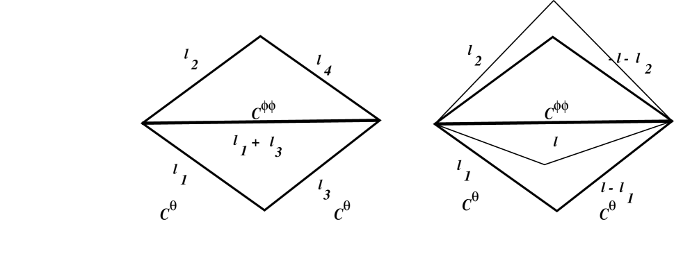
FIG. 1.: Left: The lensing trispectrum configuration, following equation (37), where the diagonal of the configuration contains information related to lensing while the sides of the quadrilateral contain information related to primary anisotropy power spectra at the last scattering surface. Right: This lensing information can be extracted by a statistic that effectively probes the diagonal, such as the power spectrum of squared temperatures discussed here. This statistic sums over all quadrilateral configurations, as indicated by thin lines, for a given length of the diagonal. As we find later, the lensing information associated with the other — vertical in this diagram — diagonal, proportional to $C_{|{\bf l}_{1}+{\bf l}_{2}|}^{\phi\phi}$, acts as a source of non-Gaussian noise in this extraction. The other contribution to the non-Gaussian noise, through a term proportional to $C_{|{\bf l}-{\bf l}_{1}+{\bf l}_{2}|}$, comes from interchanging ${\bf l}_{1}$ with ${\bf l}-{\bf l}_{1}$, which alters the vertical diagonal while keeping the horizontal diagonal fixed.

IV Power spectrum of squared temperatures

As written in equation (37), the trispectrum formed by lensing alone depends on the power spectrum of deflection angle. Thus, with the right configuration for the CMB trispectrum, one can hope to extract some information related to lensing, mainly $C_{l}^{\phi\phi}$, given some knowledge on CMB anisotropies, such as $C_{l}^{\Theta}$. Note that a contribution to the CMB trispectrum due to lensing comes from $C_{l}^{\phi\phi}$ when $l=|{\bf l}_{i}+{\bf l}_{j}|$ when ${\bf l}_{i}$ and ${\bf l}_{j}$ are the two sides of the quadrilateral that form the trispectrum. As illustrated in figure (1), this is equivalent to the diagonal of the quadrilateral and can be probed easily with a statistic that averages over the configurations for a given length of the diagonal. For this purpose, an useful option is to consider the configurations of the trispectrum that contribute to the power spectrum of squared temperatures. To see why such a statistic probe the diagonal of the trispectrum, consider the definition of this squared power spectrum

$$\langle\tilde{\Theta}^{2}({\bf l})\tilde{\Theta}^{2}({\bf l}^{\prime})\rangle=(2\pi)^{2}\delta_{D}({\bf l}+{\bf l}^{\prime})C_{l}^{2}\,,$$ (45)

where the Fourier transform of the squared temperature can be written as a convolution of the temperature transforms

$$\tilde{\Theta}^{2}({\bf l})=\int\frac{d^{2}{\bf l}_{1}}{(2\pi)^{2}}\tilde{\Theta}({\bf l}_{1})\tilde{\Theta}({\bf l}-{\bf l}_{1})\,.$$ (46)

Here, it should be understood that $\tilde{\Theta}^{2}({\bf l})$ refers to the Fourier transform of the square of the temperature rather than square of the Fourier transform of temperature, $[\tilde{\Theta}({\bf l})]^{2}$. Note that the Fourier transform of the temperature fluctuation, in the flat sky, is

$$\tilde{\Theta}({\bf l})=\int d^{2}\theta e^{-i{\bf l}\cdot\theta}\tilde{T}(\theta)\,.$$ (47)

To compute the squared power spectrum of CMB temperature, we take

$$\langle\tilde{\Theta}^{2}({\bf l})\tilde{\Theta}^{2}({\bf l}^{\prime})\rangle = (2\pi)^{2}\delta_{D}({\bf l}+{\bf l}^{\prime})C_{l}^{2}\,$$ (48)

$$= \int\frac{d^{2}{\bf l}_{1}}{(2\pi)^{2}}\int\frac{d^{2}{\bf l}_{2}}{(2\pi)^{2}}\langle\tilde{\Theta}({\bf l}_{1})\tilde{\Theta}({\bf l}-{\bf l}_{1})\tilde{\Theta}({\bf l}_{2})\tilde{\Theta}({\bf l}^{\prime}-{\bf l}_{2})\rangle\,.$$ (49)

Since the lensing power spectrum contributes to the above squared power spectrum via the diagonals of the quadrilateral, the power spectrum of squared temperatures contain terms which are simply proportional to $C_{l}^{\phi\phi}$ where $l$ is the multipole at which the squared power spectrum is measured. As discussed in [8], this then allows an extraction of the angular power spectrum of lensing deflections.

There is also a dominant noise contribution to the squared power spectrum. This noise contribution comes from the lowest order correlations and is present even in the presence of Gaussian temperature fluctuations; thus, we denote it as the Gaussian noise contribution. In the presence of the non-Gaussian contribution resulting from the lensing effect, we write these two contributions as

$$C_{l}^{2}=C_{l}^{\rm G}+C_{l}^{\rm NG}\,,$$ (51)

with

$$C_{l}^{2\rm G}=\int\frac{d^{2}{\bf l}_{1}}{(2\pi)^{2}}2C_{l_{1}}^{\rm t}C_{|{\bf l}-{\bf l}_{1}|}^{\rm t}\,,$$ (52)

and the non-Gaussianity captured by the four-point correlator as

$$C_{l}^{2\rm NG}=\int\frac{d^{2}{\bf l}_{1}}{(2\pi)^{2}}\int\frac{d^{2}{\bf l}_{2}}{(2\pi)^{2}}\tilde{T}({\bf l}_{1},{\bf l}-{\bf l}_{1},{\bf l}_{2},-{\bf l}-{\bf l}_{2})\,.$$ (53)

.

Following our previous discussion on the lensing trispectrum, we can now write the full four-point contribution to the squared power spectrum — by replacing ${\bf l}_{1},{\bf l}_{2},{\bf l}_{3}$ and ${\bf l}_{4}$ in equation (37) with the required configuration from above — such that

$$C_{l}^{2\rm NG}=C_{l}^{\phi\phi}\left[\int{d^{2}{\bf l}_{1}\over(2\pi)^{2}}{\bf l}\cdot{\bf l}_{1}C^{\Theta}_{l_{1}}+{\bf l}\cdot({\bf l}-{\bf l}_{1})C^{\Theta}_{|{\bf l}-{\bf l}_{1}|}\right]^{2}$$ (54)

$$+ \int{d^{2}{\bf l}_{1}\over(2\pi)^{2}}\int{d^{2}{\bf l}_{2}\over(2\pi)^{2}}\Big{\{}C_{|{\bf l}_{1}+{\bf l}_{2}|}^{\phi\phi}[{\bf l}_{1}\cdot({\bf l}_{1}+{\bf l}_{2})C^{\Theta}_{l_{1}}+{\bf l}_{2}\cdot({\bf l}_{1}+{\bf l}_{2})C^{\Theta}_{l_{2}}][({\bf l}+{\bf l}_{2})\cdot({\bf l}_{1}+{\bf l}_{2})C^{\Theta}_{|{\bf l}+{\bf l}_{2}|}-({\bf l}_{1}+{\bf l}_{2})\cdot({\bf l}-{\bf l}_{1})C^{\Theta}_{|{\bf l}-{\bf l}_{1}|}]$$ (55)

$$+ C_{|{\bf l}-{\bf l}_{1}+{\bf l}_{2}|}^{\phi\phi}[({\bf l}-{\bf l}_{1}+{\bf l}_{2})\cdot{\bf l}_{2}C^{\Theta}_{l_{2}}+({\bf l}-{\bf l}_{1}+{\bf l}_{2})\cdot({\bf l}-{\bf l}_{1})C^{\Theta}_{|{\bf l}-{\bf l}_{1}|}][-({\bf l}-{\bf l}_{1}+{\bf l}_{2})\cdot{\bf l}_{1}C^{\Theta}_{l_{1}}+({\bf l}-{\bf l}_{1}+{\bf l}_{2})\cdot({\bf l}+{\bf l}_{2})C^{\Theta}_{|{\bf l}+{\bf l}_{2}|}]\Big{\}}\,.$$ (56)

FIG. 2.: Optimal filter function $W({\bf l}_{1}+{\bf l}_{2},{\bf l}_{1})$ for the extraction of $C_{l}^{\phi\phi}$ from the CMB²-CMB² power spectrum as a function of $l_{1}$ and $l_{2}$. The angle between ${\bf l}_{1}$ and ${\bf l}_{2}$ is constrained by the fixed value of $l=|{\bf l}_{1}+{\bf l}_{2}|$ in each plot. The left plot $(l=100)$ and right plot $(l=2000)$ correspond to large and small angular scales respectively. The optimal filter removes excess noise at multipoles less than $\sim$ 1500 and is weighted to exploit the sensitivity to lensing of the damping tail.

As written, and discussed above, one of the terms in the non-Gaussian contribution to the squared power spectrum is directly proportional to $C_{l}^{\phi\phi}$. To extract this angular power spectrum of lensing deflections, consider the approach suggested by [8] involving the quadratic statistics formed by the divergence of the temperature-weighted gradients. To understand the mechanism involved, consider a filtered version of the squared power spectrum such that

$$\hat{\Theta}^{2}({\bf l})=\int\frac{d^{2}{\bf l}_{1}}{(2\pi)^{2}}W({\bf l},{\bf l}_{1})\tilde{\Theta}({\bf l}_{1})\tilde{\Theta}({\bf l}-{\bf l}_{1})\,,$$ (58)

where $W$ is a filter that acts on the CMB temperature. This filtering can be either in real space or Fourier, or multipolar, space. For simplicity, we have introduced filters that are applicable in Fourier space. To extract the optimal filter in the presence of the Gaussian noise alone, we ignore the additional noise contribution from the second and third terms of the trispectrum involving integrals over $C_{|{\bf l}_{1}+{\bf l}_{2}|}^{\phi\phi}$ and $C_{|{\bf l}-{\bf l}_{1}+{\bf l}_{2}|}^{\phi\phi}$.

We can, thus, write the filtered version of the squared power spectrum as

$$\hat{C}_{l}^{2} = \int\frac{d^{2}{\bf l}_{1}}{(2\pi)^{2}}C_{l_{1}}^{\rm t}C_{|{\bf l}-{\bf l}_{1}|}^{\rm t}W({\bf l},{\bf l}_{1})\left[W(-{\bf l},-{\bf l}_{1})+W(-{\bf l},{\bf l}_{1}-{\bf l})\right]$$ (59)

$$+ C_{l}^{\phi\phi}\left[\int\frac{d^{2}{\bf l}_{1}}{(2\pi)^{2}}W({\bf l},{\bf l}_{1})[{\bf l}\cdot{\bf l}_{1}C^{\Theta}_{l_{1}}+{\bf l}\cdot({\bf l}-{\bf l}_{1})C^{\Theta}_{|{\bf l}-{\bf l}_{1}|}]\right]\left[\int\frac{d^{2}{\bf l}_{1}}{(2\pi)^{2}}W(-{\bf l},-{\bf l}_{1})[{\bf l}\cdot{\bf l}_{1}C^{\Theta}_{l_{1}}+{\bf l}\cdot({\bf l}-{\bf l}_{1})C^{\Theta}_{|{\bf l}-{\bf l}_{1}|}]\right].$$ (60)

We assume that our filter has the symmetry property $W({\bf l},{\bf l}_{1})=W(-{\bf l},-{\bf l}_{1})=W(-{\bf l},{\bf l}_{1}-{\bf l})$ and then check to see if this assumption is justified. To be consistent with prior results, we also make one more assumption here. We take the Gaussian noise to be the dominant noise contribution and ignore the noise from the two extra terms in the non-Gaussian trispectrum that involves integrals over $C^{\phi\phi}_{|{\bf l}_{1}+{\bf l}_{2}|}$ and $C^{\phi\phi}_{|{\bf l}-{\bf l}_{1}+{\bf l}_{2}|}$. Thus, the filter we will derive here is only optimal in the presence of the dominant Gaussian noise and is sub-optimal when all noise terms are considered. We will later add in these two terms as an extra source of noise, with the filter derived by ignoring them applied appropriately.

With these assumptions, we can write the signal-to-noise ratio for the detection of the $\phi$ power spectrum per each multipole moment as,

$$\left(\frac{{\rm S}}{{\rm N}}\right)^{2}=\frac{(2l+1)}{2}\left(\frac{C_{l}^{\phi\phi}\left[\int\frac{d^{2}{\bf l}_{1}}{(2\pi)^{2}}W({\bf l},{\bf l}_{1})[{\bf l}\cdot{\bf l}_{1}C^{\Theta}_{l_{1}}+{\bf l}\cdot({\bf l}-{\bf l}_{1})C^{\Theta}_{|{\bf l}-{\bf l}_{1}|}]\right]^{2}}{C_{l}^{\phi\phi}\left[\int\frac{d^{2}{\bf l}_{1}}{(2\pi)^{2}}W({\bf l},{\bf l}_{1})[{\bf l}\cdot{\bf l}_{1}C^{\Theta}_{l_{1}}+{\bf l}\cdot({\bf l}-{\bf l}_{1})C^{\Theta}_{|{\bf l}-{\bf l}_{1}|}]\right]^{2}+\int\frac{d^{2}{\bf l}_{1}}{(2\pi)^{2}}W({\bf l},{\bf l}_{1})^{2}2C_{l_{1}}^{\rm t}C_{|{\bf l}-{\bf l}_{1}|}^{\rm t}}\right)^{2}\,.$$ (62)

The optimal filter in the presence of Gaussian noise is the one that will maximize this ratio.

FIG. 3.: The extraction of the lensing power spectrum from temperature data alone. We show the dominant Gaussian noise (top lines) and the noise associated with the extra terms in the trispectrum due to lensing alone (bottom lines). The curves are for three values of the resolution in the CMB temperature map with an effective sensitivity of 1 $\mu$K $\sqrt{\rm sec}$.

To extract the required filter, we take derivatives with respect to $W$ and find that the maximum is satisfied when

$$W({\bf l},{\bf l}_{1})=\frac{[{\bf l}\cdot{\bf l}_{1}C_{l_{1}}^{\Theta}+{\bf l}\cdot({\bf l}-{\bf l}_{1})C_{|{\bf l}-{\bf l}_{1}|}^{\Theta}]}{2C_{l_{1}}^{\rm t}C_{|{\bf l}-{\bf l}_{1}|}^{\rm t}}\,.$$ (63)

Performing the explicit substitutions ${\bf l}\to-{\bf l},{\bf l}_{1}\to-{\bf l}_{1}$ and ${\bf l}\to-{\bf l},{\bf l}_{1}\to{\bf l}_{1}-{\bf l}$, we see that our optimal filter does possess the desired symmetry. We introduced this filter in Ref. [33] when discussing the CMB²-SZ power spectrum as a way to extract the lensing-SZ correlation directly using the power spectrum of squared temperature and temperature. It is not a surprise that the same filter appears now when extracting the lensing-lensing correlations using the power spectrum of squared temperature and squared temperature. A physical mechanism to achieve this filter in real space is presented in Ref. [20] by taking the gradient of the temperature, weighting it by a noise filtered CMB map, then taking the divergence of this product.

With the filter applied, we get a direct estimator of $C_{l}^{\phi\phi}$. Introducing,

$$N_{l}^{-1}\equiv\int\frac{d^{2}{\bf l}_{1}}{(2\pi)^{2}}\frac{[{\bf l}\cdot{\bf l}_{1}C^{\Theta}_{l_{1}}+{\bf l}\cdot({\bf l}-{\bf l}_{1})C^{\Theta}_{|{\bf l}-{\bf l}_{1}|}]^{2}}{2C_{l_{1}}^{\rm t}C_{|{\bf l}-{\bf l}_{1}|}^{\rm t}}$$ (64)

(65)

The filtered squared power spectrum is such that

$$N_{l}^{2}\hat{C}_{l}^{2}=N_{l}+C_{l}^{\phi\phi}\,,$$ (66)

where the Gaussian noise associated with the extracted $C_{l}^{\phi\phi}$ is $N_{l}$.

We can now add in the noise contribution arising from the two extra terms in the non-Gaussian trispectrum which we dropped when deriving the optimal filter in the presence of the Gaussian noise only. This extra noise contribution, neglected in prior studies, is

$$N_{l}^{\rm NG}=N_{l}^{2}\int\frac{d^{2}{\bf l}_{1}}{(2\pi)^{2}}\int\frac{d^{2}{\bf l}_{2}}{(2\pi)^{2}}W({\bf l},{\bf l}_{1})W(-{\bf l},{\bf l}_{2})$$ (68)

$$\Big{\{}C_{|{\bf l}_{1}+{\bf l}_{2}|}^{\phi\phi}[{\bf l}_{1}\cdot({\bf l}_{1}+{\bf l}_{2})C^{\Theta}_{l_{1}}+{\bf l}_{2}\cdot({\bf l}_{1}+{\bf l}_{2})C^{\Theta}_{l_{2}}][({\bf l}+{\bf l}_{2})\cdot({\bf l}_{1}+{\bf l}_{2})C^{\Theta}_{|{\bf l}+{\bf l}_{2}|}-({\bf l}_{1}+{\bf l}_{2})\cdot({\bf l}-{\bf l}_{1})C^{\Theta}_{|{\bf l}-{\bf l}_{1}|}]$$

$$+ C_{|{\bf l}-{\bf l}_{1}+{\bf l}_{2}|}^{\phi\phi}[({\bf l}-{\bf l}_{1}+{\bf l}_{2})\cdot{\bf l}_{2}C^{\Theta}_{l_{2}}+({\bf l}-{\bf l}_{1}+{\bf l}_{2})\cdot({\bf l}-{\bf l}_{1})C^{\Theta}_{|{\bf l}-{\bf l}_{1}|}][-({\bf l}-{\bf l}_{1}+{\bf l}_{2})\cdot{\bf l}_{1}C^{\Theta}_{l_{1}}+({\bf l}-{\bf l}_{1}+{\bf l}_{2})\cdot({\bf l}+{\bf l}_{2})C^{\Theta}_{|{\bf l}+{\bf l}_{2}|}]\Big{\}}\,.$$ (69)

With the non-Gaussian noise, we can write

$$N_{l}^{2}\hat{C}_{l}^{2}=N_{l}+N_{l}^{\rm NG}+C_{l}^{\phi\phi}\,.$$ (71)

There is a strong possibility that the noise-bias $N_{l}$ associated with the Gaussian contribution to the squared power spectrum can be removed during the lensing reconstruction. This would involve the construction of a new estimator of lensing, or filtering scheme, that removes $N_{l}$ and leaves $N_{l}^{\rm NG}$ as the final noise contribution associated with the reconstructed $C_{l}^{\phi\phi}$. The removal of the dominant Gaussian noise bias is extremely useful since this allows one to lower the noise contribution associated with $C_{l}^{\phi\phi}$ by at least an order of magnitude. We will return later to the impact of such a noise-bias removal on the identification of an inflationary gravitational wave signature in the CMB in the form of a curl (or B-mode) contribution to the polarization.

In addition to the additional non-Gaussian noise contribution from the lensing trispectrum itself, there is an additional noise contribution resulting from the relevant configuration of the trispectrum due to lensing-secondary correlations. We do not reproduce this contribution here, but it can be easily calculated by replacing $({\bf l}_{1},{\bf l}_{2},{\bf l}_{3},{\bf l}_{4})$ in equation (44), with $({\bf l}_{1},{\bf l}-{\bf l}_{1},{\bf l}_{2},-{\bf l}-{\bf l}_{2})$. Note that this additional noise results from the correlation between potentials that deflect CMB photons and the secondary contributions associated with the ISW and SZ thermal effects. In the presence of such contributions, we also note that $C_{l}^{\rm t}$ in equation (65), contains all contributions to noise, including the secondary contribution. It is well known that certain secondary contributions can be removed based on distinct signatures, such as the spectral dependence of the SZ effect [15]. In such cases, we expect only the lensing-ISW correlation to produce a noise contribution. This effect is small and can be easily ignored. In the presence of the SZ contribution, however, there is a significant noise contribution that can potentially limit the extraction of the lensing power spectrum.

Note that the filter is symmetric in ${\bf l}_{1}$ and ${\bf l}-{\bf l}_{1}$. We show surfaces of this filter in figure (2) as a function of $l_{1}$ and $l_{2}=|{\bf l}-{\bf l}_{1}|$ for two values of $l$ corresponding to large and small angular scales respectively. As shown, the filter behaves such that information related to lensing is extracted at arcminute scales via the damping tail of the CMB anisotropies. Additionally, since lensing smooths the acoustic peak structure, further information is also extracted in a subtle way from fluctuations associated with large angular scales. Thus, a simple filter which effectively cuts off the acoustic peak structure but extracts information from small angular scales, such a a step function in multipolar space, does poorly when compared to the filtering scheme proposed above [33]. As mentioned before deriving the filter, it should be noted that the proposed filter is only optimal to the extent that Gaussian noise contribution is dominant. In the presence of noise contributions from additional four-point correlations or, more importantly, additional terms in the lensing trispectrum itself, the filter is sub-optimal. We failed to find a simple analytical description for an optimal filter that also suppresses the non-Gaussian noise contribution from the additional terms in the lensing trispectrum. As we find later, since these terms only contribute at an order of magnitude below the dominant Gaussian noise, we do not expect this to be a significant problem in the extraction of the lensing information.

V The EB Trispectrum

In addition to temperature, lensing also affects the CMB polarization. We discuss here the best estimator from polarization observables for extracting the lensing contribution following the discussion in Ref. [21] and provide relevant equations for other estimators in the Appendix. The statistic considered in this section involves the squared map constructed by convolving, in Fourier space, the E- and B-mode maps of the polarization. We denote this by $(EB)({\bf l})$. To understand this combination, we consider the Fourier space analogue and, as before, write,

$$EB({\bf l})=\frac{1}{2}\int\frac{d^{2}{\bf l}_{1}}{(2\pi)^{2}}\left[E({\bf l}_{1})B({\bf l}-{\bf l}_{1})+B({\bf l}_{1})E({\bf l}-{\bf l}_{1})\right]\,.$$ (72)

Now considering the power spectrum formed by $\langle EB({\bf l})EB({\bf l}^{\prime})\rangle=(2\pi)^{2}\delta({\bf l}+{\bf l}^{\prime})C_{l}^{(EB)^{2}}$, we write

$$\langle EB({\bf l})EB({\bf l}^{\prime})\rangle=\frac{1}{4}\int\frac{d^{2}{\bf l}_{1}}{(2\pi)^{2}}\int\frac{d^{2}{\bf l}_{2}}{(2\pi)^{2}}\langle\left[E({\bf l}_{1})B({\bf l}-{\bf l}_{1})+B({\bf l}_{1})E({\bf l}-{\bf l}_{1})\right]\left[E({\bf l}_{2})B({\bf l}^{\prime}-{\bf l}_{2})+B({\bf l}_{2})E({\bf l}^{\prime}-{\bf l}_{2})\right]\rangle\,.$$ (73)

Here, again, we find two sources of contributions, involving a noise contribution due to Gaussian fluctuations in the E- and B-maps,

$$C_{l}^{(EB)^{2}\rm G}=\frac{1}{4}\int\frac{d^{2}{\bf l}_{1}}{(2\pi)^{2}}\left[2C_{l_{1}}^{EE{\rm t}}C_{|{\bf l}-{\bf l}_{1}|}^{BB{\rm t}}+2C_{l_{1}}^{BB{\rm t}}C_{|{\bf l}-{\bf l}_{1}|}^{EE{\rm t}}\right]\,,$$ (74)

and a non-Gaussian contribution due to the lensing effect on polarization.

FIG. 4.: The extraction of lensing power spectrum from temperature data in the presence of foregrounds (mainly the thermal SZ effect). The increase in dominant Gaussian noise (top lines) is due to the extra SZ power spectrum, which peaks at small angular scales. The dot-dashed line is the resulting non-Gaussian noise contribution due to the trispectrum formed by the SZ-lensing cross-correlation.

FIG. 5.: The extraction of lensing power spectrum from polarization data. We show the associated noise due to the dominant Gaussian noise (top lines) and noise due to extra terms in the trispectrum (bottom lines). The curves are for a resolution of 5 arcmin in the CMB temperature map with an effective sensitivity of 1 $\mu$K $\sqrt{\rm sec}$. As shown, the EB estimator probes the lensing potential power spectrum to smaller angular scales than the quadratic estimator on temperature data alone or estimators based on other combinations of polarization and the temperature.

To calculate the lensing contribution to the polarization, we follow the notation in Ref. [12]. Introducing,

$${}_{\pm}\tilde{X}(\hat{\bf n}) = {}_{\pm}X(\hat{\bf n}+\nabla\phi)$$ (75)

$$\approx {}_{\pm}X(\hat{\bf n})+\nabla_{i}\phi(\hat{\bf n})\nabla^{i}{}_{\pm}X(\hat{\bf n})+{1\over 2}\nabla_{i}\phi(\hat{\bf n})\nabla_{j}\phi(\hat{\bf n})\nabla^{i}\nabla^{j}{}_{\pm}X(\hat{\bf n})\,,$$ (76)

where $\,{}_{\pm}^{\vphantom{m}}X=Q\pm iU$ represent combinations of the Stokes parameters. The lensing effect is again to move the photon propagation directions on the sky. In Fourier space, we can consider the E- and B-mode decomposition introduced in Ref. [17] such that ${}_{\pm}X({\bf l})=E({\bf l})\pm iB({\bf l})$ and

$${}_{\pm}\tilde{X}({\bf l}) = {}_{\pm}X({\bf l})-\int{d^{2}{\bf l}_{1}\over(2\pi)^{2}}{}_{\pm}X({{\bf l}_{1}})e^{\pm 2i(\varphi_{{\bf l}_{1}}-\varphi_{{\bf l}})}L({\bf l},{\bf l}_{1})\,.$$ (77)

With this, we can write

$$\tilde{E}({\bf l}) = E({\bf l})-\int{d^{2}{\bf l}_{1}\over(2\pi)^{2}}\left[E({\bf l}_{1})\cos 2(\varphi_{{\bf l}_{1}}-\varphi_{\bf l})-B({\bf l}_{1})\sin 2(\varphi_{{\bf l}_{1}}-\varphi_{\bf l})\right]\phi({\bf l}-{\bf l}_{1})({\bf l}-{\bf l}_{1})\cdot{\bf l}_{1}$$ (78)

$$\tilde{B}({\bf l}) = B({\bf l})-\int{d^{2}{\bf l}_{1}\over(2\pi)^{2}}\left[E({\bf l}_{1})\sin 2(\varphi_{{\bf l}_{1}}-\varphi_{\bf l})+B({\bf l}_{1})\cos 2(\varphi_{{\bf l}_{1}}-\varphi_{\bf l})\right]\phi({\bf l}-{\bf l}_{1})({\bf l}-{\bf l}_{1})\cdot{\bf l}_{1}\,,$$ (79)

Since primordial $B({\bf l})$, due to the gravitational wave contribution, is small, we can make the useful approximation that

$$\tilde{E}({\bf l}) = E({\bf l})-\int{d^{2}{\bf l}_{1}\over(2\pi)^{2}}\left[E({\bf l}_{1})\cos 2(\varphi_{{\bf l}_{1}}-\varphi_{\bf l})\right]\phi({\bf l}-{\bf l}_{1})({\bf l}-{\bf l}_{1})\cdot{\bf l}_{1}$$ (80)

$$\tilde{B}({\bf l}) = -\int{d^{2}{\bf l}_{1}\over(2\pi)^{2}}\left[E({\bf l}_{1})\sin 2(\varphi_{{\bf l}_{1}}-\varphi_{\bf l})\right]\phi({\bf l}-{\bf l}_{1})({\bf l}-{\bf l}_{1})\cdot{\bf l}_{1}\,,$$ (81)

Under this approximation, the lensed polarization power spectra can be expressed in terms of $C_{l}^{\phi\phi}$ and the unlensed quantities following Ref. [12]:

$$\tilde{C}_{l}^{EE} = \left[1-\int{d^{2}{\bf l}_{1}\over(2\pi)^{2}}C^{\phi\phi}_{l_{1}}\left({\bf l}_{1}\cdot{\bf l}\right)^{2}\right]\,C_{l}^{EE}+\frac{1}{2}\int{d^{2}{\bf l}_{1}\over(2\pi)^{2}}C_{|{\bf l}-{\bf l}_{1}|}^{\phi\phi}[({\bf l}-{\bf l}_{1})\cdot{\bf l}_{1}]^{2}C^{EE}_{l_{1}}[1+\cos(4\varphi_{{\bf l}_{1}})]\,,$$ (82)

$$\tilde{C}_{l}^{BB} = \frac{1}{2}\int{d^{2}{\bf l}_{1}\over(2\pi)^{2}}C_{|{\bf l}-{\bf l}_{1}|}^{\phi\phi}[({\bf l}-{\bf l}_{1})\cdot{\bf l}_{1}]^{2}C^{EE}_{l_{1}}[1-\cos(4\varphi_{{\bf l}_{1}})]\,.$$ (83)

The total polarization power spectra is the sum of these lensed spectra and a noise contribution

$$C_{l}^{EE{\rm t}}=\tilde{C}_{l}^{EE}+C_{l}^{\rm n}\,\quad\quad C_{l}^{BB{\rm t}}=\tilde{C}_{l}^{BB}+C_{l}^{\rm n},$$ (85)

where the noise component is given by equation (31) with a possibly different NET $s$ for polarization.

With the lensing effect on $B({\bf l})$, we can now calculate the trispectrum contribution to the squared power spectrum as

$$C_{l}^{(EB)^{2}\rm NG}=-\frac{1}{4}C_{l}^{\phi\phi}\left[\int{d^{2}{\bf l}_{1}\over(2\pi)^{2}}\Big{\{}C_{l_{1}}^{EE}{\bf l}\cdot{\bf l}_{1}+C_{|{\bf l}-{\bf l}_{1}|}^{EE}{\bf l}\cdot({\bf l}-{\bf l}_{1})\Big{\}}\sin 2(\varphi_{{\bf l}_{1}}+\varphi_{{\bf l}-{\bf l}_{1}})\right]^{2}$$ (86)

$$+ \int{d^{2}{\bf l}_{1}\over(2\pi)^{2}}\int{d^{2}{\bf l}_{2}\over(2\pi)^{2}}\Big{\{}\frac{1}{4}C_{|{\bf l}_{1}+{\bf l}_{2}|}^{\phi\phi}\left[C_{l_{1}}^{EE}C_{|{\bf l}+{\bf l}_{2}|}^{EE}({\bf l}_{1}+{\bf l}_{2})\cdot({\bf l}+{\bf l}_{2})({\bf l}_{1}+{\bf l}_{2})\cdot{\bf l}_{1}-C_{l_{2}}^{EE}C_{|{\bf l}-{\bf l}_{1}|}^{EE}({\bf l}_{1}+{\bf l}_{2})\cdot{\bf l}_{2}({\bf l}_{1}+{\bf l}_{2})\cdot({\bf l}-{\bf l}_{1})\right]$$ (88)

$$\quad\quad\times\sin 2(\varphi_{{\bf l}-{\bf l}_{1}}-\varphi_{{\bf l}+{\bf l}_{2}})\sin 2(\varphi_{{\bf l}_{1}}+\varphi_{{\bf l}_{2}})$$

$$+ \frac{1}{4}C_{|{\bf l}-{\bf l}_{1}+{\bf l}_{2}|}^{\phi\phi}\left[C_{|{\bf l}-{\bf l}_{1}|}^{EE}C_{|{\bf l}+{\bf l}_{2}|}^{EE}({\bf l}-{\bf l}_{1}+{\bf l}_{2})\cdot({\bf l}+{\bf l}_{2})({\bf l}-{\bf l}_{1}+{\bf l}_{2})\cdot({\bf l}-{\bf l}_{1})-C_{l_{1}}^{EE}C_{l_{2}}^{EE}({\bf l}-{\bf l}_{1}+{\bf l}_{2})\cdot{\bf l}_{1}({\bf l}-{\bf l}_{1}+{\bf l}_{2})\cdot{\bf l}_{2}\right]$$ (90)

$$\quad\quad\times\sin 2(\varphi_{{\bf l}_{1}}-\varphi_{{\bf l}+{\bf l}_{2}})\sin 2(\varphi_{{\bf l}-{\bf l}_{1}}+\varphi_{{\bf l}_{2}})\Big{\}}\,,$$

To extract the lensing contribution, one can again consider a filtering scheme, and following arguments similar to the case with temperature, the derived filter that maximizes the signal-to-noise in the presence of Gaussian noise is

$$W({\bf l},{\bf l}_{1})=\frac{\left[C_{l_{1}}^{EE}{\bf l}\cdot{\bf l}_{1}+C_{|{\bf l}-{\bf l}_{1}|}^{EE}{\bf l}\cdot({\bf l}-{\bf l}_{1})\right]\sin 2(\varphi_{{\bf l}_{1}}+\varphi_{{\bf l}-{\bf l}_{1}})}{C_{l_{1}}^{EE{\rm t}}C_{|{\bf l}-{\bf l}_{1}|}^{BB{\rm t}}+C_{l_{1}}^{BB{\rm t}}C_{|{\bf l}-{\bf l}_{1}|}^{EE{\rm t}}}\,.$$ (91)

With this filter applied, the associated noise due to the dominant Gaussian part is $N_{l}$, where,

$$N_{l}^{-1}=\int{d^{2}{\bf l}_{1}\over(2\pi)^{2}}\frac{\left[C_{l_{1}}^{EE}{\bf l}\cdot{\bf l}_{1}+C_{|{\bf l}-{\bf l}_{1}|}^{EE}{\bf l}\cdot({\bf l}-{\bf l}_{1})\right]^{2}\sin^{2}2(\varphi_{{\bf l}_{1}}+\varphi_{{\bf l}-{\bf l}_{1}})}{2C_{l_{1}}^{EE{\rm t}}C_{|{\bf l}-{\bf l}_{1}|}^{BB{\rm t}}+2C_{l_{1}}^{BB{\rm t}}C_{|{\bf l}-{\bf l}_{1}|}^{EE{\rm t}}}\,.$$ (92)

The extra noise due to the additional terms in the trispectrum is

$$N_{l}^{\rm NG} = N_{l}^{2}\int{d^{2}{\bf l}_{1}\over(2\pi)^{2}}\int{d^{2}{\bf l}_{2}\over(2\pi)^{2}}W({\bf l},{\bf l}_{1})W(-{\bf l},{\bf l}_{2})\Big{\{}$$ (93)

$$\times \frac{1}{4}C_{|{\bf l}_{1}+{\bf l}_{2}|}^{\phi\phi}\left[C_{l_{1}}^{EE}C_{|{\bf l}+{\bf l}_{2}|}^{EE}({\bf l}_{1}+{\bf l}_{2})\cdot({\bf l}+{\bf l}_{2})({\bf l}_{1}+{\bf l}_{2})\cdot{\bf l}_{1}-C_{l_{2}}^{EE}C_{|{\bf l}-{\bf l}_{1}|}^{EE}({\bf l}_{1}+{\bf l}_{2})\cdot{\bf l}_{2}({\bf l}_{1}+{\bf l}_{2})\cdot({\bf l}-{\bf l}_{1})\right]$$ (95)

$$\quad\quad\times\sin 2(\varphi_{{\bf l}-{\bf l}_{1}}-\varphi_{{\bf l}+{\bf l}_{2}})\sin 2(\varphi_{{\bf l}_{1}}+\varphi_{{\bf l}_{2}})$$

$$+ \frac{1}{4}C_{|{\bf l}-{\bf l}_{1}+{\bf l}_{2}|}^{\phi\phi}\left[C_{|{\bf l}-{\bf l}_{1}|}^{EE}C_{|{\bf l}+{\bf l}_{2}|}^{EE}({\bf l}-{\bf l}_{1}+{\bf l}_{2})\cdot({\bf l}+{\bf l}_{2})({\bf l}-{\bf l}_{1}+{\bf l}_{2})\cdot({\bf l}-{\bf l}_{1})-C_{l_{1}}^{EE}C_{l_{2}}^{EE}({\bf l}-{\bf l}_{1}+{\bf l}_{2})\cdot{\bf l}_{1}({\bf l}-{\bf l}_{1}+{\bf l}_{2})\cdot{\bf l}_{2}\right]$$ (97)

$$\quad\quad\times\sin 2(\varphi_{{\bf l}_{1}}-\varphi_{{\bf l}+{\bf l}_{2}})\sin 2(\varphi_{{\bf l}-{\bf l}_{1}}+\varphi_{{\bf l}_{2}})\Big{\}}\,.$$

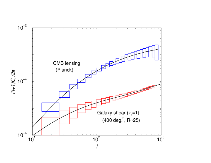
FIG. 6.: Left: Weak lensing as a CMB experiment. We show errors for the reconstruction of convergence, or projected mass density, to the last scattering surface with Planck temperature data. This is compared to the convergence measurements expected from observations of galaxy ellipticities which probe to redshifts of $\sim$ 1 to 2. Right: The cumulative signal-to-noise ratio for the detection of the lensing effect in Planck data, using the filtered squared temperature statistic discussed here (solid line) and the gradient statistic (dotted line) described in Ref. [14] . The dot-dashed line is the cumulative signal-to-noise ratio when the dominant Gaussian noise is removed as part of the lensing reconstruction. With such a removal, the noise in the lensing reconstruction is determined by the non-Gaussian contributions which are roughly an order of magnitude below the Gaussian noise level.

VI Discussion

We have introduced the trispectrum, or four-point correlation function, of CMB anisotropies as a probe of the large scale structure weak lensing effect. The trispectrum in CMB anisotropies is generated by the non-linear mode coupling behavior of the weak lensing effect on the CMB. As written in equation (37), the trispectrum formed by lensing contains a significant contribution from $C_{l}^{\phi\phi}$ when $l=|{\bf l}_{1}+{\bf l}_{3}|$. ${\bf l}_{1}$ and ${\bf l}_{3}$ are the two sides of the quadrilateral that formed the trispectrum in the Fourier space as illustrated in figure 1. Contributions thus probe the lensing effect via the diagonal of the trispectrum configuration, and statistics sensitive to the diagonal will provide a practical approach for extracting the lensing angular power spectrum.

A useful statistic for this purpose is the power spectrum formed by squared temperatures introduced earlier. This approach expands the suggestion in Ref. [33] to use the squared temperature-temperature power spectrum to study the CMB bispectrum and a filtered version to extract the power spectrum associated with lensing-SZ correlation. The power spectrum formed by squared temperatures probes the trispectrum. This power spectrum, however, contains a dominant contribution due to the Gaussian fluctuations associated with temperature which potentially dominates the contribution arising from the non-Gaussian weak lensing effect. To optimally extract the lensing contribution in the presence of this dominant Gaussian noise, we have introduced a filter in Fourier space. This filter requires knowledge of the noise contributions to the map as well as the power spectra of prelensed primary anisotropies at the last scattering surface. Though the filter can be easily applied to the Fourier transform of the squared temperature map in the Fourier space, a useful direct approach is presented in Ref. [20]. This real space construction involves the divergence of the temperature-weighted temperature gradients, with each of these temperature estimators first filtered for the excess noise.

We have extended the previous discussions of the extraction of lensing signal to include a discussion of the full trispectrum. The full trispectrum contains terms which were previously ignored and these terms contribute as additional sources of noise in the lensing reconstruction and can potentially interfere with the extraction of the lensing signal from CMB data. These additional non-Gaussian noise terms correspond to the lensing contribution associated with the second diagonal of the trispectrum configuration shown in figure (1) and the same diagonal under a permutation, while keeping the same vector ${\bf l}$ for the diagonal from which lensing information is extracted. In figure (3), we summarize our results related to the lensing extraction using temperature data alone. We show the dominant Gaussian noise contribution and the associated non-Gaussian noise contribution, due to the two additional terms in the trispectrum which involve integrals over $C^{\phi\phi}_{|{\bf l}_{1}+{\bf l}_{2}|}$ and $C^{\phi\phi}_{|{\bf l}-{\bf l}_{1}+{\bf l}_{2}|}$. We show these noise contributions for temperature maps constructed with an effective detector sensitivity of 1 $\mu$K $\sqrt{\rm sec}$ and varying resolution with beam widths of 5 to 1 arcmin. As shown, non-Gaussian noise contributions from additional terms in the trispectrum are roughly an order of magnitude below the dominant Gaussian noise contribution.

This conclusion is subject to several conditions. As summarized in figure (4), the extraction from temperature alone can be significantly impaired by the presence of foregrounds that correlate with the lensing deflection angle. For example, the SZ contribution hinders the separation in two ways. The first is an enhancement of the Gaussian noise signal by the addition of $C_{l}^{{\rm SZ}}$ to $C_{l}^{\rm t}$ as indicated by the difference between top dashed and the dot-dashed lines. The second is a noise contribution due to the non-Gaussian trispectrum formed by the correlation of lensing potentials with the SZ effect due to the large scale structure. We show this with the long-dashed line. In the presence of SZ, it is now clear that the lensing extraction is strongly limited. The other source of correlation is the ISW effect. Its effects, through the contribution to Gaussian noise, are already included in the $C_{l}^{\Theta}$ defined earlier. The power spectra calculated using the publicly available CMBFAST code [34] contain the ISW signal as well. The noise due to the correlation between ISW and lensing is significantly smaller and is at a level below $10^{-10}$ in figure (4). Thus, one can easily ignore the additional noise contributions resulting from the ISW effect. Furthermore, the SZ noise contributions can also be controlled. One can easily separate the SZ contribution from thermal CMB fluctuations based on the frequency spectrum of the SZ effect [15]. In the upcoming Planck mission, SZ separation based on multifrequency data will prevent this contribution from adding significant noise to CMB maps. We suggest that small angular scales experiments seeking to extract the lensing signal based on temperature anisotropies be designed to contain channels that are optimized for a separation of the SZ signal from thermal CMB fluctuations.

In addition to temperature, lensing also modifies polarization data. Thus, one can employ estimators based on polarization, and combinations of polarization and temperature, to extract information related to lensing. In figure (5), we illustrate the usefulness of polarization observations for a lensing separation. The dotted lines are the errors associated with the extraction based on the EB estimator. This estimator was suggested by [21] as an estimator that probes the angular power spectrum of lensing on scales smaller than that probed by temperature or other combinations of temperature and polarization. EE and $\Theta$E estimators also probe the lensing deflection power spectrum, and have Gaussian and non-Gaussian noise contribution in between those of the $\Theta\Theta$ and EB estimators. While we presented a detailed derivation of the EB estimator, we write down the trispectrum and related filters for other estimators associated with polarization and combinations of polarization and temperature in the Appendix. As shown in figure (5), we again find the non-Gaussian noise contributions due to additional noise terms in various trispectra due to lensing alone to be roughly an order of magnitude below the dominant Gaussian noise contribution.

Similar to the $\Theta\Theta$ estimator, the $\Theta$E estimator contains an additional noise term due to the correlation between weak lensing and secondary anisotropies such as the SZ effect. We have presented a derivation of this contribution in the Appendix. In both these cases, note that we have only considered the secondary contributions to the temperature. Unlike contributions to the temperature, secondary contributions to the polarization are significantly smaller and are higher order in density fluctuations; for example, in addition to the density field, these secondary effects also depend on the velocity field [35]. This makes the secondary polarization-lensing correlations less significant, similar to the correlation between lensing potentials and the moving baryons responsible for the Ostriker-Vishniac/kinetic SZ effect [36]. Therefore, we ignore noise contributions from secondary effects associated with lensing extraction based on polarization estimators alone.

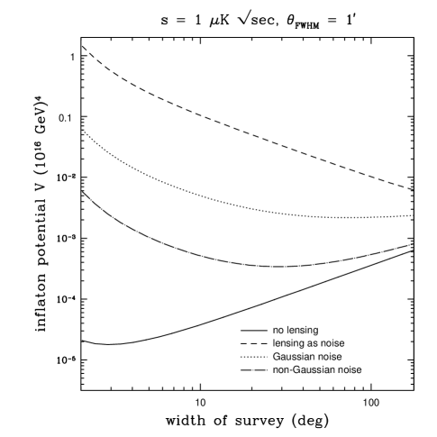
FIG. 7.: Left: Various contributions to the CMB polarization. The long-dashed curve shows the dominant polarization signal in the gradient, or E-mode, component due to scalar perturbations while the solid line shows the curl, or B-mode, polarization signal from the gravitational-wave background assuming an inflationary energy scale of $2.3\times 10^{16}$ GeV, consistent with the limit based on COBE. The short-dashed curve shows the contribution to the B-mode power spectrum due to gravitational lensing. The dotted curve labeled ’G’ is the residual on this contribution due to Gaussian noise when lensing deflections are estimated from a temperature map with a resolution of 1 arcmin, a sensitivity of 1 $\mu$K $\sqrt{\rm sec}$ and a sky coverage of 80%. The dot-dashed curves labeled ’NG’ is the residual if the dominant Gaussian noise is removed as part of this extraction leaving only the non-Gaussian noise of equation (68). Right: Minimum inflation potential observable at $1\sigma$ as a function of survey width for a one-year experiment. The solid curve shows results assuming no lensed E-mode contribution to the B-mode map while the short-dashed curve shows results including the effects of lensing as a noise contribution. The dotted and dot-dashed curves correspond to the lensing subtraction described in the left panel. The order of magnitude improvement in the inflationary energy scales that can be probed confusion-free with CMB polarization data suggests the importance of investigating ways to remove the noise-bias associated with the lensing extraction based on the squared power spectrum.

In general, the CMB data allow high signal-to-noise ratio reconstruction of the lensing effect. We illustrate the extent to which Planck’s frequency cleaned temperature maps can be used as a lensing experiment in figure (6). Here, we show the angular power spectrum of convergence for sources at the last scattering, ie., CMB, and at a redshift of 1; the latter is consistent with what is expected from weak lensing surveys via galaxy ellipticity data. In the right panel, we show the cumulative signal-to-noise ratio for Planck based on the quadratic statistic discussed here and the gradient-based statistic of [14]. The reconstruction based on the squared power spectrum has factor of $\sim$ 3 higher cumulative signal-to-noise than the one based on gradients in the temperature map. This can be understood by noting that the latter method only extracts lensing from the first order expansion of the temperature in terms of the deflection angle, while significant contributions also come from the second order term that is also probed by the proposed estimators.

As shown in figure (6), due to Planck’s beam of $\sim$ 5 to 10 arcmin the reconstruction of convergence becomes noise dominated at multipoles of $\sim$ 1000, while one can probe lensing to much smaller angular scales with galaxy information. The difference between the two curves illustrate the importance of lensing reconstruction for the polarization studies related to gravitational waves. Since CMB photons are affected by potentials out to the last scattering surface, the resulting lensing effect is at least an order of magnitude higher than the lensing effect on sources that are visible from the large scale structure out to a redshift of a few. Thus, it is unlikely that observations of the large scale structure lensing can be used to subtract the lensing contribution to the B-mode polarization sufficiently to permit a confusion free detection of the polarization signal due to gravitational waves. We refer the reader to [16] for a further discussion on this application.

We can extend the discussion in [16] to consider one interesting possibility. As discussed earlier, one can make a significant improvement in the lensing reconstruction when the Gaussian noise bias associated with the temperature squared power spectrum is removed. In such a scenario, the noise contribution associated with the lensing extraction is determined by the non-Gaussianities which are usually an order of magnitude below the dominant Gaussian noise contribution. Such a Gaussian noise bias removal allows an extremely high signal-to-noise extraction of the lensing signal even for experiments with poor sensitivities that are not optimized for the lensing reconstruction. As shown in figure (6), for Planck, the removal of the dominant Gaussian noise leads to detection of the lensing angular power spectrum with a cumulative signal-to-noise ratio of $\sim$ 700, which is roughly a factor of 20 above the level expected when the dominant Gaussian noise contribution is not removed. Such an extraction not only improves the effectiveness of cosmological studies involving lensing of the CMB [37], but also allows a high signal-to-noise separation of the lensed E-mode contribution to the B-mode polarization map of the CMB. This improves the confusion-free limit on the inflationary energy scale attainable with CMB polarization experiments by another order of magnitude [16].

Following [16], we illustrate the importance of noise-bias removal in figure (7). Here, we compare various contributions to the power spectra of CMB polarization, including the lensed E-mode contribution to the B-mode polarization map. We also show the residual lensing contribution to the B-mode map after the lensing effect has been largely removed using an estimator for lensing deflections. The estimator employs a CMB temperature map with a resolution of 1 arcmin and a sensitivity of 1 $\mu$K $\sqrt{\rm sec}$. The curve labeled $NG$ is the residual contribution when the lensing extraction is carried out to the noise level determined by the non-Gaussian noise contribution, assuming that the dominant Gaussian noise contribution can be removed during the lensing extraction. As shown, such a removal provides an order of magnitude improvement over the residual from the dominant Gaussian contribution.

In the right panel of figure (7), we show limits on the inflationary energy scale based on lensing extraction with the remaining residuals depicted in the left panel of the same figure. We refer the reader to [16] for details related to this calculation. For comparison, we also show the inflationary energy scale limit when the lensing contribution is ignored (only instrumental noise) and the limit when the lensing contribution is treated as an additional contribution to the noise associated with the B-mode map. As illustrated in these figures, the potential removal of the Gaussian noise associated with the lensing reconstruction reduces by an order of magnitude the confusion-free upper bound on the gravitational wave signal in the B-mode polarization. Such an improvement motivates the development of practical schemes to remove the noise-bias associated with the dominant Gaussian part of the temperature squared power spectrum. In future work, we will return to this issue and will investigate ways to achieve the required level of noise removal.

VII Summary

We have discussed the four-point correlation function, or the trispectrum in Fourier space, of CMB temperature and polarization anisotropies due to the weak gravitational lensing effect by intervening large scale structure. The trispectrum contains information related to the lensing deflection angle, which for a given configuration of the trispectrum is captured primarily by the diagonal of the quadrilateral that defines the trispectrum in Fourier space. We have devised a statistic involving the power spectrum of squared temperatures that captures this information from the diagonal. This provides an observational approach to extracting the power spectrum of deflection angles induced by the weak gravitational lensing effect on the CMB. The method extends previous suggestions on the use of the squared temperature power spectrum to extract the lensing-secondary correlation power spectrum by probing the bispectrum formed by the lensing effect. The technique presented here is not new and has been discussed previously in the literature by [20]. We extend this work by providing a full derivation of the trispectrum terms both due to lensing and lensing-secondary correlations, and by providing a detailed discussion of the filtering required to minimize the dominant noise component due to Gaussian temperature fluctuations that impairs the extraction of lensing information.

We also extend previous discussions on the trispectrum and associated weak lensing reconstruction from CMB data by calculating in detail contributions to the noise in the reconstruction. Previous work discussed the dominant Gaussian noise, but we include in addition terms associated with non-Gaussian contributions due to lensing alone and the correlation of the lensing effect with other foreground secondary anisotropies in the CMB such as the ISW effect and the SZ effect. When the SZ effect is removed from the temperature maps using its spectral dependence, we find these additional non-Gaussian noise contributions to be an order of magnitude lower than the dominant Gaussian noise. When SZ is not removed, the extraction of lensing information is significantly suppressed; we strongly advise the use of multiple frequencies in upcoming small angular scale CMB experiments, if there is an interest in using data from such experiments to conduct a weak lensing study. The lensing extraction provides a high signal-to-noise ratio detection of the lensing deflection power spectrum. For the Planck surveyor, with frequency-cleaned temperature maps, detection will have a cumulative signal-to-noise of $\sim$ 35, while certain techniques in the literature [14], involving the gradients of the temperature map, only give a cumulative signal-to-noise ratio of $\sim$ 10. Since the extraction with Planck is severely limited by its beam of 5 to 10 arcmin, we strongly recommend higher resolution observations at the arcminute scale. If the noise-bias associated with the dominant Gaussian part of the temperature squared power spectrum is removed, Planck can extract the lensing power spectrum with temperature data alone with a cumulative signal-to-noise ratio around $\sim$ 700. With information from polarization, the signal-to-noise ratio associated with lensing can be further increased by another factor of a few. The order of magnitude improvement in the lensing separation motivates the development of practical methods that can remove the dominant Gaussian noise contribution to the squared temperature power spectrum. In general, our study suggests that future CMB observations can be used as a weak lensing experiment akin to current attempts involving lensing reconstruction from galaxy ellipticity data. This opportunity will help to achieve an ultimate challenge for CMB experiments, a confusion-free direct detection of the gravitational wave signature from inflation.

VIII Appendix I. EE and $\Theta$E estimators

Here we provide the appropriate formulae for deriving optimal filters for the EE and $\Theta$E estimators of $C_{l}^{\phi\phi}$.

A EE estimator

The Fourier transform of the squared E-mode map can be expressed as a convolution of Fourier transforms of the E-mode map itself, analogous to equation (46) of § IV.

$$(EE)({\bf l})=\int\frac{d^{2}{\bf l}_{1}}{(2\pi)^{2}}E({\bf l}_{1})E({\bf l}-{\bf l}_{1})$$ (98)

Defining the power spectrum for the squared E-mode map as $\langle EE({\bf l})EE({\bf l}^{\prime})\rangle=(2\pi)^{2}\delta({\bf l}+{\bf l}^{\prime})C_{l}^{E^{2}E^{2}}$, we write

$$\langle EE({\bf l})EE({\bf l}^{\prime})\rangle=\int\frac{d^{2}{\bf l}_{1}}{(2\pi)^{2}}\int\frac{d^{2}{\bf l}_{2}}{(2\pi)^{2}}\langle E({\bf l}_{1})E({\bf l}-{\bf l}_{1})E({\bf l}_{2})E({\bf l}^{\prime}-{\bf l}_{2})\rangle$$ (99)

As before, this power spectrum will consist of a noise component due to Gaussian fluctuations in the E-mode map and a non-Gaussian contribution due to lensing given respectively by,

$$C_{l}^{E^{2}E^{2}\rm G}=2\int\frac{d^{2}{\bf l}_{1}}{(2\pi)^{2}}C_{l_{1}}^{EE{\rm t}}C_{|{\bf l}-{\bf l}_{1}|}^{EE{\rm t}}\,,$$ (100)

$$C_{l}^{E^{2}E^{2}\rm NG}=C_{l}^{\phi\phi}\left[\int{d^{2}{\bf l}_{1}\over(2\pi)^{2}}\Big{\{}C_{l_{1}}^{EE}{\bf l}\cdot{\bf l}_{1}+C_{|{\bf l}-{\bf l}_{1}|}^{EE}{\bf l}\cdot({\bf l}-{\bf l}_{1})\Big{\}}\cos 2(\varphi_{{\bf l}_{1}}+\varphi_{{\bf l}-{\bf l}_{1}})\right]^{2}$$ (101)

$$+ \int{d^{2}{\bf l}_{1}\over(2\pi)^{2}}\int{d^{2}{\bf l}_{2}\over(2\pi)^{2}}\Big{\{}C_{|{\bf l}_{1}+{\bf l}_{2}|}^{\phi\phi}\left[C_{l_{1}}^{EE}{\bf l}_{1}+C_{l_{2}}^{EE}{\bf l}_{2}\right]\cdot({\bf l}_{1}+{\bf l}_{2})\left[C_{|{\bf l}+{\bf l}_{2}|}^{EE}({\bf l}+{\bf l}_{2})-C_{|{\bf l}-{\bf l}_{1}|}^{EE}({\bf l}-{\bf l}_{1})\right]\cdot({\bf l}_{1}+{\bf l}_{2})$$ (103)

$$\quad\quad\times\cos 2(\varphi_{{\bf l}-{\bf l}_{1}}-\varphi_{{\bf l}+{\bf l}_{2}})\cos 2(\varphi_{{\bf l}_{1}}+\varphi_{{\bf l}_{2}})$$

$$+ C_{|{\bf l}-{\bf l}_{1}+{\bf l}_{2}|}^{\phi\phi}\left[C_{|{\bf l}-{\bf l}_{1}|}^{EE}({\bf l}-{\bf l}_{1})+C_{l_{2}}^{EE}{\bf l}_{2}\right]\cdot({\bf l}-{\bf l}_{1}+{\bf l}_{2})\left[C_{|{\bf l}+{\bf l}_{2}|}^{EE}({\bf l}+{\bf l}_{2})-C_{l_{1}}^{EE}{\bf l}_{1}\right]\cdot({\bf l}-{\bf l}_{1}+{\bf l}_{2})$$ (105)

$$\quad\quad\times\cos 2(\varphi_{{\bf l}_{1}}-\varphi_{{\bf l}+{\bf l}_{2}})\cos 2(\varphi_{{\bf l}-{\bf l}_{1}}+\varphi_{{\bf l}_{2}})\Big{\}}\,.$$

In an analysis similar to that of § IV and § V, we find that the optimal filter in the presence of the Gaussian noise term above is

$$W({\bf l},{\bf l}_{1})=\frac{\left[C_{l_{1}}^{EE}{\bf l}\cdot{\bf l}_{1}+C_{|{\bf l}-{\bf l}_{1}|}^{EE}{\bf l}\cdot({\bf l}-{\bf l}_{1})\right]\cos 2(\varphi_{{\bf l}_{1}}+\varphi_{{\bf l}-{\bf l}_{1}})}{2C_{l_{1}}^{EE{\rm t}}C_{|{\bf l}-{\bf l}_{1}|}^{EE{\rm t}}}\,.$$ (106)

Using this filter, the dominant Gaussian noise $N_{l}$ is given by

$$N_{l}^{-1}=\int{d^{2}{\bf l}_{1}\over(2\pi)^{2}}\frac{\left[C_{l_{1}}^{EE}{\bf l}\cdot{\bf l}_{1}+C_{|{\bf l}-{\bf l}_{1}|}^{EE}{\bf l}\cdot({\bf l}-{\bf l}_{1})\right]^{2}\cos^{2}2(\varphi_{{\bf l}_{1}}+\varphi_{{\bf l}-{\bf l}_{1}})}{2C_{l_{1}}^{EE{\rm t}}C_{|{\bf l}-{\bf l}_{1}|}^{EE{\rm t}}}\,,$$ (107)

while the excess noise due to the additional terms in the E-mode trispectrum is

$$N_{l}^{\rm NG} = N_{l}^{2}\int{d^{2}{\bf l}_{1}\over(2\pi)^{2}}\int{d^{2}{\bf l}_{2}\over(2\pi)^{2}}\Big{\{}W({\bf l},{\bf l}_{1})W(-{\bf l},{\bf l}_{2})$$ (108)

$$\times C_{|{\bf l}_{1}+{\bf l}_{2}|}^{\phi\phi}\left[C_{l_{1}}^{EE}{\bf l}_{1}+C_{l_{2}}^{EE}{\bf l}_{2}\right]\cdot({\bf l}_{1}+{\bf l}_{2})\left[C_{|{\bf l}+{\bf l}_{2}|}^{EE}({\bf l}+{\bf l}_{2})-C_{|{\bf l}-{\bf l}_{1}|}^{EE}({\bf l}-{\bf l}_{1})\right]\cdot({\bf l}_{1}+{\bf l}_{2})$$ (110)

$$\quad\quad\times\cos 2(\varphi_{{\bf l}-{\bf l}_{1}}-\varphi_{{\bf l}+{\bf l}_{2}})\cos 2(\varphi_{{\bf l}_{1}}+\varphi_{{\bf l}_{2}})$$

$$+ C_{|{\bf l}-{\bf l}_{1}+{\bf l}_{2}|}^{\phi\phi}\left[C_{|{\bf l}-{\bf l}_{1}|}^{EE}({\bf l}-{\bf l}_{1})+C_{l_{2}}^{EE}{\bf l}_{2}\right]\cdot({\bf l}-{\bf l}_{1}+{\bf l}_{2})\left[C_{|{\bf l}+{\bf l}_{2}|}^{EE}({\bf l}+{\bf l}_{2})-C_{l_{1}}^{EE}{\bf l}_{1}\right]\cdot({\bf l}-{\bf l}_{1}+{\bf l}_{2})$$ (112)

$$\quad\quad\times\cos 2(\varphi_{{\bf l}_{1}}-\varphi_{{\bf l}+{\bf l}_{2}})\cos 2(\varphi_{{\bf l}-{\bf l}_{1}}+\varphi_{{\bf l}_{2}})\Big{\}}\,.$$

B $\Theta$E estimator

Here we derive the optimal filter and accompanying noise for the $\Theta$E estimator of $C_{l}^{\phi\phi}$. The following equations (113) through (128) for this estimator are entirely analogous to equations (98) through (108) of the preceding subsection of this Appendix. An additional complication here is that, unlike in the $EB$ estimator where $E$ and $B$ are uncorrelated due to parity, $\theta$ and $E$ are correlated with a power spectrum defined by $C_{l}^{\theta E}$ below. This produces an additional term through the lensing effect in addition to that involving correlations between $\theta$ and $E$ separately. First, we expand in Fourier space the product of $\theta$ and $E$ maps,

$$\Theta E({\bf l})=\frac{1}{2}\int\frac{d^{2}{\bf l}_{1}}{(2\pi)^{2}}\left[\Theta({\bf l}_{1})E({\bf l}-{\bf l}_{1})+E({\bf l}_{1})\Theta({\bf l}-{\bf l}_{1})\right]\,,$$ (113)

to obtain

$$\langle\Theta E({\bf l})\Theta E({\bf l}^{\prime})\rangle=\frac{1}{4}\int\frac{d^{2}{\bf l}_{1}}{(2\pi)^{2}}\int\frac{d^{2}{\bf l}_{2}}{(2\pi)^{2}}\langle\left[\Theta({\bf l}_{1})E({\bf l}-{\bf l}_{1})+E({\bf l}_{1})\Theta({\bf l}-{\bf l}_{1})\right]\left[\Theta({\bf l}_{2})E({\bf l}^{\prime}-{\bf l}_{2})+E({\bf l}_{2})\Theta({\bf l}^{\prime}-{\bf l}_{2})\right]\rangle\,,$$ (114)

and

$$C_{l}^{(\Theta E)^{2}\rm G}=\frac{1}{4}\int\frac{d^{2}{\bf l}_{1}}{(2\pi)^{2}}\left[2C_{l_{1}}^{\Theta{\rm t}}C_{|{\bf l}-{\bf l}_{1}|}^{EE{\rm t}}+2C_{l_{1}}^{EE{\rm t}}C_{|{\bf l}-{\bf l}_{1}|}^{\Theta{\rm t}}+4C_{l_{1}}^{\Theta E{\rm t}}C_{|{\bf l}-{\bf l}_{1}|}^{\Theta E{\rm t}}\right]\,.$$ (115)

The non-Gaussian part is

$$C_{l}^{(\Theta E)^{2}\rm NG}=\frac{1}{4}C_{l}^{\phi\phi}\Big{\{}\int{d^{2}{\bf l}_{1}\over(2\pi)^{2}}\left[C_{l_{1}}^{\Theta E}{\bf l}\cdot{\bf l}_{1}+C_{|{\bf l}-{\bf l}_{1}|}^{\Theta E}{\bf l}\cdot({\bf l}-{\bf l}_{1})\right]\left[1+\cos 2(\varphi_{{\bf l}_{1}}+\varphi_{{\bf l}-{\bf l}_{1}})\right]\Big{\}}^{2}$$ (116)

$$+ \frac{1}{4}\int{d^{2}{\bf l}_{1}\over(2\pi)^{2}}\int{d^{2}{\bf l}_{2}\over(2\pi)^{2}}\Big{\{}C_{|{\bf l}_{1}+{\bf l}_{2}|}^{\phi\phi}\Big{\{}\left[C_{l_{1}}^{\Theta}{\bf l}_{1}+C_{l_{2}}^{\Theta}{\bf l}_{2}\right]\cdot({\bf l}_{1}+{\bf l}_{2})\left[C_{|{\bf l}+{\bf l}_{2}|}^{EE}({\bf l}+{\bf l}_{2})-C_{|{\bf l}-{\bf l}_{1}|}^{EE}({\bf l}-{\bf l}_{1})\right]\cdot({\bf l}_{1}+{\bf l}_{2})\cos 2(\varphi_{{\bf l}-{\bf l}_{1}}-\varphi_{{\bf l}+{\bf l}_{2}})$$ (117)

$$+ \left[C_{l_{1}}^{EE}{\bf l}_{1}+C_{l_{2}}^{EE}{\bf l}_{2}\right]\cdot({\bf l}_{1}+{\bf l}_{2})\left[C_{|{\bf l}+{\bf l}_{2}|}^{\Theta}({\bf l}+{\bf l}_{2})-C_{|{\bf l}-{\bf l}_{1}|}^{\Theta}({\bf l}-{\bf l}_{1})\right]\cdot({\bf l}_{1}+{\bf l}_{2})\cos 2(\varphi_{{\bf l}_{1}}+\varphi_{{\bf l}_{2}})$$ (118)

$$+ \left[C_{l_{1}}^{\Theta E}\cos 2(\varphi_{{\bf l}_{1}}+\varphi_{{\bf l}_{2}}){\bf l}_{1}+C_{l_{2}}^{\Theta E}{\bf l}_{2}\right]\cdot({\bf l}_{1}+{\bf l}_{2})\left[C_{|{\bf l}+{\bf l}_{2}|}^{\Theta E}\cos 2(\varphi_{{\bf l}-{\bf l}_{1}}-\varphi_{{\bf l}+{\bf l}_{2}})({\bf l}+{\bf l}_{2})-C_{|{\bf l}-{\bf l}_{1}|}^{\Theta E}({\bf l}-{\bf l}_{1})\right]\cdot({\bf l}_{1}+{\bf l}_{2})$$ (119)

$$+ \left[C_{l_{1}}^{\Theta E}{\bf l}_{1}+C_{l_{2}}^{\Theta E}\cos 2(\varphi_{{\bf l}_{1}}+\varphi_{{\bf l}_{2}}){\bf l}_{2}\right]\cdot({\bf l}_{1}+{\bf l}_{2})\left[C_{|{\bf l}+{\bf l}_{2}|}^{\Theta E}({\bf l}+{\bf l}_{2})-C_{|{\bf l}-{\bf l}_{1}|}^{\Theta E}\cos 2(\varphi_{{\bf l}-{\bf l}_{1}}-\varphi_{{\bf l}+{\bf l}_{2}})({\bf l}-{\bf l}_{1})\right]\cdot({\bf l}_{1}+{\bf l}_{2})\Big{\}}$$ (120)

$$+ C_{|{\bf l}-{\bf l}_{1}+{\bf l}_{2}|}^{\phi\phi}\Big{\{}\left[C_{|{\bf l}-{\bf l}_{1}|}^{\Theta E}({\bf l}-{\bf l}_{1})+C_{l_{2}}^{\Theta E}\cos 2(\varphi_{{\bf l}-{\bf l}_{1}}+\varphi_{{\bf l}_{2}}){\bf l}_{2}\right]\cdot({\bf l}-{\bf l}_{1}+{\bf l}_{2})\left[C_{|{\bf l}+{\bf l}_{2}|}^{\Theta E}({\bf l}+{\bf l}_{2})-C_{l_{1}}^{\Theta E}\cos 2(\varphi_{{\bf l}_{1}}-\varphi_{{\bf l}+{\bf l}_{2}}){\bf l}_{1}\right]\cdot({\bf l}-{\bf l}_{1}+{\bf l}_{2})$$ (121)

$$+ \left[C_{|{\bf l}-{\bf l}_{1}|}^{\Theta E}\cos 2(\varphi_{{\bf l}-{\bf l}_{1}}+\varphi_{{\bf l}_{2}})({\bf l}-{\bf l}_{1})+C_{l_{2}}^{\Theta E}{\bf l}_{2}\right]\cdot({\bf l}-{\bf l}_{1}+{\bf l}_{2})\left[C_{|{\bf l}+{\bf l}_{2}|}^{\Theta E}\cos 2(\varphi_{{\bf l}_{1}}-\varphi_{{\bf l}+{\bf l}_{2}})({\bf l}+{\bf l}_{2})-C_{l_{1}}^{\Theta E}{\bf l}_{1}\right]\cdot({\bf l}-{\bf l}_{1}+{\bf l}_{2})$$ (122)

$$+ \left[C_{|{\bf l}-{\bf l}_{1}|}^{EE}({\bf l}-{\bf l}_{1})+C_{l_{2}}^{EE}{\bf l}_{2}\right]\cdot({\bf l}-{\bf l}_{1}+{\bf l}_{2})\left[C_{|{\bf l}+{\bf l}_{2}|}^{\Theta}({\bf l}+{\bf l}_{2})-C_{l_{1}}^{\Theta}{\bf l}_{1}\right]\cdot({\bf l}-{\bf l}_{1}+{\bf l}_{2})\cos 2(\varphi_{{\bf l}-{\bf l}_{1}}+\varphi_{{\bf l}_{2}})$$ (123)

$$+ \left[C_{|{\bf l}-{\bf l}_{1}|}^{\Theta}({\bf l}-{\bf l}_{1})+C_{l_{2}}^{\Theta}{\bf l}_{2}\right]\cdot({\bf l}-{\bf l}_{1}+{\bf l}_{2})\left[C_{|{\bf l}+{\bf l}_{2}|}^{EE}({\bf l}+{\bf l}_{2})-C_{l_{1}}^{EE}{\bf l}_{1}\right]\cdot({\bf l}-{\bf l}_{1}+{\bf l}_{2})\cos 2(\varphi_{{\bf l}+{\bf l}_{2}}-\varphi_{{\bf l}_{1}})\Big{\}}\Big{\}}\,.$$ (124)

The filter required to suppress the dominant Gaussian noise and extract lensing information is

$$W({\bf l},{\bf l}_{1})=\frac{\left[C_{l_{1}}^{\Theta E}{\bf l}\cdot{\bf l}_{1}+C_{|{\bf l}-{\bf l}_{1}|}^{\Theta E}{\bf l}\cdot({\bf l}-{\bf l}_{1})\right]\left[1+\cos 2(\varphi_{{\bf l}_{1}}+\varphi_{{\bf l}-{\bf l}_{1}})\right]}{C_{l_{1}}^{\Theta{\rm t}}C_{|{\bf l}-{\bf l}_{1}|}^{EE{\rm t}}+C_{l_{1}}^{EE{\rm t}}C_{|{\bf l}-{\bf l}_{1}|}^{\Theta{\rm t}}+2C_{l_{1}}^{\Theta E{\rm t}}C_{|{\bf l}-{\bf l}_{1}|}^{\Theta E{\rm t}}}\,,$$ (126)

and the associated Gaussian noise is

$$N_{l}^{-1}=\int{d^{2}{\bf l}_{1}\over(2\pi)^{2}}\frac{\left[C_{l_{1}}^{\Theta E}{\bf l}\cdot{\bf l}_{1}+C_{|{\bf l}-{\bf l}_{1}|}^{\Theta E}{\bf l}\cdot({\bf l}-{\bf l}_{1})\right]^{2}\left[1+\cos 2(\varphi_{{\bf l}_{1}}+\varphi_{{\bf l}-{\bf l}_{1}})\right]^{2}}{2C_{l_{1}}^{\Theta{\rm t}}C_{|{\bf l}-{\bf l}_{1}|}^{EE{\rm t}}+2C_{l_{1}}^{EE{\rm t}}C_{|{\bf l}-{\bf l}_{1}|}^{\Theta{\rm t}}+4C_{l_{1}}^{\Theta E{\rm t}}C_{|{\bf l}-{\bf l}_{1}|}^{\Theta E{\rm t}}}\,,$$ (127)

while the non-Gaussian noise is

$$C_{l}^{(\Theta E)^{2}\rm NG} = \frac{N_{l}^{2}}{4}\int{d^{2}{\bf l}_{1}\over(2\pi)^{2}}\int{d^{2}{\bf l}_{2}\over(2\pi)^{2}}W({\bf l},{\bf l}_{1})W(-{\bf l},{\bf l}_{2})$$ (128)

$$\times \Big{\{}C_{|{\bf l}_{1}+{\bf l}_{2}|}^{\phi\phi}\Big{\{}\left[C_{l_{1}}^{\Theta}{\bf l}_{1}+C_{l_{2}}^{\Theta}{\bf l}_{2}\right]\cdot({\bf l}_{1}+{\bf l}_{2})\left[C_{|{\bf l}+{\bf l}_{2}|}^{EE}({\bf l}+{\bf l}_{2})-C_{|{\bf l}-{\bf l}_{1}|}^{EE}({\bf l}-{\bf l}_{1})\right]\cdot({\bf l}_{1}+{\bf l}_{2})\cos 2(\varphi_{{\bf l}-{\bf l}_{1}}-\varphi_{{\bf l}+{\bf l}_{2}})$$ (129)

$$+ \left[C_{l_{1}}^{EE}{\bf l}_{1}+C_{l_{2}}^{EE}{\bf l}_{2}\right]\cdot({\bf l}_{1}+{\bf l}_{2})\left[C_{|{\bf l}+{\bf l}_{2}|}^{\Theta}({\bf l}+{\bf l}_{2})-C_{|{\bf l}-{\bf l}_{1}|}^{\Theta}({\bf l}-{\bf l}_{1})\right]\cdot({\bf l}_{1}+{\bf l}_{2})\cos 2(\varphi_{{\bf l}_{1}}+\varphi_{{\bf l}_{2}})$$ (130)

$$+ \left[C_{l_{1}}^{\Theta E}\cos 2(\varphi_{{\bf l}_{1}}+\varphi_{{\bf l}_{2}}){\bf l}_{1}+C_{l_{2}}^{\Theta E}{\bf l}_{2}\right]\cdot({\bf l}_{1}+{\bf l}_{2})\left[C_{|{\bf l}+{\bf l}_{2}|}^{\Theta E}\cos 2(\varphi_{{\bf l}-{\bf l}_{1}}-\varphi_{{\bf l}+{\bf l}_{2}})({\bf l}+{\bf l}_{2})-C_{|{\bf l}-{\bf l}_{1}|}^{\Theta E}({\bf l}-{\bf l}_{1})\right]\cdot({\bf l}_{1}+{\bf l}_{2})$$ (131)

$$+ \left[C_{l_{1}}^{\Theta E}{\bf l}_{1}+C_{l_{2}}^{\Theta E}\cos 2(\varphi_{{\bf l}_{1}}+\varphi_{{\bf l}_{2}}){\bf l}_{2}\right]\cdot({\bf l}_{1}+{\bf l}_{2})\left[C_{|{\bf l}+{\bf l}_{2}|}^{\Theta E}({\bf l}+{\bf l}_{2})-C_{|{\bf l}-{\bf l}_{1}|}^{\Theta E}\cos 2(\varphi_{{\bf l}-{\bf l}_{1}}-\varphi_{{\bf l}+{\bf l}_{2}})({\bf l}-{\bf l}_{1})\right]\cdot({\bf l}_{1}+{\bf l}_{2})\Big{\}}$$ (132)

$$+ C_{|{\bf l}-{\bf l}_{1}+{\bf l}_{2}|}^{\phi\phi}\Big{\{}\left[C_{|{\bf l}-{\bf l}_{1}|}^{\Theta E}({\bf l}-{\bf l}_{1})+C_{l_{2}}^{\Theta E}\cos 2(\varphi_{{\bf l}-{\bf l}_{1}}+\varphi_{{\bf l}_{2}}){\bf l}_{2}\right]\cdot({\bf l}-{\bf l}_{1}+{\bf l}_{2})$$ (134)

$$\quad\quad\times\left[C_{|{\bf l}+{\bf l}_{2}|}^{\Theta E}({\bf l}+{\bf l}_{2})-C_{l_{1}}^{\Theta E}\cos 2(\varphi_{{\bf l}_{1}}-\varphi_{{\bf l}+{\bf l}_{2}}){\bf l}_{1}\right]\cdot({\bf l}-{\bf l}_{1}+{\bf l}_{2})$$

$$+ \left[C_{|{\bf l}-{\bf l}_{1}|}^{\Theta E}\cos 2(\varphi_{{\bf l}-{\bf l}_{1}}+\varphi_{{\bf l}_{2}})({\bf l}-{\bf l}_{1})+C_{l_{2}}^{\Theta E}{\bf l}_{2}\right]\cdot({\bf l}-{\bf l}_{1}+{\bf l}_{2})\left[C_{|{\bf l}+{\bf l}_{2}|}^{\Theta E}\cos 2(\varphi_{{\bf l}_{1}}-\varphi_{{\bf l}+{\bf l}_{2}})({\bf l}+{\bf l}_{2})-C_{l_{1}}^{\Theta E}{\bf l}_{1}\right]\cdot({\bf l}-{\bf l}_{1}+{\bf l}_{2})$$ (135)

$$+ \left[C_{|{\bf l}-{\bf l}_{1}|}^{EE}({\bf l}-{\bf l}_{1})+C_{l_{2}}^{EE}{\bf l}_{2}\right]\cdot({\bf l}-{\bf l}_{1}+{\bf l}_{2})\left[C_{|{\bf l}+{\bf l}_{2}|}^{\Theta}({\bf l}+{\bf l}_{2})-C_{l_{1}}^{\Theta}{\bf l}_{1}\right]\cdot({\bf l}-{\bf l}_{1}+{\bf l}_{2})\cos 2(\varphi_{{\bf l}-{\bf l}_{1}}+\varphi_{{\bf l}_{2}})$$ (136)

$$+ \left[C_{|{\bf l}-{\bf l}_{1}|}^{\Theta}({\bf l}-{\bf l}_{1})+C_{l_{2}}^{\Theta}{\bf l}_{2}\right]\cdot({\bf l}-{\bf l}_{1}+{\bf l}_{2})\left[C_{|{\bf l}+{\bf l}_{2}|}^{EE}({\bf l}+{\bf l}_{2})-C_{l_{1}}^{EE}{\bf l}_{1}\right]\cdot({\bf l}-{\bf l}_{1}+{\bf l}_{2})\cos 2(\varphi_{{\bf l}+{\bf l}_{2}}-\varphi_{{\bf l}_{1}})\Big{\}}\Big{\}}\,.$$ (137)

The trispectrum formed from two temperature and two E-mode terms will contain an additional non-Gaussian contribution through the coupling of the lensing deflection angle to secondary effects. A similar contribution occurs in the temperature trispectrum and was discussed at the end of § III. As in equation (LABEL:eqn:trisec), cumulants such as $\langle\Theta({\bf l})\Theta^{\rm s}({\bf l}^{\prime})\rangle$ will vanish as the secondary effects are decoupled from the primary fluctuations generated at the surface of last scatter. However, contributions come from the correlation between $\Theta^{\rm s}$ and the lensing deflection $\phi$. As before, contributions of equal importance come from both the first and second order terms in $L$ written in equation (25). We consider this additional non-Gaussian contribution for the connected portion of a four-point function in Fourier space

$$\left<\tilde{E}({\mathbf{l}}_{1})\tilde{E}({\mathbf{l}}_{2})\Theta^{\rm t}({\mathbf{l}}_{3})\Theta^{\rm t}({\mathbf{l}}_{4})\right>_{c} = \Big{<}\left(E({{\bf l}_{1}})-\int{d^{2}{\bf l}_{1}^{\prime}\over(2\pi)^{2}}E({{\bf l}_{1}}^{\prime})\cos 2(\varphi_{{\bf l}_{1}^{\prime}}-\varphi_{{\bf l}_{1}})L({{\bf l}_{1}},{{\bf l}_{1}}^{\prime})\right)$$ (140)

$$\quad\left(E({{\bf l}_{2}})-\int{d^{2}{\bf l}_{2}^{\prime}\over(2\pi)^{2}}E({{\bf l}_{2}}^{\prime})\cos 2(\varphi_{{\bf l}_{2}^{\prime}}-\varphi_{{\bf l}_{2}})L({{\bf l}_{2}},{{\bf l}_{2}}^{\prime})\right)\Theta^{\rm s}({{\bf l}_{3}})\Theta^{\rm s}({{\bf l}_{4}})\Big{>}$$

$$= -C_{l_{1}}^{EE}\cos 2(\varphi_{{\bf l}_{1}}+\varphi_{{\bf l}_{2}})\left<L({{\bf l}_{2}},-{{\bf l}_{1}})\Theta^{s}({{\bf l}_{3}})\Theta^{\rm s}({{\bf l}_{4}})\right>-C_{l_{2}}^{EE}\cos 2(\varphi_{{\bf l}_{1}}+\varphi_{{\bf l}_{2}})\left<L({{\bf l}_{1}},-{{\bf l}_{2}})\Theta^{s}({{\bf l}_{3}})\Theta^{\rm s}({{\bf l}_{4}})\right>$$ (142)

$$\quad+\int{d^{2}{\bf l}_{1}^{\prime}\over(2\pi)^{2}}C_{l_{1}^{\prime}}^{EE}\cos 2(\varphi_{{\bf l}_{1}^{\prime}}-\varphi_{{\bf l}_{1}})\cos 2(\varphi_{{\bf l}_{1}^{\prime}}+\varphi_{{\bf l}_{2}})\left<L({{\bf l}_{2}},-{{\bf l}_{1}}^{\prime})L({{\bf l}_{1}},{{\bf l}_{1}}^{\prime})\Theta^{s}({{\bf l}_{3}})\Theta^{\rm s}({{\bf l}_{4}})\right>$$

Contributions to the trispectrum from the first two terms come through the second order term in $L$, with the two $\phi$ terms coupling to $\Theta^{\rm s}$. In the last term, contributions come from the first order term of $L$ similar to the pure lensing contribution to the trispectrum.

After some straightforward simplifications, we can write the connected part of the trispectrum involving lensing-secondary coupling. We symmetrize with respect to the four indices by adding five terms corresponding to the additional permutations of $(l_{1},l_{2},l_{3},l_{4})$ and multiplying by a factor of 1/6.

$$T^{\Theta E{\rm t}}({\mathbf{l}}_{1},{\mathbf{l}}_{2},{\mathbf{l}}_{3},{\mathbf{l}}_{4})=$$ (144)

$$\frac{1}{6}C_{l_{3}}^{\phi{\rm s}}C_{l_{4}}^{\phi{\rm s}}\Big{\{}C^{\Theta}_{l_{1}}\cos 2(\varphi_{{\bf l}_{1}}+\varphi_{{\bf l}_{2}})({{\bf l}_{3}}\cdot{{\bf l}_{1}})({{\bf l}_{4}}\cdot{{\bf l}_{1}})+C^{\Theta}_{l_{2}}\cos 2(\varphi_{{\bf l}_{1}}+\varphi_{{\bf l}_{2}})({{\bf l}_{3}}\cdot{{\bf l}_{2}})({{\bf l}_{4}}\cdot{{\bf l}_{2}})$$ (145)

$$\quad\quad+\left[{{\bf l}_{3}}\cdot({{\bf l}_{1}}+{{\bf l}_{3}})\right]\left[{{\bf l}_{4}}\cdot({{\bf l}_{2}}+{{\bf l}_{4}})\right]C^{\Theta}_{|{\bf l}_{1}+{\bf l}_{3}|}\cos 2(\varphi_{{\bf l}_{1}+{\bf l}_{3}}-\varphi_{{\bf l}_{1}})\cos 2(\varphi_{{\bf l}_{2}+{\bf l}_{4}}-\varphi_{{\bf l}_{2}})$$ (146)

$$\quad\quad+\left[{{\bf l}_{4}}\cdot({{\bf l}_{1}}+{{\bf l}_{4}})\right]\left[{{\bf l}_{3}}\cdot({{\bf l}_{2}}+{{\bf l}_{3}})\right]C^{\Theta}_{|{\bf l}_{1}+{\bf l}_{4}|}\cos 2(\varphi_{{\bf l}_{1}+{\bf l}_{4}}-\varphi_{{\bf l}_{1}})\cos 2(\varphi_{{\bf l}_{2}+{\bf l}_{3}}-\varphi_{{\bf l}_{2}})+\,{\rm Perm.}\Big{\}}$$ (147)

Note that the first two terms come from the first and second term in equation (LABEL:eqn:TEtrisec), while the last two terms are from the third term.

REFERENCES

- [1] P. J. E. Peebles and J. T. Yu, Astrophys. J., 162, 815 (1970); R. A. Sunyaev and Ya.B. Zel’dovich, Astrophys. Space Sci. 7, 3 (1970); J. Silk, Astrophys. J., 151, 459 (1968); see recent review by W. Hu & S. Dodelson, Ann. Rev. Astro. Astrop., in press, astro-ph/0110414 (2001).
- [2] G. Jungman, M. Kamionkowski, A. Kosowsky and D.N. Spergel,Phys. Rev. D, 54 1332 (1995); J.R. Bond, G. Efstathiou and M. Tegmark, MNRAS, 291 L33 (1997); M. Zaldarriaga, D.N. Spergel and U. Seljak, Astrophys. J., 488 1 (1997); D.J. Eisenstein, W. Hu and M. Tegmark, Astrophys. J., 518 2 (1999)
- [3] A. D. Miller et al., Astrophys. J. Lett. 524, L1 (1999); P. de Bernardis et al., Nature 404, 955 (2000); S. Hanany et al., Astrophys. J. Lett. 545, L5 (2000); N. W. Halverson et al., astro-ph/0104489.
- [4] see, for example, review by A. Cooray, 2002, in “2001 Coral Gables Conference: Cosmology and Particle Physics”, eds. B. Kursunoglu & A. Perlmutter; American Institute of Physics Conference Proceedings, astro-ph/0203048
- [5] A. Blanchard and J. Schneider, A&A, 184, 1 (1987); A. Kashlinsky, Astrophys. J., 331, L1 (1988); E. V. Linder, A&A, 206, 1999, (1988); S. Cole and G. Efstathiou, MNRAS, 239, 195 (1989); M. Sasaki, MNRAS, 240, 415 (1989); K. Watanabe and K. Tomita, Astrophys. J., 370, 481 (1991); M. Fukugita, T. Futumase, M. Kasai and E. L. Turner, Astrophys. J., 393, 3 (1992); L. Cayon, E. Martinez-Gonzalez and J. Sanz, Astrophys. J., 413, 10 (1993); U. Seljak, Astrophys. J., 463, 1 (1996)
- [6] D. N. Spergel and D. M. Goldberg, Phys. Rev. D59, 103001 (1999); D. M. Goldberg and D. N. Spergel, Phys. Rev. D, 59, 103002 (1999); A. Cooray and W. Hu, Astrophys. J., 534, 533 (2000). M. Zaldarriaga and U. Seljak, Phys. Rev. D, 59, 123507 (1999); H. V. Peiris and D. N. Spergel, Astrophys. J., 540, 605 (2000).
- [7] F. Bernardeau, A&A, 324, 15 (1997). M. Zaldarriaga, Phys. Rev. D, 62, 063510 (2000).
- [8] W. Hu, Phys. Rev. D, 64, 083005 (2001)
- [9] K. Benabed, F. Bernardeau and L. van Waerbeke, Phys. Rev. D, 63, 043501 (2001); J. Guzik, U. Seljak and M. Zaldarriaga, Phys. Rev. D, 62 043517 (2000);
- [10] R. K. Sachs and A. M. Wolfe, Astrophys. J., 147, 73 (1967).
- [11] R. A. Sunyaev and Ya. B. Zel’dovich, MNRAS, 190, 413 (1980).
- [12] W. Hu, Phys. Rev. D, 62, 043007 (2000).
- [13] A. Cooray, Phys. Rev. D, 65, 063512 (2002).
- [14] U. Seljak & M. Zaldarriaga, Phys. Rev. Lett., 82, 2636 (1999); M. Zaldarriaga and U. Seljak, Phys. Rev. D, 58 023003 (1998).
- [15] A. Cooray, W. Hu and M. Tegmark, Astrophys. J., 540, 1 (2000).
- [16] Kesden, M., Cooray, A., Kamionkowski, M. 2002, PRL submitted, astro-ph/0202434; Knox, L. & Song, Y.-S. 2002, PRL submitted, astro-ph/0202286.
- [17] M. Kamionkowski, A. Kosowsky, and A. Stebbins, Phys. Rev. Lett. 78, 2058 (1997); U. Seljak and M. Zaldarriaga, Phys. Rev. Lett. 78, 2054 (1997).
- [18] M. Zaldarriaga and U. Seljak, Phys. Rev. D 58, 023003 (1998).
- [19] See, for example, M. Kamionkowski and A. Kosowsky, Ann. Rev. Nucl. Part. Sci., 49, 77 (1999).
- [20] W. Hu, Astrophys. J., 557, 79 (2001).
- [21] W. Hu and T. Okamoto, ApJ submitted, astro-ph/0111606 (2001).
- [22] N. Kaiser, Astrophys. J., 388, 286 (1992); N. Kaiser, Astrophys. J., 498, 26 (1998); M. Bartelmann & P. Schneider, Physics Reports in press, astro-ph/9912508 (2000).
- [23] D. Limber, Astrophys. J., 119, 655 (1954).
- [24] J. M. Bardeen Phys. Rev. D22 1882 (1980).
- [25] D. J. Eisenstein & W. Hu, Astrophys. J., 511, 5 (1999).
- [26] E. F. Bunn & M. White, Astrophys. J., 480, 6 (1997).
- [27] P. T. P. Viana & A. R. Liddle, MNRAS, 303, 535 (1999).
- [28] P. J. E. Peebles, The Large-Scale Structure of the Universe, Princeton: Princeton Univ. Press (1980).
- [29] J. A. Peacock and S. J. Dodds MNRAS, 280 L19 (1996).
- [30] Marc Kamionkowski and David N. Spergel, Astrophys. J., 432, 7 (1994).
- [31] P. Valageas, A&A, 354, 767 (2000).
- [32] L. Knox, Phys. Rev. D 52, 4307 (1995).
- [33] A. Cooray, Phys. Rev. D, 64, 043516 (2001).
- [34] U. Seljak & M. Zaldarriaga Astrophys. J., 469, 437 (1996).
- [35] W. Hu, Astrophys. J., 529, 12 (2000).
- [36] J. P. Ostriker and E. T. Vishniac, Astrophys. J., 306, L51 (1986); E. T. Vishniac, Astrophys. J., 322, 597 (1987); S. Dodelson and J. M. Jubas, Astrophys. J., 439, 503 (1995); G. Efstathiou, in Large Scale Motions in the Universe. A Vatican Study Week, ed. V. C. Rubin & G. V. Coyne (Princeton: Princeton University Press), 299 (1988); A. H. Jaffe and M. Kamionkowski, Phys. Rev. D, 58, 043001 (1998);
- [37] Hu, W. Phys. Rev. D, 65, 023003 (2002).