Chaos caused by resonance overlap in the solar neighborhood – Spiral structure at the Bar’s 2:1 outer Lindblad resonance

Abstract

We consider the nature of orbits near the solar neighborhood which are perturbed by local spiral arms and the Milky Way bar. We present a simplified Hamiltonian model which includes resonant terms from both types of perturbations and is similar to the forced pendulum. Via numerical integration of this model we construct Poincare maps to illustrate the nature and stability of the phase space. We find that resonance overlap is most likely to cause widespread chaos when the pattern of the spiral structure puts the solar neighborhood near the 2:1 inner Lindblad resonance (ILR) in the case of a 2-armed pattern, or near the 4:1 ILR in the case of a 4-armed pattern. When this happens both the quasiperiodic orbits which support the spiral structure and those that oscillate with the bar are disrupted near the bar’s 2:1 outer Lindblad resonance (OLR). Consequently the pattern speed of spiral structure which passes through the OLR must be faster than $\sim 0.45$ times the solar neighborhood angular rotation rate if it is 2-armed or faster than $0.75$ times this value if it is 4-armed. Alternatively the OLR may form a boundary between spiral modes at different pattern speeds. In all cases we find that spiral structure is disrupted by the OLR over a narrow range of radius and the extent of the orbits aligned perpendicular to the bar at the OLR is limited by the spiral perturbations. We find that the boundary at an asymmetric drift velocity of $v\sim-30$ km/s of the $u$-anomaly in the velocity distribution in the solar neighborhood is due to the abrupt bifurcation of the orbit families associated with the OLR. The upper boundary at $v\sim-60$ km/s is truncated by the spiral structure. The radial velocity width of the anomaly is probably bounded by chaotic regions which surround the family of quasiperiodic orbits oriented perpendicular to the bar.

1 Introduction

It has been established, beyond doubt, that the Milky is barred as are many nearby galaxies. Evidence for the bar comes from asymmetry in the bulge surface photometry, star counts and interpretation of the gas kinematics (for a recent review see Gerhard 2002). The most common values suggested from these observations are a corotation radius of 3.5-5 kpc and a major axis in-plane angle with respect to the Galactic Center of $\phi_{bar}\sim 15-45^{\circ}$.

The solar neighborhood local velocity distribution is expected to contain structure caused by large scale nearby gravitational perturbations. While structure at low asymmetric drift is likely to be affected by spiral structure and disrupted stellar clusters (e.g., Skuljan et al. 1999), the Hercules stream at a mean heliocentric asymmetric drift velocity of $v\sim 45$km/s is suspected to be related to the 2:1 outer Lindblad resonance (OLR) with the Galactic bar (Dehnen, 1999; Fux, 2001; Raboud et al., 1998). This stream is also known as the $u$-anomaly. Due to the older and rather high metallicity stars in it, the stream probably has a stable kinematic origin (Raboud et al., 1998; Dehnen, 1998). The local velocity distribution as constructed from Hipparcos catalog most clearly shows this stream as a strong and separate feature Dehnen (1998); in fact there is a saddle point in the distribution between the stream and the bulk of the stars at $v\sim 30$ km/s (see Figures in Dehnen 1998; Fux 2001).

Linear theory predicts that the orientation of orbits will shift across the OLR, from oriented along the bar major axis outside the OLR to perpendicular to the bar within it (Binney & Tremaine, 1987). Near the peak of the resonance both types of orbits can exist (Contopoulos, 1975; Weinberg, 1994). Dehnen (2000) showed using a backwards integrating bar growth model that stars were likely to be captured into resonant islands associated with these 2 major orbit families. However the final velocity distribution is strongly dependent upon the timescale over which the bar grows as well as the assumed initial velocity distribution. Fux (2001) considered the stability of orbits and suggested that chaotic regions associated with resonances were likely to cause over-densities in some regions of phase space and under-densities in others. He illustrated with N-body simulations that the resulting stellar distribution could correspond to that observed.

In some sense it is surprising that the OLR with the bar provides such a good explanation for the $u$-anomaly because locally both gaseous and stellar tracers primarily show spiral structure near the solar circle (e.g., Vallée 1995; Drimmel & Spergel 2001). Previous works have not considered the more complicated problem caused by the forces due to local spiral structure in addition to those caused by the bar.

In this paper we consider the dynamics of stars that are affected by perturbations from both spiral structure and the Milky Way bar. We construct a simple Hamiltonian model for the dynamics which contains resonant terms at both the bar pattern speed and a slower pattern speed from local spiral structure. We find that the Hamiltonian can exhibit resonance overlap and so widescale chaos. Consequently we address the issue of orbit stability by computing area preserving or Poincare maps for different values of the spiral pattern speed.

2 Hamiltonian Formalism for the Kinematics

As shown by Contopoulos (1975, 1988), the dynamics of stars confined to the galactic plane moving in a smooth Galactic potential lacking non-axisymmetric perturbations is described by a Hamiltonian which can be written in a third order post epicyclic approximation as

$$H_{0}(I_{1},\theta_{1};I_{2},\theta_{2})=h+\omega_{1}I_{1}+\omega_{2}I_{2}+aI_{1}^{2}+2bI_{1}I_{2}+cI_{2}^{2}...$$ (1)

The high order of the expansion is required to exhibit the bifurcation of the major resonances. The action variables $I_{1}={1\over 2\pi}\int\dot{r}dr$ and $I_{2}=J_{0}-J_{c}$ are integrals of motion when the Hamiltonian is unperturbed. $J_{0}$ is the particle’s angular momentum and $J_{c}$ the angular momentum of a particle in a circular orbit at a radius $r_{c}$ which is the radius of a circular orbit with energy $h$. The frequencies and constants in the above Hamiltonian are evaluated at this radius. We can either to choose to work in a frame rotating with a perturbation pattern or an inertial one. Contopoulos (1975) worked in a frame rotating at the bar or spiral pattern speed, $\Omega_{s}$, so $h\equiv{J_{c}^{2}\over 2r_{c}^{2}}+V_{0}(r_{c})-\Omega_{s}J_{c}$ and $\omega_{2}=\Omega_{c}-\Omega_{s}$ where $\Omega_{c}$ is the angular rotation rate of a circular orbit. Since we will consider more than one perturbation and each perturbation will have a different pattern speed, in this paper we choose to work in an inertial frame. Consequently $h\equiv{J_{c}^{2}\over 2r_{c}^{2}}+V_{0}(r_{c})$ and $\omega_{2}=\Omega_{c}$. In either frame, $J_{c}=r_{c}^{2}\Omega_{c}$ is the angular momentum and $V_{0}(r)$ the axisymmetric component of the potential. The frequency $\omega_{1}=\kappa_{c}$ where $\kappa_{c}$ is the epicyclic frequency which is evaluated at $r_{c}$. Unfortunately the value of $r_{c}$ depends on $\Omega_{s}$ so transferring coordinate systems between an inertial and a rotating one is not trivial.

The constants $a,b,c$ are given in the appendix of Contopoulos (1975). When the rotation curve is flat $\kappa_{c}=\sqrt{2}\Omega_{c}$, $a=-{0.92\over r_{c}^{2}}$, $b=-{1\over\sqrt{2}r_{c}^{2}}$, and $c=-{1\over 2r_{c}^{2}}$.

The radius $r$, the angle $\theta$ and their time derivatives are related to the action angle variables to first order in $I_{1}^{1\over 2}$ (from the appendix of Contopoulos 1975)

$$r-r_{c}\approx\left({2I_{1}\over\kappa_{c}}\right)^{1\over 2}\cos{\theta_{1}}$$ (2)

$${dr\over dt}\approx-(2I_{1}\kappa_{c})^{1\over 2}\sin{\theta_{1}}$$ (3)

$$\theta\approx\theta_{2}-{2\Omega_{c}\over r_{c}\kappa_{c}}\left({2I_{1}\over\kappa_{c}}\right)^{1\over 2}\sin{\theta_{1}}$$ (4)

$$r^{2}{d\theta\over dt}\approx I_{2}+r_{c}^{2}\Omega_{c}$$ (5)

where $\theta_{1}$ is the epicyclic angle and $\theta_{2}$ is the azimuth of the epicyclic center. $\theta_{1}$ and $\theta_{2}$ are the angle variables conjugate to $I_{1}$ and $I_{2}$.

To consider the affect of non-axisymmetric perturbations in the gravitational potential caused by a bar or spiral structure we must estimate the strength of these perturbations in terms of the action angle variables described above. We concentrate on the Lindblad resonances for a number of reasons. They are first order in the amplitude of the perturbation and in ${I_{1}}^{1\over 2}$ and so likely to be strong. The 2:1 OLR from the Galactic bar is near the location of the solar neighborhood. Stars on orbits influenced by the ILRs (inner Lindblad resonances) are required to self consistently support spiral structure (e.g., Contopoulos 1988).

2.1 The perturbation from the Milky Way Bar

For a bar like perturbation we assume that the non-axisymmetric component of the gravitational potential depends on radius and can be expanded in Fourier components

$$V_{1}(r,\theta)=\sum_{m}B_{m}(r)\cos[m(\theta-\Omega_{b}t)]$$ (6)

where $\Omega_{b}$ is the angular rotation rate of the bar. In action angle variables we can write the potential perturbations to first order in $I_{1}^{1/2}$ and the strength of the perturbation (following expressions given by Contopoulos 1988)

$$V_{1,m} (I_{1},\theta_{1};I_{2},\theta_{2})=\left({2I_{1}\over\kappa_{c}}\right)^{1\over 2}\beta_{m}\times~{}~{}~{}~{}~{}~{}~{}~{}~{}~{}~{}~{}~{}~{}~{}~{}~{}~{}~{}~{}$$

$$\left[{\cos(\theta_{1}+m(\theta_{2}-\Omega_{b}t))+\cos(\theta_{1}-m(\theta_{2}-\Omega_{b}t))}\right]$$

where the first and second angular terms correspond to the $m:1$ outer and inner Lindblad resonances respectively. Here

$$\beta_{m}=\left[{{1\over 2}B_{m}^{\prime}+{m\Omega_{c}\over r_{c}\kappa_{c}}B_{m}}\right]$$ (8)

where $B_{m}$ and $B_{m}^{\prime}$ are evaluated at $r_{c}$.

The solar neighborhood is well past the end of the Galactic bar so we can approximate the potential perturbation as a quadrupolar term in the gravitational potential.

$$B_{2}(r)\approx-a_{b}\left({r_{b}\over r}\right)^{3}$$ (9)

where $r_{b}$ is the radius at which the bar ends, $r_{b}\approx 0.45r_{0}$, as found from IR photometry (e.g., Dwek et al. 1995) where $r_{0}$ is the radius of the solar circle from the Galactic Center. The pattern speed of the bar is constrained by to be about 1.85 times the solar neighborhood value of the angular rotation rate, $\Omega_{0}$ (Dehnen, 1999). Fux (2001) considered bars about twice as strong as those considered by Dehnen (1999).

Dehnen (2000) estimates $\alpha={3a_{b}\over v_{c}^{2}}\left({r_{b}\over r_{c}}\right)^{3}\approx 0.01$, so at the solar circle ${a_{b}\over v_{c}^{2}}\sim 0.036.$ From equation (8) and assuming that the rotation curve is flat we find that $\beta_{2}\sim 0.086{a_{b}\over r_{c}}\left({r_{b}\over r_{c}}\right)^{3}$ so at the solar neighborhood we estimate

$$\beta_{2}\sim 0.003{v_{c}^{2}\over r_{c}}$$ (10)

where $v_{c}$ is the velocity of a star in a circular orbit.

2.2 The perturbation from local spiral structure

For spiral structure we assume that the radial variations depend on angle and the amplitude is nearly constant with radius.

$$V_{1,m}(r,\theta)={\rm Re}\left[\sum_{m}A_{m}\exp\left[i(k_{m}r-m(\theta-\Omega_{s}t)+\alpha_{m})\right]\right]$$ (11)

Here $m$ refers to the number of arms, $\Omega_{s}$ to the spiral pattern speed, $k_{m}$ to the wavenumber and $\alpha_{m}$ to an angular offset.

Contopoulos (1975) showed to first order in $I_{1}^{1/2}$ the potential perturbation

$$V_{1,m}(I_{1},\theta_{1};I_{2},\theta_{2})=\left({2I_{1}\over\kappa_{c}}\right)^{1\over 2}\epsilon_{m}\times~{}~{}~{}~{}~{}~{}~{}~{}~{}~{}~{}~{}~{}~{}~{}~{}~{}$$ (12)

$$\left[\cos(\theta_{1}-m(\theta_{2}-\Omega_{s}t+\gamma_{m+}))+\cos(\theta_{1}+m(\theta_{2}-\Omega_{s}t+\gamma_{m-}))\right]$$

where

$$\epsilon_{m} = {A_{m}k_{m}\over 2}\sqrt{1+\left({2m\Omega_{c}\over k_{m}r_{c}\omega_{1}}\right)^{2}}$$ (13)

for ${A_{m}^{\prime}\over kA_{m}}\ll 1$. The angular offsets $\gamma_{m\pm}$ depend on $\alpha_{m}$ and the wavenumber (see Contopoulos 1975 for expressions).

Tracers of spiral structure in the solar neighborhood suggest that the spiral structure is quite tightly wound (e.g., Vallée 1995). In the WKB approximation

$$A_{m}\sim{-2G\Sigma_{0}A\over|k_{m}|}$$ (14)

where $S_{m}$ is the amplitude of the spiral surface density variations divided by the mean surface density (Binney & Tremaine, 1987). For a tightly wound structure we expect that $\epsilon_{m}\sim{A_{m}k_{m}\over 2}$ (taking the largest term in equation 13). The mean surface density of disk mass in the solar solar neighborhood is $\Sigma_{0}\sim 50M_{\odot}{\rm pc}^{-2}$ (Holmberg & Flynn, 2000), and we use $v_{c}\sim 200$km/s. A two armed spiral is seen in the near infrared COBE/DIRBE data with pitch angle in the range $p\sim 15.5^{\circ}$ – $19^{\circ}$ (Drimmel & Spergel, 2001), giving $k_{m}r_{0}=m\cot{p}$ in the range 5.8 – 7.2. The amplitude of the spiral structure could be as large as $S_{m}\sim 0.5-1$ (Drimmel & Spergel, 2001). We estimate for the solar neighborhood

$$A_{m}\sim -0.013v_{c}^{2}S_{m}\left({\Sigma_{0}\over 50M_{\odot}{\rm pc}^{-2}}\right)\left({v_{c}\over 200{\rm km~{}s}^{-1}}\right)^{2}\left({r_{c}\over 8{\rm kpc}}\right)\left({7\over k_{m}r_{c}}\right)$$

$$\epsilon_{m}\sim -0.025{v_{c}^{2}\over r_{c}}S_{m}\left({\Sigma_{0}\over 50M_{\odot}{\rm pc}^{-2}}\right)\left({v_{c}\over 200{\rm km~{}s}^{-1}}\right)^{2}\left({r_{c}\over 8{\rm kpc}}\right).~{}~{}~{}~{}~{}~{}~{}$$ (15)

The expression for $\epsilon_{m}$ is independent of $k_{m}$ and primarily depends on the amplitude of the spiral density variation.

3 Hamiltonian with perturbations from both spiral structure and the Milky Way Bar

We now take the perturbations due to the bar and spiral arms and add them to the unperturbed Hamiltonian. We have estimated the size of the coefficients $\beta$ and $\epsilon$ for these perturbations in the previous section.

We expect that the 2:1 OLR with the Galactic bar and the 2:1 or 4:1 ILR with local spiral structure will be the strongest resonances near the solar neighborhood. So ignoring all other resonant terms we can simplify the problem to

$$H =aI_{1}^{2}+\kappa I_{1}+\Omega I_{2}+\beta_{2}({2I_{1}\over\kappa})^{1\over 2}\cos[\theta_{1}+2(\theta_{2}-\Omega_{b}t)]$$ (16)

$$+\epsilon_{m}({2I_{1}\over\kappa})^{1\over 2}\cos[\theta_{1}-m(\theta_{2}-\Omega_{s}t)-\gamma]+....$$

where $m=2$ for the 2:1 ILR and $m=4$ for the 4:1 ILR. We have assumed that $I_{2}$ is small and so have dropped the terms $bI_{1}I_{2}$ and $cI_{2}^{2}$ from the Hamiltonian.

We do a canonical transformation with generating function

$$F_{2}(J_{1},J_{2},\theta_{1},\theta_{2})=J_{1}(\theta_{1}+2(\theta_{2}-\Omega_{b}t))+J_{2}\theta_{2}$$ (17)

obtaining a resonant angle and new momenta

$$\phi=\theta_{1}+2(\theta_{2}-\Omega_{b}t)$$

$$I_{2}=2J_{1}+J_{2}.$$ (18)

$I_{1}=J_{1}$ and $\theta_{2}$ remain unchanged. Our Hamiltonian becomes

$$H(J_{1},\phi;J_{2},\theta_{2}) =aJ_{1}^{2}+\delta J_{1}+\Omega J_{2}+\beta_{2}({2J_{1}\over\kappa})^{1\over 2}\cos(\phi)$$ (19)

$$+\epsilon_{2}({2J_{1}\over\kappa})^{1\over 2}\cos(\phi+\alpha-\gamma)$$

where

$$\delta=\kappa+2(\Omega-\Omega_{b})$$ (20)

$$\alpha=(m\Omega_{s}+2\Omega_{b})t-(m+2)\theta_{2}.$$ (21)

We can approximate $\theta_{2}\approx\Omega t$ so that $\alpha\approx\nu t$ where

$$\nu=m\Omega_{s}+2\Omega_{b}-(2+m)\Omega.$$ (22)

We rewrite our Hamiltonian in a simpler form

$$H(J_{1},\phi) \approx aJ_{1}^{2}+\delta J_{1}-\beta_{2}({2J_{1}\over\kappa})^{1\over 2}\cos(\phi)$$ (23)

$$-\epsilon_{2}({2J_{1}\over\kappa})^{1\over 2}\cos(\phi+\nu t-\gamma).$$

We rescale by dividing by $a$, put lengths in units of $r_{c}$ and time in units of ${1\over\kappa}$ so that $J_{1}={j_{1}\kappa r_{c}^{2}}$. Since $a<0$ this has the effect of reversing the sign of $t$.

$$h(j_{1},\phi)\approx j_{1}^{2}+\bar{\delta}j_{1}-\bar{\beta}_{2}j_{1}^{1\over 2}\cos(\phi)-\bar{\epsilon}_{2}j_{1}^{1\over 2}\cos(\phi-\bar{\nu}t-\gamma)$$

where the unitless coefficients

$$\bar{\delta} = {\kappa+2(\Omega-\Omega_{b})\over ar_{c}^{2}\kappa}$$ (24)

$$\bar{\beta} = {-\beta_{2}\sqrt{2}\over ar_{c}^{3}\kappa^{2}}$$ (25)

$$\bar{\epsilon} = {-\epsilon_{2}\sqrt{2}\over ar_{c}^{3}\kappa^{2}}$$ (26)

$$\bar{\nu} = {m\Omega_{s}+2\Omega_{b}-(2+m)\Omega\over\kappa}.$$ (27)

If we set $\bar{\epsilon}=0$ then $h=j_{1}^{2}+\bar{\delta}j_{1}-\bar{\beta}j^{1\over 2}\cos{\phi}$. This Hamiltonian is in the same form as $e-e$ resonances discussed in the context of solar system orbital resonances (Murray & Dermott, 1999; Borderies & Goldreich, 1984). As illustrated by Murray & Dermott (1999); Borderies & Goldreich (1984) the resonance bifurcates at a critical value of a parameter which depends on $\bar{\delta}$ and $\bar{\beta}$ (see Figure 1). The resonance has three fixed points when

$${2\bar{\delta}\over 3\bar{\beta}^{2\over 3}}<-1.$$ (28)

One of the fixed points is unstable, the other two correspond to two resonant stable islands of libration at $\phi=0,\pi$. Only one fixed point exists when the above inequality does not hold, and its location is determined by the sign of $\bar{\beta}$. When $\bar{\beta}>0$ this fixed point is at $\phi=0$, otherwise at $\phi=\pi$.

When $\bar{\beta}=0$ the Hamiltonian can be put in the form $h=j_{1}^{2}+(\bar{\delta}-\bar{\nu})j_{1}-\bar{\epsilon}j^{1\over 2}\cos{\phi^{\prime}}$ with a suitable canonical transformation. In this case the bifurcation happens when

$${2(\bar{\delta}-\bar{\nu})\over 3\bar{\epsilon}^{2\over 3}}<-1.$$ (29)

The distinction between regions with two stable fixed points and with one fixed point is important when resonances overlap. For this type of Hamiltonian a separatrix exists only when there are two stable fixed points. Because the period of the orbits becomes infinite at the separatrix, additional perturbations are most likely to cause instability and a chaotic region near the original location of the separatrix. When we have two resonant terms in the Hamiltonian and the resonances overlap, large regions of phase space will become strongly chaotic only when at least one of the resonances contains a separatrix.

Fig. 1.— We plot level contours of the Hamiltonian $H(j,\phi)=j^{2}+j\bar{\delta}-\bar{\beta}j^{1/2}\cos{\phi}$. Dashed contours are negative. The axes are $x,y$ are defined by Eqn(30). The critical value for the resonance to bifurcate happens in the middle panel where ${2\bar{\delta}\over 3\bar{\beta}^{2\over 3}}=-1$. The top of the panel contains a fixed point which would correspond to a closed or periodic orbit aligned with the bar so that $\phi=0$. This is the situation outside the OLR. Inside the OLR the resonance bifurcates, and both periodic orbit families are present. This situation is shown in the bottom panel. The fixed points at $\phi=\pi$ correspond to periodic orbits oriented perpendicular to the bar. Only when ${2\bar{\delta}\over 3\bar{\beta}^{2\over 3}}<-1$ is there a separatrix. Additional perturbations are most likely to cause instability when there is a separatrix.

We now consider the orientations of the orbits and signs of the individual terms. Fixed points in our simple one dimensional system correspond to closed or periodic orbits in the full 2 dimensional system. Assuming that $\Omega_{b}$ is 1.85 times the angular rotation rate at the solar circle (Dehnen, 1999) and a flat rotation curve we estimate $\bar{\delta}\sim 0.2$ at the solar circle. This drops to zero as we approach the 2:1 OLR at a Galactic centric radius of $r\approx 0.9r_{0}$. Because $a\sim-1$, $\bar{\beta}\sim\beta_{2}r_{c}/v_{c}^{2}$ and $\bar{\epsilon}\sim\epsilon r_{c}/v_{c}^{2}$. For radii outside the OLR, $\bar{\delta}>0$ and we expect only one fixed point or periodic orbit. Because $\bar{\beta}>0$ the quasiperiodic orbits at the solar circle, outside the OLR, will be aligned with the bar. They are referred to as the $x_{1}(1)$ orbits (e.g., see Fux 2001; Dehnen 2000). Inside the OLR the resonance bifurcates and two families of periodic orbits (fixed points) exist, the $x_{1}(1)$ and $x_{1}(2)$ families. The $x_{1}(2)$ family is aligned perpendicular to the bar and found at $\phi=\pi$. We expect large scale chaos can occur when there is a separatrix, $\bar{\delta}<0$, and inside the radius of the OLR.

$\Omega_{s}$ is $\sim 0.3$ times the angular rotation rate at the solar circle when $r_{0}$ is just outside the 2:1 ILR and 0.6 if $r_{0}$ is just within the 4:1 ILR. $\gamma$ is related to the phase of the potential for the spiral pattern. and is difficult to constrain from observations. For spiral structure at our location in the solar neighborhood we should be outside the m:1 IRL of the pattern so that $\bar{\delta}-\bar{\nu}<0$. If we aren’t outside the resonance, the stellar orbits will not support the spiral structure, and will negate it instead (e.g., Contopoulos 1988). We expect $\bar{\epsilon}<0$ for periodic orbits with $\phi=\gamma$ to be in phase with the spiral arm. By in phase we mean that the orbit will be aligned with radial maxima on the same axis as the density maxima.

3.1 Generating Poincare maps

Previous works addressing the stability of the orbits in the solar neighborhood have computed Liapunov exponents, studied N-body simulations (Fux, 2001) or carried out backwards integration schemes (Dehnen, 2000). Here we adopt the approach of Fux (2001) and strive to identify regions which regions of phase space that can keep stars for long periods of time. However as we explain below we do this by mapping the nature of phase space instead of computing Liapunov exponents.

The Hamiltonian (Eqn.3) contains two main resonant terms separated by a frequency, $\nu$. This is similar to the forced pendulum. When the two resonances overlap, a chaotic region can be generated at the separatrix of one of the resonances. This zone has a Liapunov time $\sim{2\pi\over\nu}$ (Holman & Murray, 1996). Outside the main chaotic zone we expect quasiperiodic islands. This picture is qualitatively different than that explored by Fux (2001) who illustrated narrow bands of unstable regions, each with different Liapunov timescales. We expect instead large bands of chaos described by one Liapunov time which are surrounding stable islands. Consequently we do not compute Liapunov times for a range of initial conditions but instead map the structure of the phase space itself.

To investigate the stability of the system containing perturbations from both the bar and spiral structure we integrate Eqn(3) numerically. This system is time dependent so the Hamiltonian itself is not conserved. However if we plot points every timestep $P_{\nu}={2\pi\over\nu}$, we derive an area preserving or Poincare map. This procedure generates maps which are like surfaces of section, and these we can use to study the stability of the orbits. In such a map orbits are either area filling or curved loops. We denote area filling orbits as chaotic (in the sense that orbits diverge exponentially) and the curved orbits as quasiperiodic.

This procedure is excellent for addressing the question of orbit stability and identifying the regions accessible to individual orbits. But because we plot every $P_{\nu}$ we cannot tell if an orbit is librating around $\phi$ or around an angle $\phi-\nu t$. This makes it difficult to determine whether fixed points are associated with (or supporting) the bar or the spiral pattern. However we can qualitatively deal with this problem by changing the orientation of the spiral perturbation. We do this by adjusting $\gamma$. We set $\gamma={\pi\over 2}$ so that orbits in phase with the spiral pattern are located at an angle of $\phi\sim{\pi\over 2}$. Orbits perpendicular to the spiral pattern are located at an angle of $-{\pi\over 2}$. In comparison, orbits associated with the bar’s OLR librate about $\phi=0$ or $\pi$.

As is commonly done, (e.g., Murray & Dermott 1999; Borderies & Goldreich 1984), we plot all figures in this paper in a coordinate system with

$$x = \sqrt{2j_{1}}\cos{\phi}$$ (30)

$$y = \sqrt{2j_{1}}\sin{\phi}.$$

With respect to our action variable, $j_{1}={s^{2}/2}$ where $s$ is the radial distance on these plots. Since we defined $J_{1}=j_{1}\kappa r_{c}^{2}$, the epicyclic amplitude is approximately the same as $s$, the radial distance in these plots. In other words $s$ gives the maximum difference between the radial position of a particle and $r_{c}$.

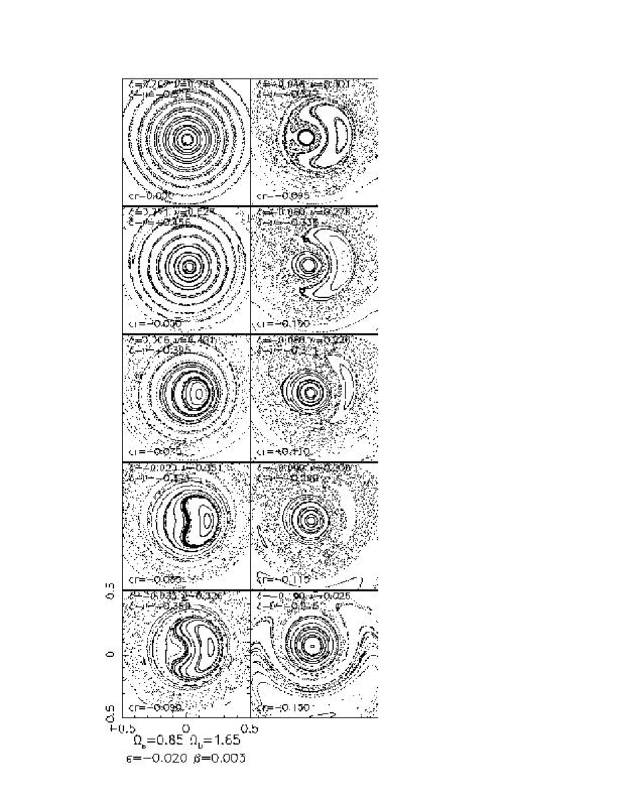
Figure 4: Similar to Figure 2 but we have changed the pattern speed of the spiral structure to $\Omega_{s}=0.85$, with the solar neighborhood outside the 4:1 ILR. For this simulation $m=4$. This system would correspond to a four armed spiral pattern. Phase space as illustrated by this map is similar to that shown in Figure 2.

For each series of integrations (Figures 2–4) we assume a value for $\Omega_{s}$ and $\Omega_{b}$ (in units of the solar neighborhood angular rotation rate $\Omega_{0}$, and $\bar{\epsilon}$ and $\bar{\beta}$ which are directly estimated from the strengths of the spiral structure and bar (see previous sections). We define the radial offset, $dr$, from the radius of the sun as

$$dr={r_{0}-r_{c}\over r_{c}}.$$ (31)

so that ${\Omega_{0}\over\Omega}={r_{c}\over r_{0}}=1+dr$. $\bar{\delta}$ and $\bar{\nu}$ for each integration are calculated from $\Omega_{s}$ and $\Omega_{b}$ assuming a flat rotation curve and for a range of $dr$. In the figures the different panels correspond to different values of $dr$.

Considering the bar only, as we vary $dr$ and so $\delta$, phase space changes in appearance from that shown at the top of Figure 1 to that in the bottom of this figure as we pass through the OLR. Considering the spiral arms only, phase space should look like the bottom of Figure 1 but rotated by 90 degrees since we choose $\gamma=\pi/2$. When $\delta<0$, the bar OLR gains a separatrix which is likely to become unstable when perturbed by the spiral arms.

In Figure 2 we show the result of integrating Eqn.(3) for a 2-armed pattern near the 4:1 ILR of the spiral pattern for moderate spiral and bar strength. For each of 30 particles chosen with different initial conditions, 200 timesteps are plotted with $dt=2\pi/\nu$. For the panel on the top left, corresponding to the Galactic radius of the sun, the orbits librate about $\phi=\pi/2$ and support the spiral structure. At $dr\sim-0.90$, orbits become are aligned with the bar ($x_{1}(1)$ type orbits) and librate about $\phi=0$. At $dr=-0.095$ the $x_{1}(2)$ orbits appear. These librate about $\phi=-\pi$ and are oriented perpendicular to the bar. As $dr$ decreases further the orbits librate closer and closer to $\phi=\pi/2$ and so support the spiral structure and are no longer aligned perpendicular to the bar. For the intermediate region between $dr=-0.10$ and $-0.175$ the quasiperiodic orbits are likely to be oscillating with both the bar and the spiral structure.

Just past the OLR (the center of the resonance is near $\delta=0$, but a separatrix appears only at negative values for $\delta$), we see in Figure 2 that the quasiperiodic regions are bounded by thick bands of area filling or chaotic orbits. The spiral structure is disrupted (unsupported) between $dr=-0.075$ and $-0.115$. Past $dr=-0.175$ the $x_{1}(2)$ orbits are limited by the influence of the spiral structure. In short the spiral structure limits the extent of the orbits perpendicular to the bar OLR and the bar OLR disrupts the spiral structure over a narrow range of radius.

3.2 On the $u,v$ plane

To see if our maps correspond to what is observed in the local velocity distribution we must consider what values of our action angle variables correspond to the $u,v$ velocities that are used to measure stars in the solar neighborhood.

The solar neighborhood velocity distribution is typically plotted with respect to the asymmetric drift velocity (azimuthal), $v$, and the radial velocity, $u$, where $u>0$ corresponds to velocities toward the Galactic center. Orbits at lower $v$ values have lower $r_{c}$ values and are expected to oscillate about galactic radii that are smaller than $r_{0}$, the radius of the solar circle. We now estimate what values of $dr$ correspond to the center and boundary of the Hercules stream or $u$-anomaly.

If we assume a flat rotation curve, the Hamiltonian lacking non-axisymmetric perturbations

$${H\over v_{c}^{2}}={u^{2}\over 2v_{c}^{2}}+{(v_{c}+v)^{2}\over 2v_{c}^{2}}+\ln{r/r_{0}}.$$ (32)

For a circular orbit of radius $r_{c}$ both $u,v=0$ and

$${H\over v_{c}^{2}}=1.0+\ln{r_{c}/r_{0}}.$$ (33)

We set $r=r_{0}$ at the solar neighborhood, equate the two expressions and solve for $r_{c}$ as a function of the asymmetric drift velocity $v$, finding $\ln{r_{c}\over r_{0}}={v\over v_{c}}+{u^{2}+v^{2}\over 2v_{c}^{2}}$. We expand $\ln{r_{c}\over r_{0}}$ and obtain

$$dr={v\over v_{c}}(1+{v\over 2v_{c}})+{u^{2}\over v_{c}^{2}}.$$ (34)

Assuming $u=35$km/s at the center of the stream and $v_{c}=200$km/s

$$dr\sim-0.14~{}~{} ~{}~{}{\rm for}~{}v\sim-30{\rm km~{}s^{-1}}$$ (35)

$$dr\sim-0.18~{}~{} ~{}~{}{\rm for}~{}v\sim-45{\rm km~{}s^{-1}}$$

where $v\sim-45$ km/s at the center of the Hercules stream or $u$-anomaly and $v\sim-30$ km/s at the edge or boundary of the stream.

The stream itself is quite wide along the $u$ direction (over 100 km/s wide) and comparatively quite narrow in the $v$ direction (40 km/s wide). In fact the mean $u$ value of the stream is much less than its $u$ width. If we use a width in $u$ of $35\pm 50$km/s then we estimate a range for $-0.20\lesssim dr\lesssim-0.07$ in the stream.

In Figure 2 we see the $x_{1}(2)$ OLR orbits appear at $dr\sim 0.1$ and not at $dr\sim-0.15$ which is the location of the Hercules stream or $u$-anomaly. We could adjust the pattern speed of the bar to move the resonance over, in fact with $\Omega_{s}=1.95$, we can match the location of the $u$-anomaly. However before we do this we should consider the approximations made in our analysis. In the full Hamiltonian (Eqn.1) there is a term proportional to $I_{1}I_{2}$ which, had we kept it in our analysis, would have caused an additional term ${b\over a}{I_{2}\over\kappa_{c}r_{c}^{2}}$ added to $\bar{\delta}$ in Eqn.(26). In dropping the extra terms in the Hamiltonian we have assumed that $I_{2}$ is small. Because $b$ is the same sign sign as $a$, $\delta$ should be larger than we have calculated. This would have the affect of shifting the location of the resonance to more negative $dr$ or larger distances from the solar neighborhood.

The maps shown in Figures 2–4 do show the likely morphology of phase space near the OLR. However we should not use them to constrain the bar pattern speed at a level better than $25\%$ unless we have taken into account this correction. We estimate the value of the uncertainty from the discrepancy between the pattern speed that we estimate and that constrained by (Dehnen, 1999).

To find out if stars in orbits associated with the $x_{1}(2)$ family can reach the solar neighborhood, we also need to estimate the size of our action variable for the $u$-anomaly. If we assume that $u\sim 0$ then the epicyclic amplitude is set by the condition that we are at $r_{0}$. In other words the maximum value in $r-r_{c}$ is approximately $r_{0}dr$. In terms of the coordinate system of our Poincare maps, a star which reaches the solar neighborhood has $s\sim dr$.

In Figure 2, for $dr\sim-0.10$ the quasiperiodic regions are of size $s\sim 0.15$ which exceeds the value of $dr$. This is large enough that stars in these orbits would reach the solar neighborhood. For $dr\lesssim 0.093$ no $x_{1}(2)$ orbits exist and no stellar orbits aligned perpendicular to the bar will reach the solar neighborhood. Because each value of $dr$ is associated with a $v$ value in the solar neighborhood velocity distribution this implies that above a particular value of $v$ no orbits can be in the quasiperiodic orbit region surrounding the $x_{1}(2)$ periodic orbits. Our model predicts that the $u$-anomaly should have a sharp boundary in $v$ in the solar neighborhood velocity distribution, as observed. A model lacking spiral structure would predict this sharp edge as well since it is determined by the value of $\delta$ at which the resonance bifurcates (see Figure 1).

In Figure 2 we see that past a certain value of $dr$, corresponding to a value of $v$, the quasiperiodic orbits are more likely to be oscillating with the spiral structure than the bar. This implies that there should be an upper boundary in $v$ to the Hercules stream or $u$-anomaly.

We see in Figure 2 that the quasiperiodic orbits oriented perpendicular to the bar are bounded by chaotic regions. This implies that there is a limit in the extent of the epicyclic amplitude of stars associated with this quasiperiodic region. In the solar neighborhood, this implies that there would be a maximum value of $u$ for orbits in the $u$-anomaly. Since stars in the chaotic regions can rapidly achieve very different epicyclic amplitudes, the boundaries of the $u$-anomaly are probably set by the extent of the quasiperiodic orbits associated with the $x_{1}(2)$ orbits.

3.3 Changing the spiral pattern speed

According to Contopoulos (1988); Patsis & Kaufmann (1999), 2-armed spiral structure should only extend between its 2:1 and 4:1 ILRs. These works showed that 2-armed spiral structure was not supported by the stellar orbits past the 4:1 ILR. At first we consider pattern speeds that are faster, and so with the solar neighborhood nearer the 2:1 ILR. The result of integrating Eqn.(3) with a faster pattern, $\Omega_{s}=0.4$, in units of the solar angular rotation rate $\Omega_{0}$ is shown in Figure 3. This pattern speed would be consistent with a 2-armed spiral pattern near its 2:1 ILR.

In Figure 3 we see large scale chaotic regions that completely disrupt the spiral structure and the orbits associated with the bar OLR. Because $\bar{\nu}$ is smaller in this integration than that shown in Figure 2, the resonances are closer together and so more fully overlapped. The scale of the chaotic regions can be reduced by decreasing the strength of the bar and spiral perturbations or the values of $\bar{\epsilon}$, $\bar{\beta}$. However, decreasing both $\bar{\epsilon}$ and $\bar{\beta}$ by a factor of two does not restore the quasiperiodic island about the $x_{1}(2)$ family of periodic orbits. The scale of the chaotic zone is more sensitive to the extent the resonances overlap or to $\bar{\nu}$ which is set by the spiral pattern speed, than to the size of the perturbations. Since we have adopted realistic values for the bar and spiral arm strength we can use this sensitivity to place an approximate limit on the pattern speeds of spiral structure that passes through the bar OLR. We find that the $x_{1}(2)$ are completely disrupted for $\Omega_{s}\lesssim 0.45$ implying that 2-armed spiral structure passing through the OLR is likely to be rotating faster than this.

In Figure 4 we have integrated a spiral pattern at a faster pattern speed of $\Omega_{s}=0.85$ for $m=4$. This would correspond to an 4-armed spiral pattern. The situation is similar to that seen in Figure 2. The OLR bar disrupts the spiral pattern on the outer side of the resonance. The $x_{1}(2)$ orbit family appears abruptly at $dr\sim 0.1$, and the quasiperiodic island oscillates with the bar until $dr\sim 0.12$ where it more strongly supports the spiral structure.

If we reduce the pattern speed of 4-armed spiral structure to $\Omega_{s}<0.75$ phase space looks like that shown in Figure 3. Both the $x_{1}(2)$ orbit family and quasiperiodic orbits that support the spiral structure are destroyed. This implies that 4-armed spiral structure faster than $\Omega_{s}=0.75$ cannot pass through the bar’s OLR.

4 Summary and Discussion

In this paper we consider the dynamics of stars that are affected by perturbations from both spiral structure and the Milky Way bar. We construct a simple one-dimensional Hamiltonian model for the strongest resonances in the epicyclic action and angle variables.

This Hamiltonian is time dependent because the bar and spiral structure in general have different pattern speeds, and resembles a forced pendulum. To address the issue of orbit stability and characterize the nature of phase space in this system we numerically integrate this Hamiltonian. By plotting points only at the period which separates the two resonant perturbations we construct Poincare maps which illustrate where in phase space there are area filling or chaotic orbits instead of quasiperiodic orbits.

The Liapunov time in the chaotic regions is of order the period which separates two resonances. Over much of the resonance this timescale is of order a few times the rotation period. Consequently stars which are located in chaotic regions can move across the region in a few rotation periods. This implies that they can achieve large epicyclic amplitudes and will not remain in any coherent small region in phase space. Streams seen in the local velocity distribution are unlikely to be located in large chaotic regions. In contrast, particles which are located in quasiperiodic regions should maintain their epicyclic amplitudes for much longer times. Our model predicts that the chaotic regions can form large bands. This is a qualitatively different picture than the narrow regions spanning a range of Liapunov times illustrated by Fux (2001) who considered solely perturbations from the bar.

We find that larger spiral pattern speeds $\Omega_{s}$ cause less overlap in the two resonances and so smaller chaotic zones. Spiral structure at a pattern speed which puts the solar circle is near the 2:1 ILR produces extremely large bands of chaos near the 2:1 OLR with the bar. This disrupts the spiral pattern and destroys orbits perpendicular to the bar near the OLR. It is unlikely that 2-armed spiral structure at patterns faster than $\Omega_{s}=0.45$ extends into the OLR. Likewise, it is unlikely that 4-armed spiral faster than $\Omega_{s}=0.85$ extends into the OLR. It is possible that the OLR forms a boundary between spiral structures at different pattern speeds.

2-armed and 4-armed spiral structure at slower pattern speeds are much less disruptive. For a 2-armed pattern with $\Omega_{s}=0.6$, chaotic regions appear near the OLR which disrupt the spiral pattern only across a narrow region. Orbits oriented perpendicular to the bar appear at asymmetric drift velocities and epicyclic amplitudes consistent with existence of quasiperiodic or stable orbits in the local velocity distribution at the Hercules stream or $u$-anomaly. The boundaries of the $u$-anomaly are set by the extent of the quasiperiodic orbits associated with the family of orbits perpendicular to the bar.

In this paper we have considered the combined problem of a resonance from spiral structure and from a Galactic bar. Notably the solar neighborhood contains a wealth of structure at smaller velocities than the $u$-anomaly (Dehnen, 1998). Much of this structure contains old stars and so is likely to be caused by spiral structure. Since there is more than one clump in the distribution it is likely that the solar neighborhood is influenced by spiral structure at more than one pattern speed. Hence we expect complicated phenomena such as that discussed here. In future work we will concentrate on the interplay between different modes of spiral structure.

4.1 Caveats

Our simple Hamiltonian model neglects the coupling between $I_{1}$, the epicyclic action variable and $I_{2}$ which is conjugate to the azimuthal angle and related to the angular momentum. By neglecting this coupling, we have assumed that the particle angular momentum is nearly conserved. Notably in Eqn. 1 the coefficient $b$ is of the same order as $a$, implying that neglecting the $b$ term is only a good approximation when $I_{2}$ is small.

Nevertheless taking the limit of small $I_{2}$ is reasonable first approach and we feel that our simplified model is likely to qualitatively illustrate what happens when multiple resonances are present. We expect that by considering the entire 2-dimensional system other phenomena may be exhibited, for example particles integrated numerically in a system with both spiral structure and a bar can drift in both angular momentum and energy.

2 Fig. 2. – Poincare maps made by integrating the Hamiltonian of Eqn(3) with $m=2$ and with a time step of $2\pi\over\nu$. The panels are at different values of $dr$. The top left panel has the smallest value of $dr$ corresponding to a location near the solar neighborhood. The lower and righter most panel has the most negative value of $dr$ corresponding to a radius closer to the Galactic center. All panels have the same values of $\bar{\epsilon}$, describing the strength of spiral structure, $\Omega_{s}$ the pattern speed of the spiral structure in units of the solar neighborhood angular rotation rate ($\Omega_{0}$), $\bar{\beta}$, describing the strength of the bar, and $\Omega_{b}$, the pattern speed of the bar in units of $\Omega_{0}$. Phase space, as illustrated by the structure in these maps, has two types of orbits; curved linear structures, corresponding quasiperiodic orbits, and area filling orbits corresponding to chaotic regions. The radial distance on these plots is the same as the radial epicyclic amplitude in units of $r_{0}$, or the distance the orbit reaches from $r_{c}$. A dot is placed at the origin for reference. The spiral pattern speed considered here would result from a 2-armed spiral pattern with the solar neighborhood just within the 4:1 ILR.

Fig. 3. – Similar to Figure 2 but we have changed the pattern speed of the spiral structure to $\Omega_{s}=0.4$. This pattern speed could result from a 2-armed spiral pattern with the solar neighborhood fairly near the 2:1 ILR. Since $\nu$ is smaller the resonances are more fully overlapped than is the case for Figure 2. Both the spiral structure and resonant orbits at the OLR are disrupted. A resonant island of $x_{1}(2)$ orbits do not exist for $\Omega_{s}\lesssim 0.45$. The stability of this orbit family is more sensitive on $\nu$ or the spiral pattern pattern speed than the strength of the spiral and bar perturbations.

References

- Binney & Tremaine (1987) Binney, J., & Tremaine, S. 1987, Galactic Dynamics, Princeton University Press, Princeton, NJ
- Borderies & Goldreich (1984) Borderies, N., & Goldreich, P. 1984, Celestial Mechanics, 32, 127
- Contopoulos (1975) Contopoulos, G. 1975, ApJ, 201, 566
- Contopoulos (1988) Contopoulos, G. 1988, A&A, 201, 44
- Dehnen (1998) Dehnen, W. 1998, AJ, 115, 2384
- Dehnen (1999) Dehnen, W. 1999, ApJ, 524, L34
- Dehnen (2000) Dehnen, W. 2000, AJ, 119, 800
- Drimmel & Spergel (2001) Drimmel, R., & Spergel, D. N. 2001, ApJ, 556, 181
- Dwek et al. (1995) Dwek, E. et al. 1995, ApJ, 445, 716
- Fux (2001) Fux, R. 2001, A&A 373, 511
- Gerhard (2002) Gerhard, O. 2002, to appear in: The Dynamics, Structure and History of Galaxies, a conference in honor of Ken Freeman, eds. G.S. Da Costa & E.M. Sadler, ASP Conference Series, (astro-ph/0203109)
- Holman & Murray (1996) Holman, M. J., & Murray, N. W. 1996, AJ, 112, 127
- Holmberg & Flynn (2000) Holmberg, J. & Flynn, C. 2000, 313, 209
- Murray & Dermott (1999) Murray, C. D. & Dermott, S. F. 1999, Solar System Dynamics, Cambridge University Press, Cambridge
- Patsis & Kaufmann (1999) Patsis, P. A., & Kaufmann, D. E. 1999, A&A, 352, 469
- Quillen (2002) Quillen, A. C. (2002), submitted to AJ, astro-ph/0203170
- Raboud et al. (1998) Raboud, D., Grenon, M., Martinet, L., Fux, R., & Udry, S. 1998, A&A, 335, L61
- Skuljan et al. (1999) Skuljan, J., Hearnshaw, J. B., & Cottrell, P. L. 1999, MNRAS, 308, 731
- Taylor & Cordes (1993) Taylor, J. H., & Cordes, J.M. 1993, ApJ 411, 675
- Vallée (1995) Vallée J. P. 1995, ApJ, 454, 119
- Weinberg (1994) Weinberg, M. D. 1994, ApJ, 420, 597