Secular bar formation in galaxies with significant amount of dark matter

Abstract

Using high resolution N-body simulations of stellar disks embedded in cosmologically motivated dark matter halos, we study the evolution of bars and the transfer of angular momentum between halos and bars. We find that dynamical friction results in some transfer of angular momentum to the halo, but the effect is much smaller than previously found in low resolution simulations and is incompatible with early analytical estimates. After 5 Gyrs of evolution the stellar component loses only 5% – 7% of its initial angular momentum.

Mass and force resolutions are crucial for the modeling of bar dynamics. In low resolution (300 – 500 pc) simulations we find that the bar slows down and angular momentum is lost relatively fast. In simulations with millions of particles reaching a resolution of 20-40 pc, the pattern speed may not change over billions of years. Our high resolution models produce bars which are fast rotators, where the ratio of the corotation radius to the bar major semi-axis lies in the range ${\cal R}=1.2-1.7$, marginally compatible with observational results. In contrast to many previous simulations, we find that bars are relatively short. As in many observed cases, the bar major semi-axis is close to the exponential length of the disk.

The transfer of angular momentum between inner and outer parts of the disk plays a very important role in the secular evolution of the disk and the bar. The bar formation increases the exponential length of the disk by a factor of 1.2 -1.5. The transfer substantially increases the stellar mass in the center of the galaxy and decreases the dark matter-to-baryons ratio. As the result, the central 2 kpc region is always strongly dominated by the baryonic component. At intermediate (3 – 10 kpc) scales the disk is sub-dominant. These models demonstrate that the efficiency of angular momentum transfer to the dark matter has been greatly overestimated. More realistic models produce bar structure in striking agreement with observational results.

1 Introduction

Making predictions for the structure of individual galaxies in the framework of cosmological models is a difficult task, that until recently was mostly dominated by modeling of dark matter dominated systems such as dwarf galaxies and low surface brightness galaxies (e.g., Moore, 1994; Flores & Primack, 1994; Kravtsov et al., 1998; van den Bosch & Swaters, 2001; Łokas, 2001; de Blok et al., 2001). It is generally accepted that models do not fare well on those tests predicting too fast rotation in the central region. Excessive amount of dark matter satellites is an additional complication for the cosmological models (Klypin et al., 1999; Moore et al., 1999).

Another layer of problems is on slightly larger scales: luminous parts of normal galaxies and masses in the range of $10^{10}-10^{12}{\rm M}_{{}_{\mathord{\odot}}\;}$. The number of issues is quite large. An excessive amount of dark matter in the bulge may result in too few micro-lensing events (e.g., Zhao & Mao, 1996; Binney & Evans, 2001), but see also (Klypin et al., 2002). Mass modeling of the Milky Way galaxy on different scales is a complicated and quite uncertain issue (e.g., Dehnen & Binney, 1998). For halos predicted by cosmological models the conclusions change from very pessimistic (Navarro & Steinmetz, 2000; Hernández et al., 2001) to neutral (Eke et al., 2001) to more optimistic (Klypin et al., 2002).

One of the contentious issues is the pattern speed of bars. Using analytical arguments and a combination of N-body simulations with rotating solid bars Weinberg (1985); Hernquist & Weinberg (1992) argued that a non-rotating dark matter will exert so much tidal friction that a bar should lose its angular momentum in few rotation periods. For a rigid rotating bar with mass comparable to the mass of the spheroid (including dark matter) inside the bar radius Hernquist & Weinberg (1992) predict that the bar “sheds all its angular momentum typically in less than $\sim 10^{9}$ yr”. If true, that would make impossible for bars to exist in galaxies with dark matter halos. There are no doubts that the dynamical friction operates when a bar rotates inside a dark matter halo. Yet, the rate and the amount of the angular momentum lost by the disk is still a matter of debate. Fully self-consistent N-body simulations with live bars, disks, and dark matter halos (Combes & Sanders, 1981; Sellwood & Athanassoula, 1986; Debattista & Sellwood, 1998, 2000; Athanassoula & Misiriotis, 2002) show that bars slow down far less than what has been predicted by Weinberg (1985); Hernquist & Weinberg (1992). Bars in simulations rotate for billions of years, defying the theoretical expectations. Yet, bars in numerical models are observed to slow down. Debattista & Sellwood (1998, 2000) find that in models, in which initially the dark matter constitutes about the same amount of mass as the stellar disk in the central part of the galaxy, the baryonic component (disk + bar) loses about 40 percent of it angular momentum over $\sim 10$ Gyrs. The bar pattern speed declines by a factor of five after the bar forms. This produces a bar which rotates more than twice slower than the observed bars. The speed of bar rotation is often characterized by the ratio ${\cal R}$ of radius of corotation to the large semi-axis of the bar.

Pattern speeds for real galaxies can be estimated using the method of Tremaine & Weinberg (1984). For a few galaxies – most of them are S0’s – the ratio was measured and is in the range ${\cal R}\approx 1.1-1.7$ (Merrifield & Kuijken, 1995; Gerssen et al., 1999; Aguerri et al., 2003). Bars in models of Debattista & Sellwood (1998, 2000) have ${\cal R}=2.0-2.6$, which contradicts the observed values.

A less known but not less important problem of bars is their length. Combes & Elmegreen (1993) compare lengths of bars in N-body simulations with those observed in galaxies. Even though a good agreement with observations was found, the models either did not include a live halo or included only a bulge component and no halo at all. In more recent simulations with live halos (dark matter dominated or not) the bar semi-major axes are 2-4 times longer than the initial disk exponential length (Debattista & Sellwood, 1998, 2000; Athanassoula & Misiriotis, 2002). These long bars contradict observations because real galaxies typically have bar lengths 0.5-1.5 of the present time exponential disk scale (Elmegreen & Elmegreen, 1985). For example, the bar in our Galaxy is 3-3.5 kpc long (Blitz & Spergel, 1991; Zhao, 1996; Freudenreich, 1998; Gerhard, 2002) which is close to the disk scale length of 2.5-3.5 kpc (Dehnen & Binney, 1998; Hammersley et al., 1999; Gerhard, 2002). In the case of the models studied by Debattista & Sellwood (1998, 2000) the bar extended over the whole disk. That would correspond to 15 kpc, if we scale the models to match our Galaxy. Scaling the dark matter dominated model MH of Athanassoula & Misiriotis (2002) to our Galaxy, the radius of the bar would be 14 kpc (about 4 times the initial exponential length).

The arguments – the slowing down of bars and the lengths of bars – against significant amount of the dark matter in the central parts of normal galaxies have problems on their own. The arguments are based on numerical simulations, which suffer from two types of problems: numerical effects and initial conditions. Numerical resolution is very limited in most simulations. It is often emphasized that models should have a large number of particles to suppress the two-body scattering and to reduce the noise (e.g., Weinberg, 1998; Debattista & Sellwood, 2000). Yet, the force resolution is another important effect, which is often overlooked. For example, the formal (one cell) resolution in simulations of Debattista & Sellwood (2000) was 1/5 of the disk scale length. The scale hight was 1/2 cell, which means that vertical structure was not resolved. If we scale the disk scale length to 3.5 kpc of our Galaxy, then we get the formal resolution of 700 pc. To make the things worse, the real resolution in the Particle Mesh code used by Debattista & Sellwood (2000) is not the formal (cell) resolution, but about twice the formal resolution. For Debattista & Sellwood (1998) and Debattista & Sellwood (2000) simulations this corresponds to 1.4 kpc, which is clearly not enough to mimic the disk of our Galaxy. The resolution in simulations of Fux (1997) was 1.8  kpc at the solar distance.

There are number of reasons why high resolution (both mass and force) is needed for simulations of the bar formation. (1) The central region of galactic models. Propagation of waves through the center and swing amplification are prime suspects for bar instability Toomre (1981); Binney & Tremaine (1987). Simulations must have sufficient resolution to allow correct treatment of these waves. High resolution at the center is also required because during the bar formation the density at the center increases very dramatically (Athanassoula & Misiriotis, 2002, e.g.). This infall of the stellar component to the center should be accurately tracked: the distribution of mass in the central region may affect the structure of the bar (Norman et al., 1996; Berentzen et al., 1998; Shen & Sellwood, 2003). (2) The vertical structure of the disk. Disks of galaxies are very thin - only a couple hundred kpc. Resolving the vertical structure of disks is a challenge for numerical simulations: even optimistically the resolution should be not worse than 100 kpc. Tracking the vertical evolution of the disk is even more difficult than one naively expects. At some stages of the evolution the disk develops waves which oscillate in vertical direction (Fridman & Poliachenko, 1984; Merritt & Sellwood, 1994). Instabilities related with these waves (e.g. the fire-hose instability) are often blamed for sudden thickening of the disk (Raha et al., 1991; Athanassoula & Misiriotis, 2002). In this case the code should be able to maintain both the vertical structure and to treat sufficiently accurately the upward and downward displacements of the thin disk. The vertical oscillations combined with random radial stellar velocities produce coupling of the vertical and the radial directions. As the result, high resolution in the vertical direction must be accompanied with the same resolution in the radial direction. (3) Non linear coupling of waves. The role of interactions between different modes is poorly understood (Contopoulos, 1981; Fridman & Poliachenko, 1984). Theory operates with linear perturbations and typically ignores the nonlinearities (e.g. Nelson & Tremaine, 1999). This does not mean that the nonlinearities are not important: we simply do not know how to handle them analytically. There are no doubts that these effects exist: bars have very large density contrasts. As such, they are nonlinear features. Even more difficult problems are related with the reaction of the dark matter to the small-scale effects in the disk. The dark matter reacts to what happens in the disk sometimes even in a resonant fashion (Athanassoula, 2003). In turn, disk reacts to the disturbances in the halo. This non-linear interaction is clearly important for the long-term evolution of the bar (Athanassoula, 2003). Numerical simulations are the only available tools to study the effects. Coupling of long and short waves (e.g. the short vertical frequencies with long $m=2$ modes) require very high resolution. It should be noted that imposing a high force resolution without adequate mass resolution can be a disaster: simulations would amplify small-scale shot noise potentially leading to incorrect predictions.

Initial setup is questionable in many cases when it comes to the properties of the dark matter halo. If one wants to test predictions of cosmological models, those predictions should be used for setting initial conditions of numerical models. For example, halos predicted by cosmological models are very large and should extend to 200-300 kpc for galaxies of the size of our Galaxy (Klypin et al., 2002). Halos in simulations are much smaller than that. For example, Fux (1997) used halo truncated at 38 kpc. Models of Debattista & Sellwood (2000) were larger - 40 kpc, but still too small as compared to the virial radius of the halo of our Galaxy. The density profile in the outer part of a halo (radii larger 20 kpc for the Milky Way galaxy) should decline as $\rho_{\rm dm}\propto r^{-3}$ (Navarro et al., 1997). This is very different from the profiles used in many simulations of bar formation. For example, Fux (1997) used exponential profile $\rho_{\rm DM}\propto\exp(-r/9.1\,\rm{kpc})$. Athanassoula & Misiriotis (2002) used density profile $\rho\propto\exp(-r^{2}/(35\,\rm{kpc})^{2})/[r^{2}+(1.75\,\rm{kpc})^{2}]$ truncated at 52.5  kpc. Debattista & Sellwood (2000) used polytrops $n=3$, which have little relation with the expected dark matter profile.

The large size and mass of cosmological dark matter halos affect the motion of halo particles even in the central region. Because more massive halos produce deeper potential wells and have larger escape velocities, dark matter particles move faster in the central region. In turn, larger velocities of particles make the halo more resistant to interactions with the stellar disk. Athanassoula (2003) argues that “hotter” halos absorb less angular and result in slower decline of the bar pattern speed.

Both problems of the existing numerical simulations – the resolution and the initial conditions – motivate us to simulate with high resolution models, which use more realistic initial conditions. We use the traditional approach to form a bar: bars are formed by dynamical instability in initially featureless equilibrium disk rotating inside halos (Hohl, 1971; Ostriker & Peebles, 1973; Miller, 1978). In section 2 we describe initial conditions for our models and give details of the code used to run our simulations. The evolution of models is discussed in section 4. In section 5 we present results on the angular momentum of different components. The pattern speed and the structure of bars are presented in section 6. We discuss our results and compare them with the previous results in section 7. A brief summary of our conclusions is given in section 8.

2 Models

2.1 Initial conditions: densities and velocities

We study models, which initially have only two components: an exponential disk and a dark matter halo. No initial bulge or bar are used. Initial conditions for the systems are generated using Hernquist (1993) method. We use the following approximation for the density of the stellar disk in cylindrical coordinates:

$$\rho_{d}(R,z)=\frac{M_{d}}{4\pi z_{0}R_{d}^{2}}e^{-\frac{R}{R_{d}}}sech^{2}(z/z_{0}),$$ (1)

where $M_{d}$ is the mass of the disk, $R_{d}$ is the exponential length, and $z_{0}$ is the scale height. The later was assumed to be constant through the disk. The disk is truncated at five exponential lengths and at three scale heights: $R<5R_{d}$, $z<3z_{0}$. Disk mass was slightly corrected to include the effects of truncation. The vertical velocity dispersion $\sigma_{z}$ is related to the surface stellar density $\Sigma$ and the disk height $z_{0}$:

$$\sigma^{2}_{z}(R)=\pi Gz_{0}\Sigma(R),$$ (2)

where $G$ is the gravitational constant. The radial velocity dispersion $\sigma_{R}$ is also assumed to be directly related to the surface density:

$$\sigma^{2}_{R}(R)=Ae^{-\frac{R}{R_{d}}}.$$ (3)

The normalization constant $A$ in eq. (3) is fixed in such a way that at some reference radius $R_{\rm ref}$ the radial random velocities are $Q$ times the critical value needed to stabilize a differentially rotating disk against local perturbations:

$$\sigma_{R}(R_{\rm ref})=Q\frac{3.36G\Sigma(R_{\rm ref})}{\kappa(R_{\rm ref})},$$ (4)

where $\kappa(R_{\rm ref})$ is the epicycle frequency at the reference radius. The reference radius is chosen to be $R_{\rm ref}=5$ kpc for our models. Results are very insensitive to the particular choice of the reference radius because the stability parameter $Q$ does not change much for radii from $R_{d}$ to few $R_{d}$. We also consider a family of models where $Q$ is fixed along the disk. In this case eq.(4) gives the radial dispersion at every point. The fast increase of the epicycle frequency $\kappa$ in the central region overcomes the exponential growth of density making the disk colder in the centre.

The tangential ($\phi$) component of the rotational velocity and its dispersion are found using the asymmetric drift and the epicyclic approximations:

$$V_{\phi}^{2} = V_{c}^{2}-\sigma_{R}^{2}\left(\frac{2R}{R_{d}}+\frac{\kappa^{2}}{4\Omega^{2}}-1\right),$$ (5)

$$\sigma_{\phi}^{2} = \sigma^{2}_{R}\frac{\kappa^{2}}{4\Omega^{2}}.$$ (6)

Here the circular velocity $V_{c}$ is found as the quadrature sum of the halo and the disk contributions. For the disk component we use the thin-disk approximation.

We assume that the dark matter density profile is described by the NFW profile (Navarro et al., 1997):

$$\rho_{\rm dm}(r) = \frac{\rho_{s}}{x(1+x)^{2}},\ x=r/r_{s},$$ (7)

$$M_{\rm vir} = 4\pi\rho_{s}r^{3}\left[\ln(1+C)-{C\over 1+C}\right],\ C={r_{\rm vir}\over r_{s}},$$ (8)

where $M_{\rm vir}$ and $C$ are the virial mass and the concentration of the halo. For given virial mass the virial radius of the halo is found assuming a flat cosmological model with matter density parameter $\Omega_{0}=0.3$ and the Hubble constant $H_{0}=70\,\rm{km}\,\rm{s}^{-1}{\rm Mpc}^{-1}$.

Knowing the mass distribution of the system $M(r)$, we find the radial velocity dispersion of the dark matter:

$$\sigma_{r,{\rm dm}}^{2}={1\over\rho_{\rm dm}}\int_{r}^{\infty}\rho_{\rm dm}\frac{GM(r)}{r^{2}}dr..$$ (9)

The other two components of the velocity dispersion are equal to $\sigma_{r,{\rm dm}}^{2}$. In other words, the velocity distribution is isotropic, which is a good approximation for the central parts of the dark matter halos (e.g., Colín et al., 2000). Eq.(9) ignores non-spherical deviations of the gravitational acceleration for the dark matter. At each radius we find the escape velocity and remove particles moving faster than the escape velocity.

The dark matter halo is truncated at the virial radius, which for our models is at 250 kpc – 300 kpc radius. During the evolution of the system, the truncation results in a gradual smearing of the outer boundary of the halo. Some particles move to radii larger than the virial radius. They are not replaced by other particles, which, in true equilibrium, would come from the region outside the truncation radius. This creates a rare-faction wave moving inside the halo. The wave never reached the central part of the halo and was always outside the central 100 kpc region.

The distributions eqs. (1-9) are used to produce initial coordinates and velocities of particles. The space is divided into bins. We estimate the expected number of particles inside each bin. We than randomly place specified number of particles inside the bin. Spherical shells are used to initiate dark matter particles. For the disk we use cylindrical shells along radius and equal-spaced bins along the axis of rotation. Velocities are picked from an appropriate Gaussian distribution truncated at the escape velocity. The number of particles was typically 10-20 in each bin. The resulting distribution of particles was tested against expected analytical expressions.

The disks are realized with particles of an equal mass. The dark matter halo is composed of particles of variable mass with small particles placed in the central region and larger particles at larger distances. We double the particle mass as we move further and further from the centre. In total we use 5 mass species with the mass range of 32. The region covered by small mass particles is $\sim 40$ kpc – much larger than the size of the disk. In order to reduce the two-body scattering each dark matter particle in the central region has the same mass as a disk particle.

This procedure is designed to reduce the number of particles and, at the same time, to allow us to cover a very large volume. For example, in model A₁ we have 3.55 million particles inside $\sim 300$ kpc, of which 2.4 million are small particles. We would need 9.5 million particles, if particles of equal mass were used. In the course of evolution some of massive particles come closer to the centre, but their number was always very small.

2.2 Choice of parameters

The approximation eq. (8) formally is valid only for pure dark matter halos without baryons. Contraction of baryons in the process of formation of the disk should significantly affect the dark matter. We try to mimic the effects of the contraction by changing the halo concentration and by tuning parameters of the halo and the disk in such a way that the distribution of the dark matter roughly approximates more realistic models. Klypin et al. (2002) presented such models for the Milky Way and for the M31 galaxies. The models used realistic cosmological dark matter halos and satisfied numerous observational constraints. To some degree we mimic two favored models in that paper: models $A_{1}$ and $B_{1}$, which are described in detail in Klypin et al. (2002).

The first model ($A_{1}$) was designed assuming that the angular momentum of the dark matter was preserved during baryonic collapse. The conservation of angular momentum leads to a specific prediction that in the central $\sim 5$ kpc the density of the dark matter closely follows the density of the baryonic component. The second model ($B_{1}$) includes effects of an exchange of angular momentum between the baryons and the dark matter. The dark matter gains angular momentum through the dynamical friction during early stages of disk and bulge formation, when non-axisymmetric perturbations are expected to be large. Somewhat similar scenario was proposed by El-Zant et al. (2001). Model $B_{1}$ also had significant amount of the dark matter in the central region, but less than in model $A_{1}$. For example, the crossing point, at which the contribution of the dark matter to the circular velocity is equal to that of the baryons, is shifted from 5 kpc in model $A_{1}$ to 12 kpc in model $B_{1}$.

In order to reproduce the effects of the contraction and the exchange of the angular momentum, we increase the concentration of the dark matter halos. Our models have $C=15$ as compared with $C=12$ for models of Klypin et al. (2002). We also adjust parameters of our models (virial mass, exponential length and mass of the disk) to roughly mimic important properties of Klypin et al. (2002) models in the central 20 kpc. For example, our models (A₁ and A₂) have a sub-maximum disk (contributions of the disk and the halo to the circular velocity are approximately equal) at radii $R<5$ kpc with halo dominating at larger radii. The mass of the disk was $4.28\times 10^{10}{\rm M}_{{}_{\mathord{\odot}}\;}$, which is close to the mass of disk+bulge in model $A_{1}$ of Klypin et al. (2002).

The only difference between our two models A₁ and A₂ is in the velocity dispersions of disk particles. For model A₁ we use eq.(3) with the normalization provided by eq.(4) at the reference radius. In the case of model A₂ the eq.(4) is used at all radii (not just at one radius) and the eq.(3) is not used at all. In other words, model A₂ has the same $Q$ parameter at all radii. The main difference between the models is that model A₂ is “colder” in the central region. In the central $\sim 1$ kpc region model A₂ has significantly smaller radial and azimuthal velocity dispersions. Both models have the same circular velocity and the same vertical velocity dispersion.

Our next model (B) has a smaller halo and a more massive disk ($6\times 10^{10}{\rm M}_{{}_{\mathord{\odot}}\;}$). The disk mass is equal to the sum of the disk and the bulge masses in model $B_{1}$ of Klypin et al. (2002). We have a third model called C. This model has a disk mass similar to that in models A, but both radial and vertical scale lengths are shorter. The halo has the same mass as halo in model Bbut concentration is considerable larger.

Parameters of our models are presented in Table 1. Top panels in Figure 1 shows the initial circular velocities $V_{c}=\sqrt{GM(r)/r}$ of the disk and the halo for the models.

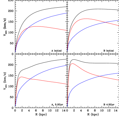
Figure 1: Initial and final circular velocities for model A₁ (left panels) and for model B (right panels). Dashed curves show the contribution of the stellar component $\sqrt{GM(r)/r}$. The dot-dashed curves are for the dark matter. Final models show the total stellar contribution: disk and bar contributions are combined. Initially model A₁ has a sub-maximum disk with the density of the disk being close to the density of the dark matter inside the central 3 kpc region. Model B is more dominated by the disk component: the crossing point of the disk and dark matter is at 9 kpc.

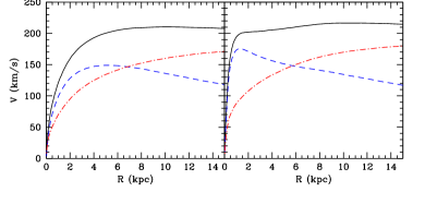
Figure 2: Initial (left panel) and final (right panel) circular velocities for model C. Dashed curves show the contribution of the stellar component $\sqrt{GM(r)/r}$. The full and the dot-dashed curves are for the total circular velocity and for the contribution of the dark matter correspondingly.

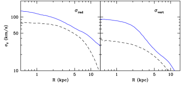
Figure 3: Initial (dashed curves) and final (full curves) rms velocities of the stellar component for the model C. The left panel shows the radial and the right panel shows the vertical ($z$) components of the velocity. Initially the rms velocities are exponential with the ratio of $\sigma_{\rm rad}/\sigma_{\rm vert}\approx 2.5$. Formation of the bar “heats” the vertical component more than the radial one. Outside the bar ($R>5\,\rm{kpc}$) most of the change in the rms velocities occurs in the first 1 Gyr when spiral arms form and dissipate. Notice that in this region the radial and azimutal components of velocities are preferentially heated by the spiral arms.

Table 1: Initial parameters of models

Parameter    $A_{1}\&A_{2}$		B	C
Disk Mass ($10^{10}{\rm M}_{{}_{\mathord{\odot}}\;}$)	$4.28$	$6.0$	$4.8$
Total Mass ($10^{12}{\rm M}_{{}_{\mathord{\odot}}\;}$)	$2.04$	$1.0$	$1.0$
Disk exponential length (kpc)	3.5	3.0	2.9
Disk exponential height (kpc)	0.25	0.25	0.14
Stability parameter $Q$	1.2	1.3	1.2
Halo concentration after	15	15	19
baryonic contraction $C$
Total number of particles ($10^{5}$)	$35.5$	$7.8$	$97.7$
Number of disk particles ($10^{5}$)	$2$	$1.1$	$12.9$
Particle mass ($10^{5}{\rm M}_{{}_{\mathord{\odot}}\;}$)	$2.14$	$5.45$	$0.37$
Maximum resolution (pc)	22	43.6	100.

There are important differences between our models and the models described in Klypin et al. (2002). The later are realistic models, which, in addition to the exponential disk and the halo, have also a nucleus and a triaxial bar. The goal of our paper is to study how a bar develops in an unstable disk. Thus, our models initially do not have either a bar or a bulge: all the stellar mass is in the exponential disk. The bar and the bulge are expected to develop from the disk. Initially, our models mimic to some degree Klypin et al. (2002) models. For example, the exponential disk length is $3-3.5\,\rm{kpc}$. Yet the subsequent evolution of the models was quite significant. Thus, the final parameters a rather different from what was assumed at the beginning. Our final models do not provide a fit to the Milky Way galaxy. Nevertheless, the gross properties (e.g., the maximum circular velocity and the stellar surface density at 8.5 kpc) are not far from what is observed in our Galaxy. This is why we scale different physical quantities to astronomical units (kpc, ${\rm M}_{{}_{\mathord{\odot}}\;}$, and so on).

3 Numerical simulations

3.1 Code

We use the Adaptive-Refinement-Tree (ART) $N$-body code (Kravtsov et al., 1997; Kravtsov, 1999) to run the numerical simulations analyzed in this paper. The code starts with a uniform grid, which covers the whole computational box. This grid defines the lowest (zeroth) level of resolution of the simulation. The standard Particles-Mesh algorithm is used to compute the density and gravitational potential on the zeroth-level mesh with periodical boundary conditions. The code then reaches high force resolution by refining all high density regions using an automated refinement algorithm. The refinements are recursive. A refined region can also be refined. Each subsequent refinement level has half of the previous level’s cell size. This creates a hierarchy of refinement meshes of different resolution, size, and geometry covering regions of interest. Because each individual cubic cell can be refined, the shape of the refinement mesh can be arbitrary and effectively match the geometry of the region of interest. This algorithm is well suited for simulations of a selected region within a large computational box, as in the simulations presented below.

The criterion for refinement is the local density of particles. If the number of particles in a mesh cell (as estimated by the Cloud-In-Cell method) exceeds the level $n_{\rm thresh}$, the cell is split (“refined”) into 8 cells of the next refinement level. The refinement threshold depends on the refinement level. The threshold for cell refinement was low on the zeroth level: $n_{\rm thresh}(0)=2$. Thus, every zeroth-level cell containing two or more particles was refined. The threshold was higher on deeper levels of refinement: $n_{\rm thresh}=3$ and $n_{\rm thresh}=4$ for the first level and higher levels, respectively.

During the integration, spatial refinement is accompanied by temporal refinement. Namely, each level of refinement is integrated with its own time step, which decreases by factor two with each refinement. This variable time stepping is very important for accuracy of the results. As the force resolution increases, more steps are needed to integrate the trajectories accurately.

Figure 4: Test of the code: The growth of the power spectrum of perturbations in the standard cosmological model with $512^{3}$ particles. The dashed curves show the theoretical power spectra at different moments. The full curves show results of the simulation. The wiggles of the simulated spectrum at small wavenumbers $k$ are due to the small number of long-wave harmonics. They should be preserved (shifted upward). From bottom to top the curves are for redshifts $z=48,18.8,9$. At $z=9$ the fluctuations in the simulation have slightly larger amplitude at large wavenumber due to nonlinear effects. The code accurately tracks the growth of about a million of independent harmonics when the amplitude of fluctuations increases many times.

The ART code has the ability to handle particles of different masses. We use multiple masses to increase the mass (and correspondingly the force) resolution inside a region centered around the simulated galaxy.

3.2 Parameters of simulations

The simulations presented here are run using $128^{3}$ zeroth-level grid in a computational box of 2.86 Mpc for models Aand Band 1.4 Mpc for the model C. The models are placed in the center of the grid and far from the periodic images. Because the size of the models are small as compared with the size of the box, the effects of the periodical images are very small and can be neglected. For example, at a distance of 100 kpc from the center of the model Athe contribution of periodic images is less that $7\times 10^{-7}$ of the main galaxy force. Even at 250 kpc, which is close to the virial radius for the models, the tidal force is only $6\times 10^{-5}$ of the force from the central image. Bar formation and evolution are practically unaffected by the periodic boundary conditions.

Model A₁ is simulated for $8.2\times 10^{9}$ yrs with 550 zero-level time steps. The code reaches 10 refinement levels and has about 9 million cells. The number of time steps at the highest resolution level is about 560,000, which gives the time step of $1.5\times 10^{4}$ yrs. With this time step it takes 3500 steps to make one orbital period at the 3 kpc radius. The formal spatial resolution – a cell size at the 10th level – is 22 pc. At about twice that value the force is close to the Newton’s law. Central 6 kpc region was resolved with cells of the size not more than 100 pc. Model A₂ has similar parameters, but it was simulated for 7 Gyrs.

Model B is simulated with a smaller time step of $1.02\times 10^{4}$ yrs (at the 9th level) for $4.5\times 10^{9}$ yrs. It reached the highest resolution of 43.6 pc, but because of fewer particles, the volume with high resolution is significantly smaller than in models A: there are only 3.9 million cells in model B. The number of steps at the highest 9th level is $4.4\times 10^{5}$.

Model C has the largest number of particles: almost 10 million of which more than a million particles belong to the disk. The resolution of this simulation was forced to be not better than 100 pc. Because of large number of particles, the whole disk (up to 14 kpc in radius) is resolved with 100 pc cells. The time step at that resolution was $1.2\times 10^{5}$ yrs. The simulation box was 1.4 Mpc. One of the motivations for the model C is to significantly reduce discreteness effects. For example, our estimate of the two-body scattering time is more than $10^{5}$ Gyrs for this model (see section3.4).

It is interesting to compare our numerical simulations with those presented in Debattista & Sellwood (1998, 2000) and with more recent simulations of Athanassoula & Misiriotis (2002). It is straightforward to compare the resolution of our simulations with that in Debattista & Sellwood (1998, 2000) because we use the same Particle-Mesh algorithm. The formal (one cell) resolution in their simulations was 1/5 of the disk scale length. If we scale the length to 3.5 kpc, than we get the formal resolution of 700 pc, which is 30 times larger than in our models. Athanassoula & Misiriotis (2002) used the TREE code with the Plummer softening of 0.0625 of the disk exponential length. Again, scaling it to 3.5 kpc, we get 220 pc. The force of gravity comes close to the Newton’s law at approximately three Plummer softening lengths or at 660 pc. In our models A this scale is 40-80 pc in the centre and is 200 pc for the entire 6 kpc region.

3.3 Tests of the code

Extensive tests of the code and comparisons with other numerical $N$-body codes can be found in Kravtsov (1999) and Knebe et al. (2000). Kravtsov (1999) (Figure 6) shows the accuracy of the gravitational force. The code was tested against known analytical solutions: (1) the growth of small perturbations in the expanding universe; (2) the spherical accretion (“the Bertschinger solution”); (3) the collapse of a plane wave (the Zeldovich solution). In all tests the code performed extremely well. For example, in the case of the spherical accretion the density at the center should increase by 5 orders of magnitude over tested period of time. The code reproduced that density increase as well as the whole radial density profile. Here we present results of two additional tests, which are more relevant for the bar models: the growth rates of perturbations and the stability of a self-gravitating equilibrium system.

Figure 4 shows the evolution of the power spectrum of perturbations in the standard cosmological model. We use $512^{3}$ particles to set initial conditions at very high redshift $z=50$. The dashed curves in the Figure 4 show the theoretical power spectra at different moments. The full curves show results of the simulation. At the initial moment the deviations of the simulated spectrum from the analytical one at small wave numbers $k$ are due to a small number of long-wave harmonics. This is normal. The code should preserve those deviations at later times, which it clearly does. This test shows that the code is able to accurately follow the evolution of numerous waves over extended period of time during which the waves increase their amplitude many times. For a code this is a very difficult test. It probes every block of the code: gravity solver, motion of particles, and density assignment.There are numerous independent harmonics involved (millions in our case). Each wave must grow independently on others in a well defined way. Because the long waves have much larger amplitude, any erroneous small coupling with short scales would ruin the power spectrum. The code was able to accurately track the growth of all the waves during a period when amplitude of the waves increases many times.

Tests also were performed to check the accuracy and stability of bounded orbits of particles. For example, we set two particles in a circular motion around each other and and run the code with the two particles for hundreds of orbits. We do not find any drift of radius of the orbit. Even a small systematic loss or gain of angular momentum or any adverse effect when a particle moves from one refinement level to another would be clearly detected by the test. The code was tuned not to have any.

We present results of a test of this kind: a long-term stability of an equilibrium self-gravitating configuration. We use 200,000 particles to set an equilibrium halo with the NFW density profile. Three mass species of particles are used, with the second specie being twice as massive as the first one and the third one being four times as massive as the first specie. The halo was truncated at the virial radius of 250 kpc. Parameters of the halo simulation are presented in Table 2. The simulation is then run for 5 Gyrs. There are different goals for this test. Effects of the two-body scattering are discussed in the next section. Here we present the evolution of the density profile. Figure 5 shows the initial and final profiles of the halo. The only observed change in the profile is the decline of the density close to the virial radius. This is caused by the truncation of the configuration at the virial radius. A rarefaction wave gradually moves in to inner parts of the halo. Yet the effect of the wave is very small even at large radii. For example, the density at 100 kpc decline only by 10 percent. The central part ($r<60\,\rm{kpc}$) of the halo does not show any measurable change of the density. Note that the crossing time for the central 2 kpc region is only $10^{7}$yrs for typical velocity 200 $\,\rm{km}\,\rm{s}^{-1}$. Thus, the central part was run for 500 crossing times. The NFW profile is a difficult test because of the large densities and low velocity dispersion in the central region. This cold and dense center potentially is unstable: any numerical errors have a tendency to heat up the center and to reduce its density. The code passes this tough test.

Table 2: Parameters for the test Halo Simulation

Parameter  Model	H1
Halo Mass (${\rm M}_{{}_{\mathord{\odot}}\;}$)	$1\times 10^{12}$
Halo concentration	15
Total number of particles	$2\times 10^{5}$
Total number of mass species	$3$
Formal maximum resolution (pc)	174

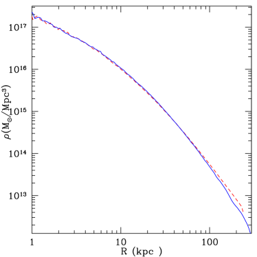
Figure 5: Test of the code: stability of an equilibrium NFW halo modeled with 200,000 particles for 5 Gyrs. The dashed and the full curves show the initial and the final profiles. The central part of the halo is potentially susceptible to different numerical effects and may be affected by the two-body scattering. The profile inside 100 kpc shows no evolution. The slight decline of density outside 100 kpc is due to initial truncation of the halo at virial radius of 250 kpc.

3.4 Two-Body Scattering

Two-body scattering should be very small for systems, which we try to model. Given that our halo and disk are made of particles, every precaution should be made to insure that discreteness does not affect the evolution of the systems. On small scales this is done by imposing a low limit on the number of particles inside a resolution element. The force of gravity becomes Newtonian at about 2 cells. The code is designed to have at least 4 particles in a cells for models A  and B  and about 20 for the model C. Thus, inside one resolution element – a sphere with a radius of 2 cells – there are 130 and 670 particles for models A,B  and C  correspondingly. This large number of particles means that the force acting on a particle can never be dominated by its few closest neighbors. In other words, the code totally eliminates the most damaging close collisions. They cannot possibly happen in the code we use.

Large distance encounters are possible and really happen in our models, but their effect is small. We use the simulation H₁  to investigate the role of the two-body scattering in our numerical experiments and, specifically, to study whether or not angular momentum is affected by this process. The angular momentum for each individual particle should be preserved, if the model is truly collision-less. The change of the orbital angular momentum of any given $i-$th particle, $\Delta L_{i}=|\bf L_{i}-\bf L_{i,\rm init}|$, could be attributed to numerical effects or to the two-body scattering or to a combination of both. If it is dominated by the two-body scattering, the random walk approximation is a reasonable model for the change of orbital angular momentum (Chandrasekhar 1942). In this case the rms value of the change of the orbital angular momentum $\sqrt{\Sigma\Delta L_{i}^{2}/N}$ should grow as the square root of time. The relaxation time associated with the two-body scattering can be defined as the time when the rms change in the orbital angular momentum is comparable to the rms value of the orbital angular momentum $\sqrt{\Sigma L_{i}^{2}/N}$. This could be expressed as:

$$\frac{\Sigma\Delta L_{i}^{2}}{\Sigma L_{i}^{2}}=\frac{t}{T_{Relax}}$$ (10)

The right hand size of eq.(10) is a linear function of $t$ with the slope equal to the inverse of relaxation time ($T_{\rm Relax}$). Figure 6 shows the behavior of $\Sigma\Delta L^{2}/\Sigma(L_{i}^{2})$ over 5 Gyrs. The linear behavior shown in the plot supports the random walk approximation expressed in eq.(10). The slope corresponds to a relaxation time of $3.2\times 10^{3}$ Gyrs. As a test we can compare our result with theoretical estimates. Chandrasekhar (1942, equation 2.380) gives an analytical expression for $T_{\rm Relax}$ due to two-body scattering:

$$T_{\rm Relax}=1.12\times 10^{4}\times\frac{(\sigma_{3D}/20)^{3}}{n_{1}m_{1}m_{2}\log_{10}\Lambda}{\rm Gyrs},$$ (11)

where $m_{1}$ and $m_{2}$ are the mass of the colliding particles in solar masses, $\sigma_{3D}$ is the three dimensional rms velocity of the scattered particles in $\,\rm{km}\,\rm{s}^{-1}$, $n_{1}$ the number density of the scattering particles in $pc^{-3}$ and $\ln\Lambda$ is the Coulomb logarithm. An estimate of $T_{\rm Relax}$ based on a Foker-Planck orbital average, which also uses velocity deviations instead of energies, predicts a coefficient for eq.(11) that differs only by a factor of 0.6. We neglect this small correction. In the case of scattering between particles of the first mass specie (the dominant term) we should use in eq.(11) the mass and the number density of small particles. For the Coulomb logarithm one should take $\ln\Lambda=\ln(b_{\rm max}/b_{\rm min})$, where $b_{\rm max}$ and $b_{\rm min}$ are the maximum and minimum values for the collision impact parameter. A reasonable approximation for these values is: $b_{\rm max}=R_{\rm vir}=252$ kpc and $b_{\rm min}={\rm force~{}resolution}=0.174$ kpc. This gives $\ln\Lambda=7.3$. We calculate the value of the relaxation time using eq.(11). If we take $r=40$ kpc ( 25 % mass radius), $n=1.5\times 10^{-10}pc^{-3}$, $m_{1}=2\times 10^{6}~{}{\rm M}_{{}_{\mathord{\odot}}\;}$, $\sigma_{3D}=171$ km/s, we obtain $T_{\rm Relax}=3.6\times 10^{3}$ Gyrs, which is consistent with the estimate obtained from our halo simulation.

A disk-halo system modeled with particles potentially may experience a large two-body scattering if there is a large difference in masses between particles. This happened in old simulations, when massive halos where modeled with relatively few particles to reduce the computational time. Our main simulations A-C  use 5 mass species, each mass specie being twice massive as the previous one. Thus, the mass ratio of the most massive to the lightest particle is large and equal 16. In the initial configuration the central 40 kpc of the halo and of the disk is sampled only with the particles of the same (small) mass. This setup is designed to minimize the artificial scattering. However, few particles of the 5th (most massive) specie eventually reach the central region. How does this affect the two-body scattering relaxation time estimate? An estimate of the relaxation time $T_{\rm big}$ for particles of the 5-th specie giving energy to (“heating”) the particles of the 1-st mass specie (small particles) can be calculated using eq.(11) by replacing the terms $n_{1}m_{1}m_{2}$ with $n_{b}m_{b}m_{s}$, where indexes $b$ and $s$ refer to big and small particles correspondingly. Thus, the relaxation time of the 1st specie due to scattering with big particles scales as

$$T_{b}=\frac{n_{s}m_{s}}{n_{b}m_{b}}T_{\rm Relax}$$ (12)

Even at late moments of evolution the number density of massive particles in the central 1 kpc is 4 orders of magnitude smaller than the number density of the lightest particles. Using those numbers we obtain that $T_{b}$ is 625 times longer than the relaxation time for the first specie $T_{\rm Relax}$. There is an additional effect, which increases this estimate even more. Eq. (12) does not take into account the fact that large particles move a factor of two faster when they move through the central region as compared with the small particles. This happens because large particles have large energies: initially they are placed at large radii. In other words the two-body relaxation due collisions with big particles is negligible in our simulations.

As an additional test for the effects of the two-body scattering we study how the halo density profile evolves during the simulation: two-body scattering should lead to a gradual decline in the central density for the NFW halo. Figure 5 shows the evolution of the density profile of the halo simulation after 5 Gyrs. The central region of the halo has a higher density and a shorter dynamical time. However we do not find any change in the density profile even after 5 Gyrs. This confirms our estimates of the relaxation time-scale.

The simulation $H_{1}$ is used just as a test for code stability and for estimates of the two-body scattering. Our main simulations have many more particles, and, thus the scattering should be even smaller for them. Using eq. (11) and assuming virial equilibrium we obtain a scaling relation: $T_{\rm Relax}\propto N/\ln N$ (Binney & Tremaine 1987). This relation allows us to scale-up the estimates for the relaxation time based on simulation $H_{1}$ to our simulations with a larger number of particles. For our disk-halo simulations with $3.5\times 10^{6}$ and $10^{7}$ particles we get $T_{\rm Relax}=$ $4.5\times 10^{4}$ Gyrs and $1.2\times 10^{5}$ Gyrs respectively. We can safely ignore any effects of scattering in our disk-halo simulations.

Figure 6: The test of the code for preserving the angular momentum of individual particles. The plot shows the time evolution of the average deviation of the angular momentum $\Delta L_{i}=|\bf L_{i}-\bf L_{i,\rm init}|$ in the $H_{1}$ simulation with $2\times 10^{5}$ particles (crosses). The line is the $\Delta L\propto\sqrt{T}$ fit for the points after 0.5 Gyro. The slope implies the two-body relaxation time $T_{\rm Relax}=3.2\times 10^{3}$ Gyrs, in agreement with the Chandrasekhar formula evaluated at 30 kpc.

3.5 Finding the bar

We follow Debattista & Sellwood (2000) and Athanassoula & Misiriotis (2002) when finding bars in our simulations. We start with finding the centre of the system. This can be done in different ways. Debattista & Sellwood (2000) minimized the sum of distances of all particles relative to a centre. We used a more simple algorithm: the centre of mass of stellar particles. We then bin stellar particles using cylindrical shells spaced equally in logarithm of the distance. For each bin we find the Fourier components of second harmonic of the angular distribution of particles:

$$a_{2}={1\over N}\sum^{N}_{i=1}sin(2\phi_{i}),\quad b_{2}={1\over N}\sum^{N}_{i=1}cos(2\phi_{i}),$$ (13)

where $N$ is the number of stellar particles in the bin and $\phi_{i}$ is the angle of the $i-$th particles. We then find the phase and the amplitude of the second harmonic $A_{2}^{2}=(a_{2}^{2}+b_{2}^{2})/2$.

Except for the very early stages of evolution, when the bar was just emerging, it is easy to identify the bar. In the central region the amplitude of the second harmonic $A_{2}$ changes gradually from bin to bin and its phase $\phi$ is almost constant. At larger distances (typically larger than 5 kpc) the amplitude declines and the phase shows large variations. In the very centre the shot noise complicates the results. Because of these considerations, we use bins with radii in the range 0.5–3 kpc to find the amplitude and the phase of the bars. We find the bar amplitude and its phase as the amplitude-weighted means at different radii: $\langle A_{2}\rangle=\sqrt{\langle A_{2}^{2}\rangle}$, $\langle\phi\rangle=\langle\phi A_{2}\rangle/\langle A_{2}\rangle$. When finding the average amplitude and the phase, we exclude bins with $A_{2}$ less than 1/2 of the maximum amplitude found in the range of the radii. Once the phase of the bar is found at different moments of time, we estimate the frequency of bar rotation (the pattern speed) by numerical differentiation: $\Omega_{p}=d\phi/dt$.

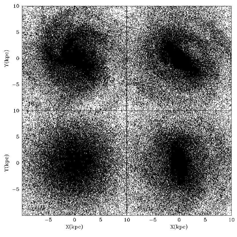
Figure 7: Distribution of the stellar component at different stages of evolution for model A₁. Starting from the left bottom panel in the clock-wise direction the panels correspond to the initial moment; 1 Gyr; 2 Gyr; 3.3 Gyr. The disk rotates counter-clockwise. To avoid crowding we show only every fifth particle. At the distance 5 kpc the disk made 20 orbital periods during 3.3 Gyr.

Finding the radius of the bar is a more difficult problem because bars do not have clear boundaries. Discussion of different methods of finding the bar major axis can be found in Debattista & Sellwood (2000) and in Athanassoula & Misiriotis (2002). We use two different methods, each being sensible and producing reasonable, but slightly different results. We find the surface density along and perpendicular to the bar. We then define the radius of the bar as the radius at which the surface density along the bar is twice of the surface density at the same distance perpendicular to the bar. In the second prescription the bar radius is defined as the radius at which the contours of the surface density have axial ratio of two. We also tried other prescriptions, which are to some degree reminiscent to what was used by Debattista & Sellwood (2000). We find the major semi-axis as the radius at which either the phase of the bar starts to deviate by more than 10 degrees or as the radius at which the amplitude falls below 1/2 of its maximum value. We find that typically the prescriptions based on the surface density give the same results as those based on the amplitude and the phase of the bar. For example, for model A₂ at $t=6.2$ Gyrs the bar radii are: $R_{\rm bar}=4.3\,\rm{kpc}$ ($A_{2,{\rm max}}/2$), $=5.5\,\rm{kpc}$ ($\Delta\phi=10^{\rm o}$), $=4.2\,\rm{kpc}$ ($\Sigma_{\rm major}(r_{\rm major})=2\Sigma_{\rm minor}(r_{\rm major})$), $=5.3\,\rm{kpc}$ ($\Sigma_{\rm major}(r_{\rm major})=\Sigma_{\rm minor}(r_{\rm major}/2)$). Here $\Sigma_{\rm major}(r)$ and $\Sigma_{\rm minor}(r)$ are the stellar surface densities along the major and the minor axes respectively. Nevertheless, we find that the surface densities give more stable results because occasionally spiral waves in the outer disk align with the bar and the amplitude/phase conditions produce spurious results.

We present the total range of the bar sizes produced by the two methods based on the surface density profiles. The estimates vary by 20–30 percent. We would like to emphasize that every estimate was reasonable: the estimates in the middle of the range are no better than the extremes.

4 Evolution

Figure 7 shows the evolution of the stellar component in model A₁. Because the system is relatively hot and the dark matter is significant in the central region, the bar develops slowly. After 1 Gyr (top left panel) the bar has not yet appeared. Nevertheless, extended spiral arms are clearly present in the disk. At that time the system has already made many rotations: at the distance of 5 kpc one orbital period is equal to $T\approx 1.6\times 10^{8}$ yr. The bar develops after 2 Gyrs (top right panel). At that moment its radius is $\approx 4-5$ kpc. The spiral arms can still be seen, but they start to get weaker after that. At the last shown moment (3.3 Gyr) only fragments of spiral arms can be detected. The bar is still very strong, but its amplitude is visibly smaller than at the peak at 1.8 Gyr. The bar gradually grows with time. At later moments (5 – 8 Gyrs) the major semi-axis of the bar is $\approx 6\,\rm{kpc}$. The evolution of model B is qualitatively the same, but it’s initial evolution is more violent and is faster than in the case of model A₁.

The evolution of model A₂ remarkably differs from that of model A₁ in spite of the fact that their initial parameters are almost the same. The only difference between the models is in the initial random stellar velocities: the central part of the disk is colder in model A₂. The initial evolution is faster in model A₂. After 1 Gyr the bar is already in place. The bar is shorter (1 – 1.5 kpc) and it rotates almost twice faster then the bar in model A₁. The bar very slowly increases its length. This slow evolution proceeds for 2 Gyrs. At 3 Gyrs from the beginning the bar suddenly starts to grow in length and its amplitude also increased significantly.

Formation of bars is accompanied by significant redistribution of the stellar mass. Even a visual comparison of the bottom panels in Figure 7 shows that the central surface density increases. Figure 8 shows the evolution of the fraction of stellar mass inside given radius. The total mass inside 5 kpc practically does not change with time. All the mass exchange happens inside the central 1-2 kpc and it is very violent. For example, the stellar mass inside the central 1 kpc region increases by a factor 4 (5.5) after 5 Gyrs (8 Gyrs) of evolution. Note that the time-scale of the initial evolution is about twice shorter in the case of the more disk-dominated model B and for the colder model A₂.

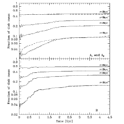
Figure 8: Evolution of fraction of disk mass inside given radius. The top panel is for models A₁ (full curves) and A₂. The bottom panel shows model B. The total mass inside 5 kpc practically does not change with time. Most of the mass exchange happens inside the central 1 – 2 kpc. The disk mass inside the central 1 kpc region increased by a factor 4 by the end of evolution. The time-scale of evolution is about twice shorter in the case of the more disk-dominated model B and the colder model A₂.

Figure 9: The baryon-to-dark matter ratios (bottom panels) and the ratio of the rotational velocity to the velocity dispersion (top panels) for model A₁ (left panels) and model B (right panels). The dash curves show the initial models. The final models are shown with full curves. The central growth of the density goes at the expense of the stellar density in the middle 2 – 8 kpc region. At those radii the final baryon-to-dark matter ratio went down producing dark-matter dominated disk. The top panels show that the heating of the disk preferentially happens in the outer regions outside of the bar. Spiral waves may cause the heating.

Bottom panels in Figure 9 present more detailed information on the change in the densities. In the central 2 kpc the ratio of the stellar density to the dark matter density have increased by a factor of two by the end of the evolution. As the result, even model A₁ became significantly baryon-dominated in the centre, the same effect was already observed in simulations by Athanassoula & Misiriotis (2002). The Figure also shows that the central growth of the density goes at the expense of the stellar density in the middle part ( 2–8 kpc ). At those radii the final baryon-to-dark matter ratio was a bit surprising: it went down producing a dark-matter dominated disk. This effect is more pronounced in model B, which was initially more baryon-dominated than models A.

The dramatic changes of the disk component hardly affect the dark matter: it stays almost unchanged. There is a 20 (40) per cent increase of the dark matter density in the central 2 kpc region after 5 (8) Gyrs of evolution . The rest of the halo is practically unaffected in agreement with Athanassoula & Misiriotis (2002).

Because of the violent processes in the central region, one would naively expect to find a very strong heating of the disk in the central part and much less in the outer parts. The ratio of the rotational velocity $V_{\phi}$ to the velocity dispersion $\sigma_{\phi}$ characterizes the “hotness” of disk. The top plots in the Figure 9 show just an opposite trend: the heating is relatively stronger in the outer part of the disk. A possible explanation for this is the heating by spiral waves that appeared in the outer parts of the disk. Large amplitude spiral waves produce non-circular motions and increase the azimuthal dispersion. After the waves die out, they leave behind a hotter disk.

5 Angular momentum

Formation of a bar is accompanied and even may be driven by the exchange of angular momentum between different components of the system. The exchange of angular momentum between the quickly rotating stellar component and the non-rotating dark matter is of special interest because is often used as one of the arguments against the presence of a significant amount of the dark matter in the central parts of galaxies. Numerically it is a challenge to simulate the two-component system: any artificial numerical coupling will result in a transfer of some angular momentum from the stellar to the dark matter component. For an axisymmetric system no transfer should happen. Once the bar or any other non-axisymmetric perturbation is formed, the dark matter should react to it by generating a wake behind the perturbation, which must result in a transfer of the angular momentum to the dark matter. The exchange of the angular momentum is not limited by the disk-dark matter interaction. The stellar component also experiences the exchange between different parts of the disk, which we find to be much more important for the evolution and for the structure of bars.

Figure 10 presents the evolution of the z-component of the angular momentum of the stellar component (disk + bar; top panels), the pattern speed of bars (middle panels), and the bar amplitudes (bottom panels) for all the models. Figure 11 shows details of the evolution of the angular momentum for A₁ and B models. The total stellar angular momentum clearly is declining with time, but the rate of the decline is very small. After 5 Gyrs the change was $\approx 5$% for all the models. The disk of the model A₁ lost 13 per cent of the angular momentum after 8 Gyrs of evolution. This level of the angular momentum loss is at odds with the results of Debattista & Sellwood (2000), who find about 40% decline. A large fraction of the angular momentum loss in the model A₁ happened during a short period (5-6 Gyrs after the start), when the bar was increasing its amplitude. When the growth abruptly stopped at $t\approx 6$ Gyrs, the rate of the decline also slowed down dramatically.

It was interesting to find that the specific angular momentum $L_{z}$ at different radii in Figure 11 shows very little evolution. Only at the very centre the angular momentum declines slightly. At larger radii the specific angular momentum is practically constant. At first sight this indicates that the distribution of the angular momentum does not evolve. This is not true. Figure 8 shows that the stellar mass in the central region increases quite substantially. Because the specific angular momentum $L_{z}(r)$ at a given radius does not change, this mass increase implies that the stellar particles that accumulate in the central region, actually lose their angular momentum. This is clarified by Figure 12 that shows significant changes in the distribution of the angular momentum of the stellar particles in the course of the evolution. The changes are especially noticeable at low $L_{z}$: a large peak forms. The peak at very low (almost zero) angular momentum is made of the particles located in the central region. The particles initially had intermediate angular momentum and lost some of it during the bar formation. As the result of this migration of particles the distribution of $L_{z}$ at later moments has a deep at intermediate angular momenta. The number of particles at large $L_{z}$ also increases, which is more clearly seen in the case of model B.

Evolution of the $L_{z}$ distribution is not gradual. Most of the changes occur before and during the bar formation. Model B clearly shows that once the bar has formed (after 1 Gyr of evolution) the distribution experiences very little evolution. This indicates that the bar itself does not lead to a significant exchange of the angular momentum between the particles. Most of the evolution is done not by the bar, but by the processes that produce the bar. Nevertheless, the evolution does not stop after the bar forms. It proceeds, but with a much lower rate.

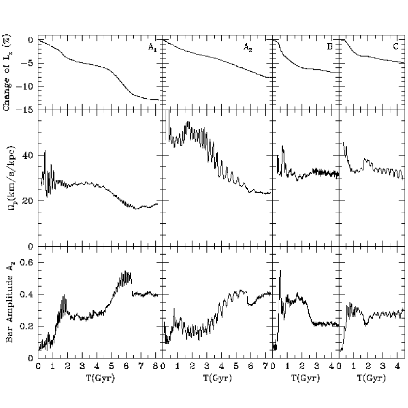
Figure 10: Evolution of the bar amplitude (bottom panels), the pattern speed (middle panels), and disk angular momentum for the models A₁ (left column of panels), A₂ (middle column of panels) and B (right column). In all cases the angular momentum declines due to the dynamical friction with the dark matter. The decline is very small - only few percent for $\sim 5$ Gyrs of evolution. Note the complex behavior of bar amplitude and its correlation with the pattern speed. The pattern speed remains almost constant during periods, when the bar amplitude does not evolve (e.g., $t=2-5$ Gyrs for model A₁or $t=5-7$ Gyrs for model A₂). Periods of fast increase of the bar amplitude correlate with the decline of the pattern speed (e.g.,$t=3-5$ Gyrs for model A₂).

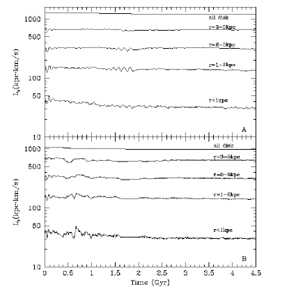
Figure 11: Evolution of the specific angular momentum of the disk for the A₁ (top panel) and the B (bottom panel) models. The top curves in each panel show that the total angular momentum of disk particles declines very little – few per cent after 4.5 Gyrs of evolution. The other curves present an average specific angular momentum for disk particles inside spherical shells indicated in the plot. Only the very central region (radius less than 1 kpc) exhibits some decrease (a factor of 1.5) of angular momentum. Outside the very centre the specific angular momentum does not change.

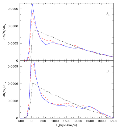
Figure 12: Distribution of the z-component of the angular momentum of the stellar particles for models A₁ (top panel) and B (bottom panel) at different moments of time. Initial distribution is shown by dot-dashed curves. Particles with low angular momentum are preferentially at small radii. Large angular momentum is coming from particles at large distances. Dashed curves are for 1-1.5 Gyrs after the beginning of the evolution. The final distribution (full curves, 4.5-5 Gyrs) is qualitatively the same for both models. The peak at small angular momenta corresponds to the bar. The number of particles with intermediate angular momenta substantially decreases during the evolution. There is an excess of particles with very large angular momentum. The changes in the distribution are much stronger in the case of model B, which has less dark matter and has a more massive disk.

Because of the large moment of inertia of the dark matter, it is difficult to detect small changes in the distribution of the angular momentum of the dark matter particles. The largest effect was found in the central region. By the end of the evolution the dark matter in the central 2 kpc region rotated with velocity 3 – 7 $\,\rm{km}\,\rm{s}^{-1}$. This rotation has very little dynamical effect. Figure 13 presents an example of the change of the angular momentum of the dark matter particles. It shows the distribution of the $z-$component of the specific angular momentum of 10,000 particles, which initially were in a shell centered at 3 kpc from the centre. The change in the angular momentum is clearly detected, but it is very small.

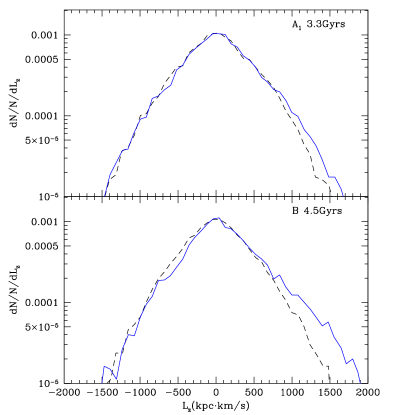
Figure 13: Distribution of z-component of the angular momentum of dark matter particles at different moments. Dashed and full curves are for initial and advanced moments (3.3 Gyrs for A₁ and 4.5 Gyrs for B) of evolution. We present results only for 10000 particles, which initially were in a spherical shell centered at 3 kpc. Particles at other radii showed even smaller effects. The changes in the angular momentum are clearly seen in both models: there are more particles with high angular momentum. This indicates that the dynamical friction transfers some angular momentum to the dark matter, but the effect is extremely weak.

To summarize, we clearly find indications of the dynamical friction between the dark matter and the stellar component. Nevertheless, the amount of the angular momentum lost by the stellar particles is very small: about 5% during 5 Gyrs of evolution. There is much larger exchange of the angular momentum between stellar particles. Most of this exchange happens during the formation of the bar. Once the bar is in place, the distribution of the angular momentum changes very little.

6 Structure of bars: the pattern speed and the surface density

Figure 10 shows the evolution of the pattern speed and the amplitude of the bars in our simulations. Models A₁ and B evolve qualitatively similar. After different periods of time models A₁ and Bform a bar which rotates with almost constant speed for about 5 Gyrs. The amplitude of the bar in the model B experienced a noticeable decline (a factor of two) at 2 Gyrs. This change in the amplitude was not accompanied by any other obvious changes. For example, the pattern speed did not change.

The bar pattern speed is slightly larger in model B ($\approx 33\,\rm{km}\,\rm{s}^{-1}/\,\rm{kpc}$) as compared with model A₁ ($\approx 27\,\rm{km}\,\rm{s}^{-1}/\,\rm{kpc}$). What is remarkable about the pattern speeds is that they do not change much. For example, in model A₁ the bar changed its frequency from $\approx 27\,\rm{km}\,\rm{s}^{-1}/\,\rm{kpc}$ when it formed to $\approx 20\,\rm{km}\,\rm{s}^{-1}/\,\rm{kpc}$ at $t=8.5$ Gyrs.

The evolution of model A₂ is very different. For the first 3 Gyrs the bar was very quickly rotating with the pattern speed of $\approx 50\,\rm{km}\,\rm{s}^{-1}/kpc$ - almost twice larger than in model A₁. At later moments the pattern speed was declining. It went down to $\approx 25\,\rm{km}\,\rm{s}^{-1}/kpc$ by the end of evolution.

In order to find how fast is the bar rotation, we show in the Figure 14 the bar pattern speeds, the rotation, and the circular velocity curves for the models. The thick horizontal bars in the plots indicate the length of the bars. The corotation radius can be identified as the radius of intersection of the bar pattern speed with the rotation curve. In all three models the bars rotate fast with the ratio of the corotation radius to the bar length equal to ${\cal R}\approx 1.2-1.7$.

Figure 14: Different frequencies in models A₁, A₂, and B. The full curves show the frequency of rotation of the disk $\Omega_{\rm rot}\equiv V_{\phi}/R$. The dashed curves present the frequency of rotation for a cold disk $\Omega_{\rm circ}\equiv\sqrt{GM/R^{3}}$. The difference between the two frequencies are due to the asymmetric drift. The dotted horizontal lines show the frequency of rotation of the bars. The extension of the bars in the models is indicated by the thick lines. The distance of a bar from the rotation curves is a measure of how fast is the bar. The bar in the model B is clearly a very fast bar, which extends almost up to the corotation. The bars in models $A$ rotate slower, but they are still fast bars.

Figure 15 shows the surface density profiles of the stellar components in the models. The surface density profiles seems to indicate a development of normal galactic components: an exponential disk and a (exponential) bulge. Note that even after significant evolution in the central part, the outer part of the disk (radii larger than 5 kpc) is still well approximated by a simple exponential profile. Still, there is a change even in the outer part: the exponential scale-length increases quite substantially - by a factor of 1.5.

Figure 15: Surface density profiles of the stellar components for models A₁, A₂, and B. The full curves present the azimuthally averaged profiles. Dashed curves show double exponential fits with parameters presented in the plots. The dotted curves show the surface density along the major axes of the bars. The surface densities along the minor bar axis are shown with the dot-dashed curves. All the curves are obtained by averaging over three time moments covering about 0.5 Gyr. For comparison a large dot shows the surface density of the disk (stars + gas) for our Galaxy at the solar position.

7 Discussion

Bars in our models are different from what was found in simulations of Debattista & Sellwood (2000). In two of our dark matter-dominated models bars do not show a strong tendency to slow down. This contradicts results of Debattista & Sellwood (2000), who always find that the pattern speed of bars substantially declines with time. We tried to find an explanation for the disagreement. Numerical effects are the obvious first suspects. The force resolution in the Debattista & Sellwood (2000) models was more than an order of magnitude lower than in our simulation. In an effort to reproduce at least some conclusions of Debattista & Sellwood (2000), we re-run model A₁ with the resolution comparable with that in models of Debattista & Sellwood (2000). The evolution was so much affected by the lack of the resolution that after running the model for more than 2 Gyrs and not finding even a hint of a bar, we abandoned the simulation. We then re-started the simulation with decreased “thermal” velocities in the disk. The $Q$ parameter was set at the value $Q=0.05$ used by Debattista & Sellwood (2000). In this simulation a bar forms. Figure 16 shows that the pattern speed decreases very substantially over a relatively short period of time - more or less in line with what was found by Debattista & Sellwood (2000). Thus, we find the same behavior of bars – declining pattern speed – if we substantially reduce the resolution and reduce the random velocities of disk particles. The angular momentum of the stellar particles also was declining faster than in the high resolution run. This exercise clearly demonstrates that the force resolution and the stellar velocities are important factors. In our simulations the low force resolution produced erroneous results that the bar pattern speed declines with time. The “coldness” of the disk may also have affected the pattern speed. This has also been reported by Athanassoula (2003).

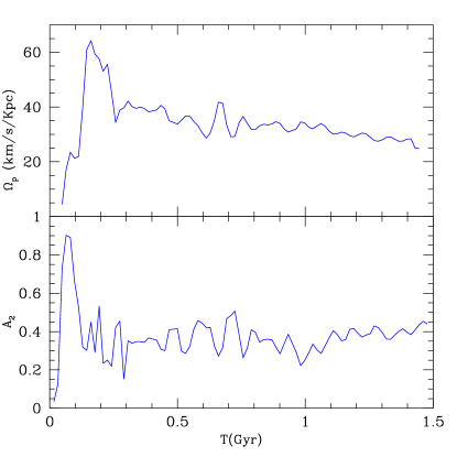
Figure 16: Evolution of the pattern speed and the bar amplitude in a simulation with initially cold disk with $Q=0.05$. Other parameters of the simulation are the same as for model A₁. The simulation was done with a very low resolution of 0.5 kpc to mimic results of Debatista & Sellwood (2000). In this case the pattern speed quickly decreases with time giving an impression that the bar is slowed down by the dynamical friction with the dark matter. This “slowing down” of the bar is an artifact of unrealistically cold disk and grossly insufficient force resolution.

Length is another important property of bars. In our simulations bars have radii comparable to both initial and final exponential disk length. This is quite different from what, for example, Athanassoula & Misiriotis (2002) find. The bar length in their models is more than three times longer than the initial disk scale-length. After 8.5 Gyrs of evolution ($t\approx 610$ in units used by Athanassoula & Misiriotis (2002)) the bar length in our A₁ model is $6-6.5\,\rm{kpc}$ as compared with $10-14\,\rm{kpc}$ for model MH in Athanassoula & Misiriotis (2002). Bars are also very long in the models of Debattista & Sellwood (2000): they span the entire disk. Even that a comparison with disk scale-length after bar formation could be more favored for those models it is interesting to test how numerical resolution may affect the bar length. We rerun model A₂ with a formal resolution of 350 pc which is 1.6 times the formal resolution of Athanassoula & Misiriotis (2002). Figure 17 shows the distribution of stellar particles of the simulations for model A₂ at different moments of time. The system was clearly affected by the resolution. At 2 Gyrs the bar is barely visible in the high resolution run, but it is much longer and stronger in the low resolution run. The differences are not as large at later moments, but even at later moments the differences are substantial. This example shows that the bar length is quite sensitive to the effects of the resolution. Short bars are also formed in high resolution simulations of Sellwood (2002).

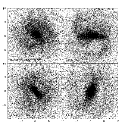
Figure 17: Effects of resolution on bar formation in model A₂. Left panels show stellar particles in the simulation, which reached 20 pc resolution. Right panels show the same model simulated with the resolution limited to 350 pc. The top panels are for 2 Gyrs after initial moment; the bottom panels are for 4.5 Gyrs. The high resolution run has a very short (1 kpc) bar for 3 Gyrs, while the low resolution run has remarkably strong and long bar from the very beginning. Axes are labeled in units of kpc. This figure illustrates that numerical resolution can significantly affect structure of a bar. Lack of resolution results in longer and stronger bars.

We may only speculate why a better force resolution leads to shorter and weaker bars. Orbital resonances are traditionally blamed for the growth of bars. Fast rotating bars trap particles. This in turn increases the strength of the bar. It gets longer and more massive trapping even more trajectories. Low force and high mass resolutions make the system more resonant by producing a gravitational potential with too shallow gradients. Motion of particles in such potentials can be more susceptible to resonances. Thus, we get longer bars. Increased force resolution results in steeper gradients of the density and the potential. As the result, particle trajectories do not stay as much in resonances, which decreases the rate of the growth of the bar. A central concentration makes bars weaker and can even destroy them (e.g., Norman et al., 1996). During first stages of bar formation the central concentration increases very dramatically (see Figures 8 and 9). A low force resolution artificially makes the central concentration shallower. This may result in longer and stronger bars, which are known to rotate slower. The comparison of the low and high resolution runs of the model A₂ supports this picture.

Numerical effects are clearly important for the structure of the system. Still, they can not explain all the differences between our results and those of Athanassoula & Misiriotis (2002). The bar in the low resolution run of A₂ model is longer than in the high resolution run. Still, it is shorter than what was found by Athanassoula & Misiriotis (2002). The remaining differences are likely due to the differences in the overall structure of the system. Our halo was significantly more extended (250 kpc as compared with 50 kpc in Athanassoula & Misiriotis (2002)). Thus, the dark matter particles have larger velocities. Our disk is also slightly “hotter”. Each effect points in the same direction: systems studied by Athanassoula & Misiriotis (2002) are likely more susceptible to resonances. The effects accumulate over billions of years producing longer bars in Athanassoula & Misiriotis (2002). Athanassoula (2003) presents a similar and more extensive discussion which conclude that a hotter system is less resonant and has a slower decline of the bar pattern speed and a lower rate of bar growth. In particular Athanassoula (2003) shows that bars in disks with a Toomre parameter $Q=.1$ slow down more thant four times faster than in a disk with $Q=2.2$, this result is in agreement with our discussion. We can conclude that the structure and kinematics of halo and disk have a central role in bar evolution. Differences within our simulations and previous works like Athanassoula & Misiriotis (2002)) are influenced not only by resolution but also by the different structure of the models.

It is still a matter of debate which initial setup is more realistic. Our halos are consistent with predictions of cosmological models. They extend to the virial radius; they have realistic profiles and rotation curves. Halos in Athanassoula & Misiriotis (2002) produce reasonable rotation curves although they are not consistent with cosmological models. In any case, we do not confirm Athanassoula & Misiriotis (2002) conclusions that bars in models with centrally concentrated dark matter are necessarily too long (3-4 disk initial exponential lengths). Their results are valid only for the particular models they studied. They are not valid as a general statement that realistic dark matter models should have excessively long bars. While we have mentioned some disagreements with Athanassoula & Misiriotis (2002), it should be emphasized, that we find many similar results at least on the qualitative level. In agreement with Debattista & Sellwood (2000) and Athanassoula & Misiriotis (2002) we find that a massive dark matter halo does not prevent formation of a strong bar. We also find that bars have a tendency to grow with time and do not dissolve spontaneously. We agree with Athanassoula & Misiriotis (2002) that formation of a bar leads to a baryon-dominated central region even in cases when the disk is initially submaximal. We also find that formation and evolution of bars does not lead to a decline in the density of the dark matter in the central region.

It is an interesting question how a bar can possibly not slow down when it rotates inside a dense dark matter halo. Even in model A₁ the disk lost 6 percent of its angular momentum after 5 Gyrs of evolution. One should expect that most of the loss comes from the bar. Because the bar has only 40% of the stellar mass, one expects that the bar should lose around 15% of its angular momentum. This is still marginally consistent with the behavior of the pattern speed in Figure 10. Still, what if $\Omega_{p}$ is really constant? Can a bar rotate with the constant speed and lose its angular momentum? If we believe the arguments presented by Weinberg (1985), the answer is “No”. Indeed, if a solid rotating bar, often used in these kind of estimates (Weinberg, 1985; Little & Carlberg, 1991; Weinberg & Katz, 2001), loses its angular momentum, it must slow down. Yet, real bars may behave differently because they are not solid objects. Bars are made of particles, which stream through them creating a wave pattern, which we call a “bar”. When the bar loses angular momentum, it is individual particles which lose it. The particles can move to orbits with smaller radii where orbital frequency is larger. It is reasonable to assume that the bar speed is proportional to the orbital frequency of particles. Because the particles rotate with larger frequency, the bar can speed up when it loses the angular momentum. Real bars have another feature, which complicates things even more. Typically, they have a tendency to grow. For example, the bar in model A₁ has increased its length from $\approx 4-5\,\rm{kpc}$ at 3 Gyrs to $\approx 6-6.5\,\rm{kpc}$ at 5 Gyrs. This 30% increase in the bar length is due to particles, that came from large radii. Because the rotation curve is nearly flat, particles at larger radii have smaller orbital frequencies. When they “join” the bar, it will have a tendency to slow down. This happens if the particles do not significantly change trajectories. If the particles lose their angular momentum and decrease average radius, they may cause the bar to speed up.

The outcome of all these competing processes is difficult to predict. We find that slow growing bars rotate with almost constant speed (e.g., bars in models A₁, B, and the bar in model A₂ at $t<3$ Gyrs). If a bar grows fast, it significantly decreases its pattern speed. This happened in model A₂ at $t=3-5$ Gyrs. At 3 Gyr the bar was very short ($\sim 1.5\,\rm{kpc}$) and weak. At earlier moments of time it was growing very slowly and was rotating with high constant speed for almost 3 Gyrs. At $t\approx 3$ Gyrs the bar starts to grow very fast. By the end of evolution (6 Gyrs) it was 4.5 – 5  kpc long and it slowed down by a factor of two.

Do bars in our models rotate as fast as the observed bars? In our models bars have ${\cal R}=1.2-1.7$. This should be compared with the observational results. Unfortunately the number of galaxies, for which the direct method of Tremaine & Weinberg (1984) was used, is small and the errors are still large. For NGC 936 (Sa type) Merrifield & Kuijken (1995) find ${\cal R}=1.4\pm 0.3$. Gerssen et al. (1999) find ${\cal R}=1.15^{+0.38}_{-0.23}$ for S0 galaxy NGC 4596. For five S0 galaxies Aguerri et al. (2003) find that “${\cal R}$  is consistent with being in the range from 1.0 to 1.4”. Taken at the face value, these results are not consistent with most of our bars, which typically have ${\cal R}\approx 1.5$. Yet, on pure statistical grounds our bars are still acceptable because the errors of the quoted observational results are only $1\sigma$’s. For example, at the $2\sigma$ level, the five galaxies studied by Aguerri et al. (2003, Table8) give the following upper limits: ${\cal R}<1.4$ (ESO 139-G009), $<2.8$ (IC 874), $<1.6$ (NGC 1308), $<1.9$ (NGC 1440), and $<2.3$ (NGC 3412). Our bars are well within the limits.

There is another alarming issue: the overall structure of early type – S0 and Sa – spirals studied in the observations is very different from that of the numerical models. The later aim at Sb and Sc types, not S0. The surface density in simulations is well described by the double exponential law (Figure 15) ; the stellar velocity dispersion is relatively small (Figures 2-3). The situation is very different for the galaxies studied by Aguerri et al. (2003). Surface brightness profiles are not even close to double exponentials. Every galaxy requires four components: a central bulge, a bar, a lens, and a disk (Figure 7, Aguerri et al., 2003). For example, NGC 3412, which has circular velocity $205\,\rm{km}\,\rm{s}^{-1}$ (close to our models), is dominated in the central $\sim 1\,\rm{kpc}$ region by a bulge, which does not have any counterpart in the simulations. A massive lens component is important at around $3\,\rm{kpc}$. Again it does not exist in our models. Line-of-sight velocities are also significantly larger than what we have in the models. While it is clear that we are dealing with very different objects, one may only speculate how these differences affect ${\cal R}$. Combes & Elmegreen (1993) find that early type spirals should have faster rotating bars. If that is confirmed for models with live bulges and halos, disagreements with observations may become smaller. In the same direction point results of Athanassoula (2003), who finds that bars in hotter disks rotate faster.

In order to resolve the issues, numerical models should be improved to mimic S0 galaxies. Models likely should include a small initial bulge and should have disks with larger random velocities. Observations should also be done for Sb and Sc galaxies. Before this is done, it is difficult to assess the situation. As it stands now, differences with observations are not large and models cannot be rejected.

8 Conclusions

We study formation of bars in galactic models with equilibrium exponential disks rotating inside extended dark matter halos predicted by modern cosmological models. The amount of the dark matter in the central 10 kpc region is substantial - it is larger than the disk mass. Our models have parameters, which approximately match those of the Milky Way galaxy: the virial mass is $(1-2)\times 10^{12}{\rm M}_{{}_{\mathord{\odot}}\;}$, the total mass of the disk and the bulge is $(4-6)\times 10^{12}{\rm M}_{{}_{\mathord{\odot}}\;}$. Dark matter halos in our models extend to the virial radius of 200-300  kpcand have cuspy inner profiles. We use millions of particles to simulate the models.

Extended strong bars form in all our models in spite of the fact that the random velocities are much larger than the kinetic energy of disk rotation. Our results are at odds with the Ostriker-Peebles criterion of bar stability. We find that the dynamical friction between the dark matter and the bar results in some transfer of angular momentum to the dark matter halo, but the effect is much smaller then previously found in low resolution simulations and is incompatible with early analytical estimates. The mass and the force resolutions are crucial for the dynamics of bars. In simulations with the low resolution of 300-500 pc we find that the bar slows down and the angular momentum is lost relatively fast. In simulations with millions of particles, which reach the resolution of 20-40 pc, the pattern speed may not change over billions of years and the stellar component loses very little (5 – 10%) of its total angular momentum.

Bars in our models are fast rotators with the ratio of the corotation radius to the bar major semi-axis being in the range ${\cal R}=1.2-1.7$, which is marginally compatible with observational results. The initial random velocities of the disk in the central $\approx 1-2\,\rm{kpc}$ region can substantially affect the structure of bars. In our simulations “hot” disks develop a longer bar, which rotates at an almost constant pattern speed. Colder models generate an initially shorter bar, which grows and slows down.

In contrast to many previous simulations, bars in our models are relatively short. As in many observed cases, the major bar semi-axis in the models is about an exponential length of the disk.

The transfer of the angular momentum between inner and outer parts of the disk plays a very important role in the secular evolution of disk. The main effect is the angular momentum transfer from the central part of the bar to the outer disk. This transfer leads to a substantial increase of the stellar mass and to a decrease of the dark matter-to-baryons ratio in the centre of the galaxy. For the Milky Way- scale models the central 2 kpc is strongly dominated by the baryonic component after 1 – 2 Gyrs since the onset of the instability. At intermediate 3 –10 kpc scales the disk is sub-dominant: spherically average density of the disk is 2-3 times smaller than the density of the dark matter. This makes an interesting twist for the never ending debate between supporters and opponents of the maximum disks. We predict that barred galaxies (or galaxies, which were barred) in the central region ( $\sim$ 1/2 of the disk exponential length) should have the maximum disk (maximum bulge or bar, to be more precise), but the outer part is the sub-maximum disk.

Another effect of the bar formation is the increase by a factor of $\approx 1.2-1.5$ of the exponential length of the disk. This increase may change theoretical predictions for the disk lengths in hierarchical models.

We find that the surface density profile of an evolved system is well approximated by a double exponential law. The 1/4 law for the bulge gives a worse fit, but it is not excluded. Only in extreme cases (very late stages of evolution, very strong bars formed in low resolution simulations) we see a tendency for a bar to produce a flat part of the surface density in the interface of the bar and the disk.

To summarize, we use more realistic models than in most of previous simulations and find that the models with substantial amount of the dark matter produce bar structure in striking agreement with observational results.

References

- Aguerri et al. (2003) Aguerri J. A. l., Debattista V. P., Corsoni E. M., 2003, MNRAS, 338, 465
- Athanassoula (2003) Athanassoula E., 2003, astro-ph/0302519 to appear in MNRAS, 000, 000
- Athanassoula & Misiriotis (2002) Athanassoula E., Misiriotis A., 2002, MNRAS, 330, 35
- Berentzen et al. (1998) Berentzen I., Heller C. H., Shlosman I., Fricke K. J., 1998, MNRAS, 300, 49
- Binney & Tremaine (1987) Binney J., Tremaine S., 1987, Galactic dynamics. Princeton, NJ, Princeton University Press, 1987, 747 p.
- Binney & Evans (2001) Binney J. J., Evans N. W., 2001, MNRAS, 327, L27
- Blitz & Spergel (1991) Blitz L., Spergel D. N., 1991, ApJ, 370, 205
- Colín et al. (2000) Colín P., Klypin A. A., Kravtsov A. V., 2000, ApJ, 539, 561
- Combes & Elmegreen (1993) Combes F., Elmegreen B. G., 1993, AAP, 271, 391
- Combes & Sanders (1981) Combes F., Sanders R. H., 1981, A&A, 96, 164
- Contopoulos (1981) Contopoulos G., 1981, AAP, 104, 116
- de Blok et al. (2001) de Blok W. J. G., McGaugh S. S., Rubin V. C., 2001, AJ, 122, 2396
- Debattista & Sellwood (1998) Debattista V. P., Sellwood J. A., 1998, ApJ, 493, L5
- Debattista & Sellwood (2000) Debattista V. P., Sellwood J. A., 2000, ApJ, 543, 704
- Dehnen & Binney (1998) Dehnen W., Binney J., 1998, MNRAS, 294, 429
- Eke et al. (2001) Eke V. R., Navarro J. F., Steinmetz M., 2001, ApJ, 554, 114
- El-Zant et al. (2001) El-Zant A., Shlosman I., Hoffman Y., 2001, ApJ, 560, 636
- Elmegreen & Elmegreen (1985) Elmegreen B. G., Elmegreen D. M., 1985, ApJ, 288, 438
- Flores & Primack (1994) Flores R. A., Primack J. R., 1994, ApJ, 427, L1
- Freudenreich (1998) Freudenreich H. T., 1998, ApJ, 492, 495
- Fridman & Poliachenko (1984) Fridman A. M., Poliachenko V. L., 1984, Physics of gravitating systems - Vol.1: Equilibrium and stability; Vol.2: Nonlinear collective processes: Nonlinear waves, solitons, collisionless shocks, turbulence. Astrophysical applications. New York: Springer, 1984
- Fux (1997) Fux R., 1997, Astronomy & Astrophysics, 327, 983
- Gerhard (2002) Gerhard O., 2002, astro-ph/0203109
- Gerssen et al. (1999) Gerssen J., Kuijken K., Merrifield M. R., 1999, MNRAS, 306, 926
- Hammersley et al. (1999) Hammersley P. L., Cohen M., Garzón F., Mahoney T., López-Corredoira M., 1999, MNRAS, 308, 333
- Hernández et al. (2001) Hernández X., Avila-Reese V., Firmani C., 2001, MNRAS, 327, 329
- Hernquist (1993) Hernquist L., 1993, ApJS, 86, 389
- Hernquist & Weinberg (1992) Hernquist L., Weinberg M. D., 1992, ApJ, 400, 80
- Hohl (1971) Hohl F., 1971, ApJ, 168, 343
- Klypin et al. (1999) Klypin A., Kravtsov A. V., Valenzuela O., Prada F., 1999, ApJ, 522, 82
- Klypin et al. (2002) Klypin A., Zhao H., Somerville R., 2002, ApJ, 573, xx
- Knebe et al. (2000) Knebe A., Kravtsov A. V., Gottlöber S., Klypin A. A., 2000, MNRAS, 317, 630
- Kravtsov (1999) Kravtsov A. V., 1999, PhD
- Kravtsov et al. (1998) Kravtsov A. V., Klypin A. A., Bullock J. S., Primack J. R., 1998, ApJ, 502, 48
- Kravtsov et al. (1997) Kravtsov A. V., Klypin A. A., Khokhlov A. M., 1997, ApJS, 111, 73
- Little & Carlberg (1991) Little B., Carlberg R. G., 1991, MNRAS, 251, 227
- Łokas (2001) Łokas E. L., 2001, MNRAS, 327, L21
- Merrifield & Kuijken (1995) Merrifield M. R., Kuijken K., 1995, MNRAS, 274, 933
- Merritt & Sellwood (1994) Merritt D., Sellwood J. A., 1994, ApJ, 425, 551
- Miller (1978) Miller R. H., 1978, ApJ, 224, 32
- Moore (1994) Moore B., 1994, Nature, 370, 629
- Moore et al. (1999) Moore B., Ghigna S., Governato F., Lake G., Quinn T., Stadel J., Tozzi P., 1999, ApJ, 524, L19
- Navarro et al. (1997) Navarro J. F., Frenk C. S., White S. D. M., 1997, ApJ, 490, 493
- Navarro & Steinmetz (2000) Navarro J. F., Steinmetz M., 2000, ApJ, 528, 607
- Nelson & Tremaine (1999) Nelson R. W., Tremaine S., 1999, MNRAS, 306, 1
- Norman et al. (1996) Norman C. A., Sellwood J. A., Hasan H., 1996, ApJ, 462, 114
- Ostriker & Peebles (1973) Ostriker J. P., Peebles P. J. E., 1973, ApJ, 186, 467
- Raha et al. (1991) Raha N., Sellwood J. A., James R. A., Kahn F. D., 1991, Nature, 352, 411
- Sellwood (2002) Sellwood J. A., 2002, private communication
- Sellwood & Athanassoula (1986) Sellwood J. A., Athanassoula E., 1986, MNRAS, 221, 195
- Shen & Sellwood (2003) Shen J., Sellwood J. A., 2003, astro-ph/, 0303130
- Toomre (1981) Toomre A., 1981, in Structure and Evolution of Normal Galaxies What amplifies the spirals. pp 111–136
- Tremaine & Weinberg (1984) Tremaine S., Weinberg M. D., 1984, ApJ, 282, L5
- van den Bosch & Swaters (2001) van den Bosch F. C., Swaters R. A., 2001, MNRAS, 325, 1017
- Weinberg (1985) Weinberg M. D., 1985, MNRAS, 213, 451
- Weinberg (1998) Weinberg M. D., 1998, MNRAS, 297, 101
- Weinberg & Katz (2001) Weinberg M. D., Katz N., 2001, astro-ph, 1, 0110632
- Zhao & Mao (1996) Zhao H., Mao S., 1996, MNRAS, 283, 1197
- Zhao (1996) Zhao H. S., 1996, MNRAS, 283, 149