Tracing the Mass during Low-Mass Star Formation. III. Models of the Submillimeter Dust Continuum Emission from Class 0 Protostars
Abstract
Seven Class 0 sources mapped with SCUBA at 850 and 450 µm are modeled using a one dimensional radiative transfer code. The modeling takes into account heating from an internal protostar, heating from the ISRF, realistic beam effects, and chopping to model the normalized intensity profile and spectral energy distribution. Power law density models, , fit all of the sources; best fit values are mostly , but two sources with aspherical emission contours have lower values (). Including all sources, . Based on studies of the sensitivity of the best-fit to variations in other input parameters, uncertainties in for an envelope model are . If an unresolved source (e.g., a disk) contributes of the flux at the peak, is lowered in this extreme case and . The models allow a determination of the internal luminosity ( L⊙) of the central protostar as well as a characteristic dust temperature for mass determination ( K). We find that heating from the ISRF strongly affects the shape of the dust temperature profile and the normalized intensity profile, but does not contribute strongly to the overall bolometric luminosity of Class 0 sources. There is little evidence for variation in the dust opacity as a function of distance from the central source. The data are well-fitted by dust opacities for coagulated dust grains with ice mantles (Ossenkopf & Henning 1994). The density profile from an inside-out collapse model (Shu 1977) does not fit the data well, unless the infall radius is set so small as to make the density nearly a power-law.
1 Introduction
Modern theories of star formation predict the evolution of the density structure, , and velocity structure, , of the gas and dust envelope of protostars. Optically thin dust emission at submillimeter wavelengths provides an observational constraint on the density distribution of the protostellar envelope and therefore constrains theoretical models of star formation.
Class 0 protostars represent an early, highly embedded phase during the formation of low mass stars ( few M⊙). The original evolutionary sequence for low mass protostars (Class I, II, and III) is based on the shape of the spectral energy distribution (SED) from observations at near and mid-infrared wavelengths (Lada 1987). Low mass protostars are thought to evolve from a thick dusty envelope where most of the energy is re-radiated by dust in the far-infrared (Class I) to progressively less embedded objects with near and mid-infrared excesses from dusty disks (Class II or classical T Tauri stars and Class III or weak-line T Tauri stars). The discovery of extremely embedded objects with submillimeter telescopes led to a new class of protostars, Class 0 objects, which are so highly enshrouded that their near infrared emission has generally not been detected and their SEDs peak longward of 100 µm. Observationally, Class 0 sources are cores that have , where is the total luminosity detected longward of 350 µm (André et al. 1993). Alternatively, Class 0 sources are characterized by K, where is the temperature of a blackbody with the same mean frequency as the observed SED (Chen et al. 1995). Based on the relative numbers of Class 0 and Class I objects, it has been argued that the timescale for Class 0 objects is short, perhaps years (André et al. 2000). Class 0 objects have powerful outflows, which suggest high accretion rates (Bontemps et al. 1996). As data improve, some Class I sources are being reclassified to Class 0 sources (e.g., Shirley et al. 2000, Young et al. 2001), suggesting a reexamination of this argument (see also Visser, Richer, & Chandler 2001).
It is important to understand the structure of the envelope of Class 0 objects since they are likely to be the earliest observed phase of star formation with a central accreting protostar (André et al. 2000). The emission from an optically thin dust shell observed at an impact parameter, , with dust opacity, , that does not vary with radius, is given by
| (1) |
(Adams 1991), where is the outer radius. For an optically thin envelope (at all wavelengths) dominated by a central source of luminosity, , the dust temperature distribution can be approximated by a power law:
| (2) |
where (cf. Doty & Leung 1994) and is the power law exponent of the dust opacity (), which typically lies between 1 and 2 in the submillimeter. If we also assume the density distribution follows a power law, , then in the Rayleigh-Jeans limit (), the specific intensity integral simplifies to , where . Previous studies of the density structure of Class 0 objects assumed a temperature power law of the form (Walker et al. 1990, Ladd et al. 1991, Chandler & Richer 2000, Hogerheijde & Sandell 2000, Shirley et al. 2000, and Motte & André 2001). However, this approach is valid in the outer envelopes of low luminosity sources due to a breakdown in the Rayleigh-Jeans approximation at wavelengths shorter than 1 mm and due to external heating from the interstellar radiation field (ISRF) (Shirley et al. 2000). It then becomes necessary to calculate self consistently in the integral in Equation (1) to reveal the density distribution of the envelope.
In Paper I (Shirley et al. 2000), 21 low mass cores within 325 pc were observed at 850 µm and 450 µm using the Submillimeter Common User Bolometer Array (SCUBA) (Holland et al. 1999) on the JCMT 15-m radio telescope. Thirteen sources from the original sample were classified as Class 0, three sources having been previously classified as Class I. In this paper, we present 1D dust radiative transfer models for seven of the Class 0 sources selected for spatial isolation and high signal-to-noise radial profiles (): B335, B228, L723, IRAS03282+3035, L1448C, L1527, and L483. B335, B228, IRAS03282+3035, and L1448C appear circular in the dust continuum maps down to the 20% contour, while L1527, L483, and L723 are clearly aspherical at that level. The bolometric temperature ranges from 23K (IRAS03282+3035) to 52K (L483) and the bolometric luminosity ranges from 1.2 L⊙ (IRAS03282+3035 and B228) to 13 L⊙ (L483). In Paper II (Evans et al. 2001), three pre-protostellar cores (L1512, L1544, and L1689B) were modeled using one-dimensional radiative transfer and a beam convolution code. In this paper, the seven Class 0 sources will be modeled using the same procedure used in Paper II, with the addition of an internal luminosity source. The modeling procedure and inputs are discussed in Section 2. We use B335 as a test object (Section 3.1) to model the sensitivity to the model input parameters. Individual sources are modeled in Sections 3 and 4, while the implications of our best fit models are discussed in Section 5.
2 1D Dust Radiative Transfer Modeling
The 1D dust models are calculated from a modified version of the Egan, Leung, and Spagna (1984) continuum radiative transfer code. This code iteratively calculates the equilibrium dust temperature on a 1D radial grid by simultaneously solving the combined moment radiative transport equations in quasi-diffusion form and the energy balance equations as a two-point boundary value problem. The radiation field is constructed by solving a set of ray equations along impact parameters, , through the cloud. There are four physical inputs to the radiative transfer code: the density distribution, ; the internal source luminosity, ; the scaling factor for the interstellar radiation field, ; and the dust opacity, . In addition, the radial grid (100 points) and impact parameters, as well as the wavelength grid (59 wavelengths) are chosen to cover the relevant range so that results are insensitive to the details of these grids. The equilibrium dust temperature distribution, , which is the output from the dust code, is used by an observation simulation code (Paper II) to calculate the normalized radial intensity profiles, , by solving Equation (1), performing beam convolutions, and simulating chopping. The code also models the observed SED, , by convolving the model intensity with the beam () used in each observation.
The internal radiation field is assumed to be a blackbody with an effective temperature of 6000 K. Since all of the objects we are modeling are very opaque at near-infrared wavelengths, the exact shape of the spectrum of the internal radiation field is not important; only the total internal luminosity is important. The shape of the ISRF was determined from COBE results (Black 1994) plus the cosmic microwave background (CMB) and the ultraviolet component of the ISRF () from van Dishoeck (1988). This ISRF is considerably stronger in the infrared than the previous versions of the ISRF (Mathis, Mezger, & Panagia 1983) (see Figure 2 of Paper II for a plot of the different ISRFs). We modify the strength of the ISRF by multiplying all portions of the ISRF spectrum except the CMB with a factor denoted by . For the models discussed in this paper, we used a coarse grid with , , and . These factors for the far-UV (FUV) portion of the ISRF correspond to 0.45, 1.5, and 4.5 respectively, where is integrated FUV flux between nm and nm in units of erg s-1 cm-2 (cf. Hollenbach et al. 1991). In Paper II, the best fit to the observed radial profiles and SED suggest a lower strength to the ISRF ().
The dust opacity, , was taken from the models of Ossenkopf and Henning (1994) for grains that have coagulated for yr at a density of cm-3, both with (OH5) and without (OH2) accreted ice mantles. We assume a gas to dust ratio of 100 by mass to convert OH5 opacities (per gram of dust) to opacity per gram of gas. OH5 opacities have been successful at reproducing the SED of both high mass (van der Tak et al. 2000) and low mass star forming cores (Paper II). OH5 opacities at submillimeter wavelengths can be approximated by a power law () with and an opacity of cm2 per gram of gas at 850 µm. The OH2 dust opacities are lower at far-infrared wavelengths but up to 1.6 times higher at submillimeter and millimeter wavelengths than OH5 dust opacities. The cross-over point is near 350 µm (see Fig. 2 of Paper II).
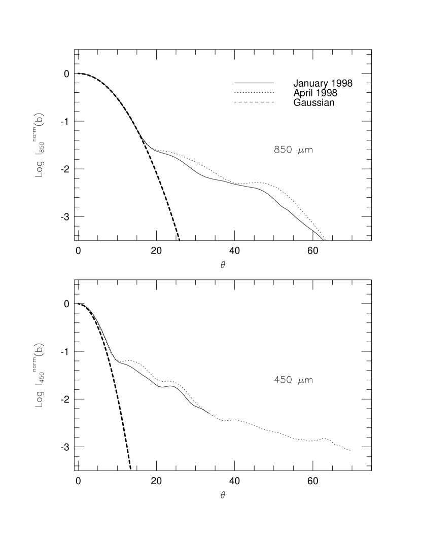
The JCMT beams derived from AFGL618 and Uranus were used for the beam convolution of the model profiles at 850 and 450 µm (see Figure 1). It is very important to convolve the model specific intensity distribution with a realistic beam profile to derive an accurate estimate of the envelope density distribution. Using a gaussian beam shape instead of the actual beam profile can profoundly distort the interpretation of the power law index, , by up to 0.5 (Shirley et al. 2000). Since the beam shape was stable during the second half of the night in April 1998 (see Paper I), nine Uranus profiles were added together to use an average beam profile with high signal-to-noise out to 70″ from the center of the map. No planets were available to make beam maps for the January 1998 sources (L1527, IRAS03282, L1448C); so the secondary calibrator, AFGL618 was observed. The January 1998 observations were taken in the first half of the night when the beam shape is not so stable and changes shape continuously as the telescope cools. AFGL618 is much weaker than Uranus at 850 and 450 µm; therefore the beam maps have much lower signal-to-noise at large radii. The January beam map was produced by averaging together three AFGL618 maps observed during the same time of night that our objects were observed. Because the 450 µm profile of AFGL618 becomes too noisy beyond 34″, the average Uranus beam profile from April was used for the 450 µm January beam beyond 34″. These beam calibration difficulties introduce larger uncertainties, , in the best fit models for the January sources.
Many of the radial profiles from Paper I show a turn-down in the intensity profile beyond 60″ from the center of the map. This turn-down could be due to a steepening of the density profile or due to the effects of chopping. To test the possibility of a steeper density profile, we must account for the chop throw. The SCUBA observations were chopped in azimuth with a 120″ chop throw. Since the SCUBA array is 2D, all of the positions within a single annulus chop different distances from the center of the map. Therefore, our 1D model can only include an approximate simulation of the true effects of chopping. The details of how we simulate chopping has a noticeable effect on the shape of the model intensity profiles beyond 60″; consequently, we do not attempt to model normalized intensity profiles beyond this radius.
The agreement between the model and the data can be quantified in terms of the reduced chi-squared for the normalized intensity profile at wavelength :
| (3) |
where is the azimuthally averaged, normalized intensity in a circular aperture at impact parameter , is the uncertainty in the data, and is the number of impact parameters. Only points spaced by a full beam are used in computing to avoid introducing correlations. We calculate for the 850 and 450 µm profiles and define as the sum of and . The signal-to-noise was higher for the 850 µm maps and therefore the has the most weight in determining the best fit.
The agreement between the model SED and the observed one is quantified by , calculated from a similar equation:
| (4) |
where is the observed flux into a beam and is the modeled flux into the same beam. When photometry at the same wavelength with different beams exists, the points are both considered in calculating . Wavelengths shorter than 60 µm are not included because they are expected to be optically thick and therefore very sensitive to asymmetric geometries (e.g., outflow cavities, flattened envelopes), which we are currently unable to model. In addition, much of the far-infrared photometry has large and uncertain calibration errorbars, and the opacities as a function of frequency are uncertain. For all these reasons, poor fits to the SED are not considered a serious problem in constraining the density distribution; however we often find that the best , which considers only the profiles, occurs for the model with the best .
In fact, the SED and the normalized radial intensity profiles provide nearly orthogonal constraints on model parameters (§3). The SED is sensitive to the strength of the ISRF and a massopacity product (Paper II). In particular, the flux density at 850 µm constrains the mass, while the full SED provides information on the the variation of dust opacity with frequency, subject to the caveats mentioned above. Measurements of the flux density into different beams at the same wavelength provides some constraint on the density distribution, but the shape of the density distribution is much better constrained by the normalized radial profile ().
The simplest models to test are single power laws,
| (5) |
in cm-3 for the gas density. The density, , is normalized to a fiducial radius, , of 1000 AU and represents the total gas number density (, ). There are seven parameters in the power law models: the power law exponent, ; the density at a fiducial radius, ; the inner radius, ; the outer radius, ; the internal source luminosity, ; the dust opacity, and the strength of the interstellar radiation field, . In these models, the shape of the density profile, defined by is constrained by , and only slightly affected by other parameters. In contrast, and hence the mass, are constrained by the observed flux density at optically thin wavelengths; we use because the calibration errors are lowest. The resulting mass depends inversely on the opacity at 850 µm () and weakly on other parameters.
We also test models of inside out collapse (Shu 1977), hereafter referred to as Shu77 models. These are characterized by seven parameters: , the effective sound speed; the radius that encloses the infalling gas, ; ; ; ; ; and . Inside , the density distribution tends toward , while outside . The shape of the density profile is thus set by , while the normalization is set by . We fix based on observations of optically thin spectral lines; thus Shu77 models have no freedom in the normalization of the density profile, unlike power law models.
The constraints on the other parameters are similar for the two types of density profiles. The internal source luminosity () is constrained by the integral of the SED and secondarily by . The internal luminosity dominates the bolometric luminosity over heating from the ISRF for sources with . The model internal luminosity is tuned until the model bolometric luminosity () matches the observed bolometric luminosity (, Paper I), using the same method to integrate over the SED. The model bolometric luminosity is calculated using the same wavelengths and beams as the observed bolometric luminosity. and may be greater than for low luminosity sources because the ISRF adds energy. In some cases, especially for more luminous sources underestimates because the beams used at some wavelengths do not capture all the emission (see Butner et al. 1990 for a full discussion). The choice of the overall opacity law (()) is constrained by the shape of the SED once other parameters, like , , and are constrained.
Models of B335 are used to test our assumptions of nearly orthogonal constraints and the effects of changing various parameters in the model (§3).
3 Testing Model Parameters – B335
B335 (IRAS 19345+0727, L663) is an extensively studied Class 0 object within the Barnard 335 dark cloud. Its submillimeter emission is very nearly circularly symmetric (Huard et al. 1999, Paper I, Motte et al. 2001). The core is the one of the best cases for a collapse candidate as deduced from models of observed asymmetric line profiles in CS and H2CO (Zhou et al. 1993, Choi et al. 1995). Rotation, if any, is very slow (Frerking et al. 1987, Zhou, 1995), making simple spherical models reasonable. B335 has an outflow that lies nearly in the plane of the sky along an east-west direction (Goldsmith et al. 1984). There is little direct evidence in the submillimeter continuum maps of extensions or flattening along or perpendicular to the outflow direction, making this core a suitable choice for 1D modeling. Harvey et al. (2001) have recently studied B335 using a near-infrared extinction mapping technique to probe the density structure (cf. Alves, Lada, & Lada 2001). These observations provide an important check on the consistency of our submillimeter continuum models. We shall model the density structure of the outer envelope of B335 using both a single power law and the inside-out collapse model of Shu (1977).
3.1 Power Law Models
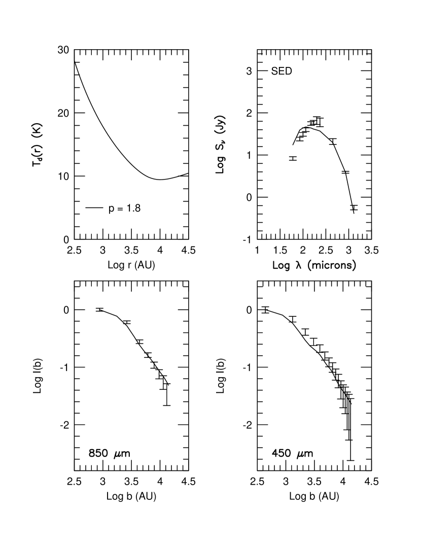
A power law is a good starting model because it has the same density distribution as a singular isothermal sphere, until it is truncated at an inner radius. The outer radius was chosen to allow proper simulation of chopping at the distance of B335 (250 pc; Tomita et al. 1979). The chop throw for our observations was 120″, corresponding to 30,000 AU at the distance of B335. Both the radial profile and the observed beam profile contain useful information 60″ from the center of the map; therefore, to allow the beam to chop onto the model density distribution for radial points 60″ from the center, the modelled density distribution must extend to twice the chop throw (240″) or 60,000 AU at the distance of B335. NICMOS observations of B335 indicate that reddening of background stars blend into the background noise beyond 125″ (Harvey et al. 2001), which is within the range of the outer radii tested in our models. We initially chose the inner radius such that so that AU for B335. For the initial test model, we used OH5 opacities. The fiducial density, , was varied to match the observed flux at 850 microns; , and the internal luminosity, , was varied until the model matched (Paper I). The resulting best fit was and (see Table 1). This basic model was used to test the effects of varying , , , , , and distance. The sensitivity of and to changes in the other parameters is summarized in Table 2.
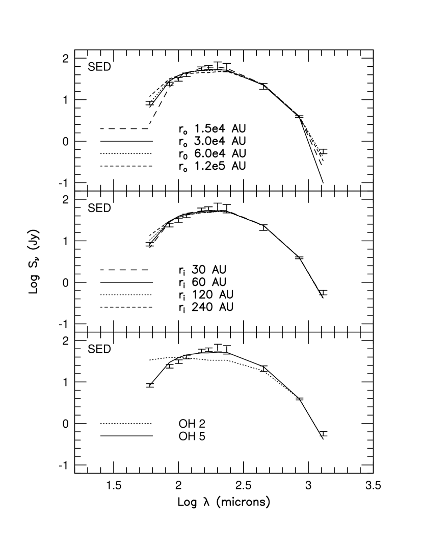
Changes in result in changes in the total envelope mass proportional to for a power law; however, the column density along a line of sight, and hence the emission at long wavelengths into a fixed beam becomes insensitive to for (). For the test model, the density is cm-3 at 60,000 AU. This low value is probably not realistic as the dense core is embedded in an extended cloud (Frerking et al. 1987). Even if a constant density of cm-3 is used for the lower limit to the density in the envelope, doubling the outer radius to 120,000 AU only increases AV by slightly less than 1 magnitude of visual extinction. This lower limit is used for all subsequent models. Allowing the density to fall below cm-3 results in no significant change in the best fit fiducial density or internal luminosity. Factor of two changes in have negligible effect on the best fit parameters. If is made small enough ( AU), the fit degrades (Table 1), but this is smaller than the extent of observed emission in the SCUBA map.
While the column density increases as decreases, beam dilution is more important. The SCUBA beams are much larger than the inner radii in our models (the 450 µm beamwidth of 8″ corresponds to a radius of 520 AU for our nearest source, B228); therefore changes in the inner radius will not have substantial effects unless the inner radius gets too large. Factor of two changes in have negligible effects; a factor of 4 increase in begins to degrade the fit to the 60 µm point on the SED (Figure 2). However, 60 µm observations can be affected by deviations from spherical geometry, so the 60 µm flux should not be considered a strong constraint on one dimensional models. We do not model the effects of a disk (see Section 5.5).
The result of these tests is that the best-fit model parameters are not sensitive to changes of factors of 2 in or . Larger changes worsen the fit, indicating that there is no evidence in our data for either inner or outer boundaries in the power laws.
Calculations of dust opacities differ substantially between dust models, especially at long wavelengths; for example OH5 and OH2 dust models have opacities at µm that are 6 and 12 times those of the model for dust in the diffuse interstellar medium (Draine & Lee 1984). With no further information, these differences would result in substantial uncertainties in , or equivalently the mass since . However, the SED is strongly affected by the choice of opacity law and can be used to distinguish dust models (e.g., Butner et al. 1991, van der Tak et al. 2000) if the density distribution is independently constrained. If OH2 opacities are used instead of OH5 opacities, the best fit power law remains with about one-third that of the test model. The higher (850) of OH2 dust requires less column density to match the flux at 850 µm. None of the power law fits using OH2 dust produce enough emission to match the SED at µm µm (Figure 2), yielding quite large values of . Changing the submillimeter opacity by a factor of a few does not strongly affect the shape of the model density profiles, confirming our conclusions about the orthogonality of the radial profile and the SED. A dust opacity that varies with radius could in principle affect the fit to the shape of the density profile; however, we see no evidence for variation of opacity with radius (see §5.3).
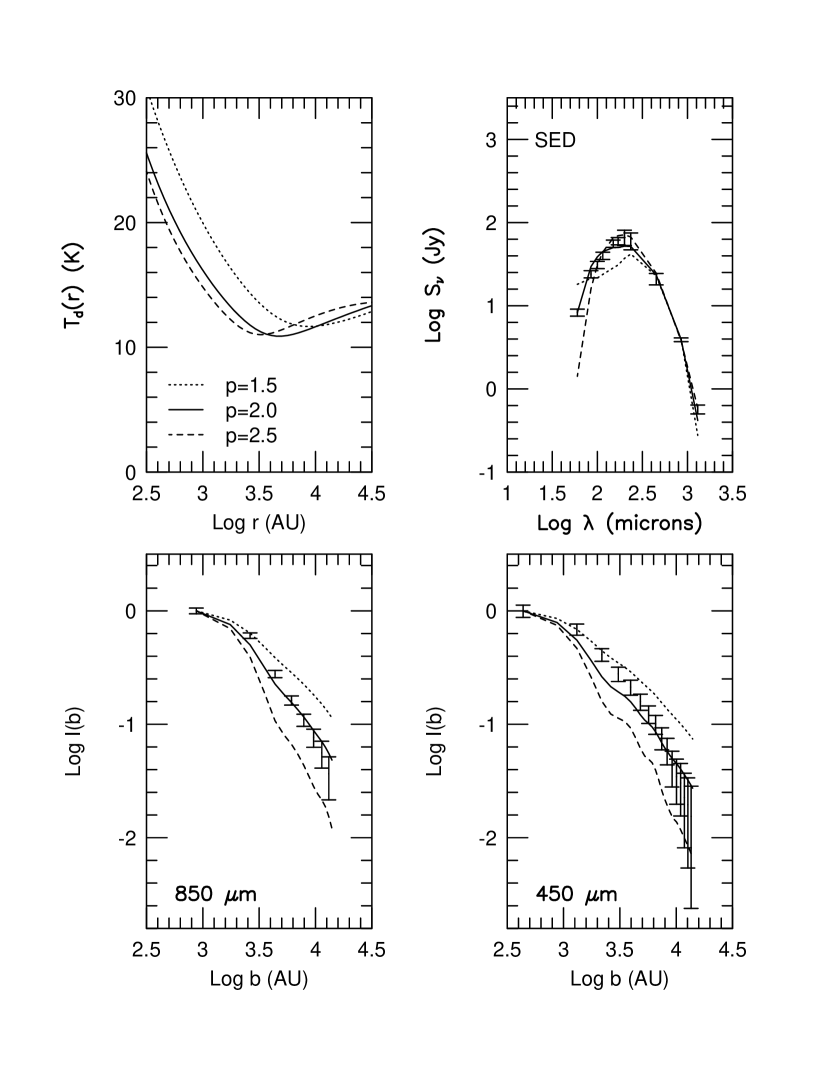
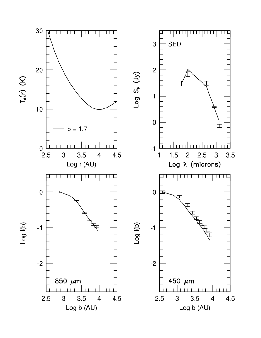
Other models of star formation predict density distributions different from the singular isothermal sphere (e.g. McLaughlin & Pudritz 1997, Ciolek & Basu 2000). Without explaining the details of these models we note that the differences often can be approximated by variations in the power law index () in the bulk of the envelope. We therefore considered models with , , and (Figure 3). Both the and models fit very poorly (Fig. 3). The model shows that the predicted radial profile becomes very sensitive to the beam shape for steep power laws. Variations in of 0.1 produce noticeable changes in the intensity profiles. In summary, we find that the initial test model is the best fit profile for OH5 dust and , and that variations in of 0.1 can be distinguished if all other parameters are fixed.
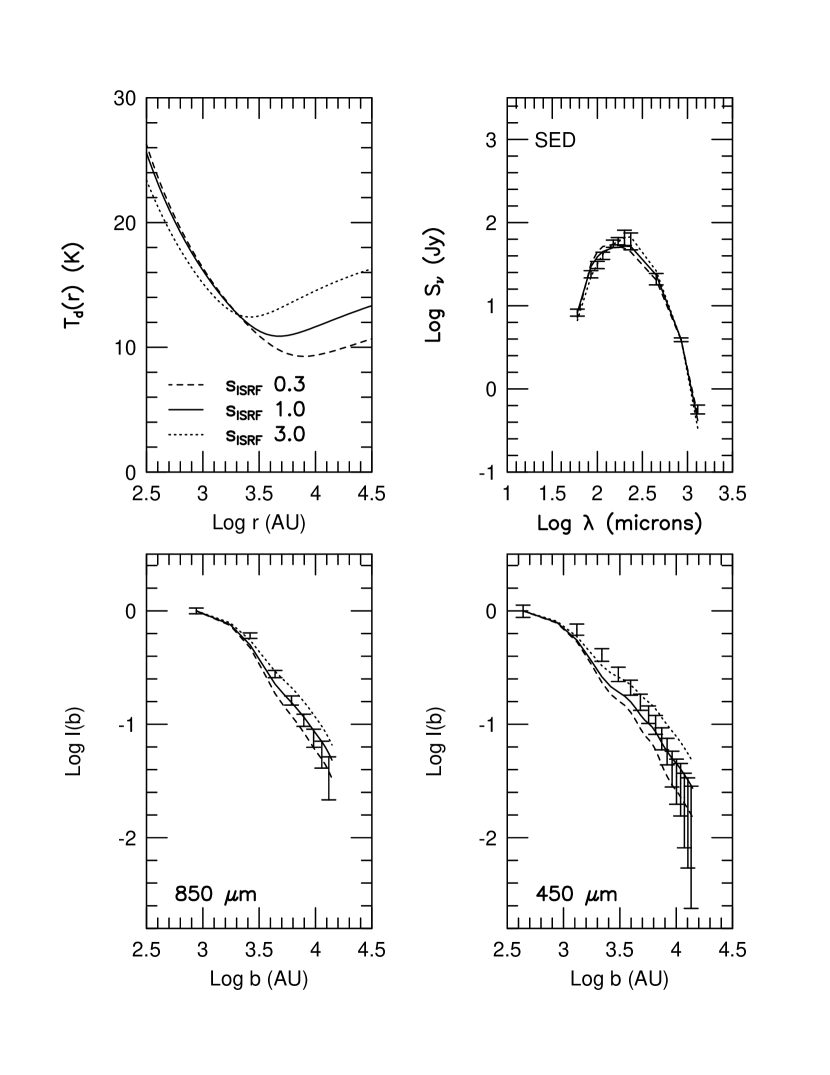
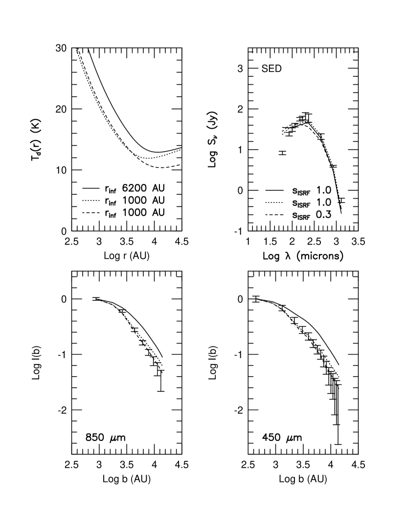
Heating by the ISRF affects the temperature distribution in the outer envelope. The temperature levels off and eventually rises again towards the outer boundary of the cloud. The location of the minimum in the temperature is dependent on the ISRF strength and (Figure 4). The strength of the ISRF could affect the intensity profiles and the SED. We tested these effects on the best fit power law by multiplying the ultraviolet to far-infrared portion of the ISRF by factors of and . With , the best fit is obtained with and L⊙. Obviously, the greater contribution to the flux from the ISRF explains why a lower internal luminosity is appropriate. Even though and are not significantly different from the standard model, the predicted SED is too bright at FIR wavelengths and severely underestimates the 60 µm flux. Using , the best fit is obtained with and (Figure 4 & 5). This model clearly yields the best fit to the intensity profiles of all of the power law models that we have considered, but the model SED has too much flux at shorter wavelengths (i.e., 60 µm). A lower strength of the ISRF is consistent with the best fit models in Paper II. A study of [CII] and [OI] emission lines with ISO towards B335 is consistent with a slightly higher strength of the ISRF, – (Nisini et al. 1999). Clearly, there is uncertainty in the strength of the ISRF around B335. We conclude that uncertainties of a factor of 10 in cause changes in by , but that the SED provides some constraints that can decrease this uncertainty.
The effect of the uncertainty in distance was checked on the initial test power law by assuming B335 was at half the published distance (125 pc; cf. Harvey et al. 2001). Since the core is now closer, smaller inner and outer radii (30 pc and 30,000 pc) were used. The best fit power law index and shape of the model profile are very insensitive to the uncertainty in the distance ( increases by less than ). The best fit L⊙, and the total mass in the model decreased by a factor of 2. The mass of a power law envelope scales as . For factor of 2 uncertainties in the distance, will be uncertain by factors of about 4, the mass by factors of 2 (for ), but the best fit is unaffected.
The effect of changing the observed beam shape was tested by substituting the January 1998 beamshape into the best fit power law model for B335. The difference in beamshape between January and April 1998 beams was greater than the difference between individual beam profiles observed during April 1998. The best fit power law was slightly lower, , indicating that uncertainties in the beam shape may effect the interpretation of the best fit model by as much as .
A power law with provides the best fit to the radial profiles for B335 (Figure 5). However, the is not as good for this model as for the test model. A somewhat different opacity law would fit better. The fit to the radial profiles is not perfect, with some systematic deviations as a function of impact parameter that suggest deviations from a simple power law, but given uncertainties in the beam shape, we consider this fit to be adequate.
In summary, our tests support the idea that the normalized radial profile () and the SED provide largely orthogonal constraints. constrains the shape () of the density profile, while (850) constrains the normalizing density, , and hence the mass. The density and mass enter as a product with the opacity at 850 µm, leading to uncertainties in the mass equal to the uncertainties in the opacities. However, the rest of the SED depends on the overall opacity law; within the limitations of spherical models, the overall SED constrains the opacity law and hence reduces the uncertainty in mass. Variations in other parameters, such as opacity, distance, and , have negligible effect on (Table 2). Variations in the ISRF have the largest effects: a factor of 3 in either direction in cause variations in of . Factors of 3 in can be constrained by the SED, so larger errors are unlikely. Opacity and the strength of the ISRF strongly affect (Table 2).
3.2 Shu77 Inside-Out Collapse Models
The Shu77 density distribution has successfully matched asymmetric line profiles seen towards Class 0 sources including B335 (Zhou et al. 1993, Choi et al. 1995, Hogerheijde et al. 2000). Based on Monte Carlo radiative transfer models of CS and H2CO asymmetric line profiles, Choi et al. found that a Shu77 model with AU and km s-1 was the best fit for an inside-out collapse model for B335. We mostly constrain to this value, unlike the procedure used by Hogerheijde & Sandell (2000), who allowed to be a free parameter. This lack of flexibility in the normalizing density puts Shu77 models at a disadvantage compared to the power law models with two free parameters.
The Shu77 density distribution with AU was tested assuming , and OH5 opacities. Compared to the best-fit power law model, the density in this Shu77 model is about 5 times less. There is simply not enough material to match the SED: had to be increased to L⊙ to match because the lower optical depths allowed too much radiation at µm, which is not observed. Even with the large , the fits to both the SED and radial profiles are extremely poor (Figure 6). The model radial profiles are too flat. This is not surprising since a power law model did not fit the observed radial profiles.
Shu77 models would need smaller infall radii to preserve an density distribution throughout a greater extent of the envelope. Smaller infall radii provide better fits to the radial profile. The best of these models, with AU and , has a very good . However, AU is less than the FWHM of the SCUBA beam at 450 µm. Thus, the best fit Shu77 model actually resembles a power law in all portions of the profile except the central beam. A small infall radius is highly unfavored by models of profiles of molecular lines ( is 20 times worse, Choi et al 1995). Further radiative transfer modeling of the molecular line emission using the best fit density profiles from the dust models and considering possible abundance variations in the molecular tracers may resolve this discrepancy.
Thus, the Choi et al. model has two problems: the density is too low to match the observed SED, and the density distribution is not steep enough to match . Because other opacity models combined with Shu77 models have fit the SED of B335 (Zhou et al. 1990), the first problem is not necessarily fatal. The bigger problem is the failure to match .
The near infrared extinction study of Harvey et al. (2001) found that the Choi et al. (1995) parameters for a Shu77 model did fit the density structure of the outer envelope, but require a scaling of the density by a factor of 5. Such a large increase would require a higher or B335 to be much closer. A higher is not supported by the narrow linewidth observed towards B335 (e.g., Mardones et al. 1997). As shown in the power law models of B335, a closer distance does not strongly affect the interpretation of the best fit radial profiles; therefore, an infall radius of AU would still not fit the observed normalized intensity profile. This solution, which worked for Harvey et al., does not work for our data. A small infall radius would be required to match the SCUBA profiles with a Shu77 model. The increased density required by Harvey et al. (2001) to model their near-infrared extinction measurements makes their densities agree well with our best-fit power law model, which is based on OH5 opacities at 850 µm. The OH5 opacity at 850 µm and the extinction used by Harvey et al. in the near-infrared thus produce consistent density estimates. This agreement supports the validity of OH5 dust, as does our comparison of dust and virial masses (§5.2).
4 Sources
The other sources were modeled with less extensive exploration of parameter space, guided by the results of the B335 models.
4.1 B228
B228 is a deeply embedded protostar (IRAS 15398-3359) which appears very similar to B335 at 850 and 450 µm. The B228 contours are nearly circularly symmetric with extended envelope emission and a high signal-to-noise profile. Unlike B335, B228 is much less studied and therefore has less published SED information (see Paper I). B228 is an excellent candidate for 1D dust modeling of the envelope emission and should be the subject of further detailed study. We shall try both power law and Shu77 models.
A range of power law indices were tried with noticeable changes in the with changes of . The best fit power law is with a lower ISRF () and an internal luminosity of 1.0 L⊙ (see Figure 7). Since B228 is closer than B335 (130 pc, see Paper I), the outer radius was decreased to 30,000 AU. While the power law is a reasonable fit to both the profile and SED, it has the same problem as the B335 power law fits. The model profile is too steep in the inner portion of the envelope and too shallow in the outer portion of the profile. The deviations may be due to subtle changes in the beam shape or to departures from a single power law. Far-infrared photometry with better spatial resolution and more wavelength points would help to constrain the SED.
The best fit Shu77 collapse model has an infall radius of AU and an effective sound speed of km s-1. The linewidth of optically thin lines in B228 (e.g., (N2H+) in Mardones et al 1997) is similar to that of lines in B335. Therefore an km s-1 is reasonable. As with B335, the infall radius is within the central SCUBA beam. The best fit Shu77 model was able to simultaneously match the observed bolometric luminosity and the flux at 850 µm. The fit to the profiles are not as good as the fit of the best fit power law, and is considerably worse.
4.2 L723
The submillimeter emission from L723 (IRAS 19156+1906) has asymmetries only in the lowest contours of the 850 and 450 µm emission. The higher contours are very circularly symmetric. A quadrupolar outflow has been detected, indicating that L723 may contain a close binary (Palacios & Eiroa, 1999) within a common envelope. Alternatively, the outflow may be due to a single source with a very large opening angle (Hirano et al. 1998). The largest extensions in the lowest contours of the SCUBA maps are roughly aligned with an east-west outflow. The unique characteristics of the outflow structure and the possibility that L723 may be a proto-binary system warrant a detailed study of the dust continuum structure of the envelope.
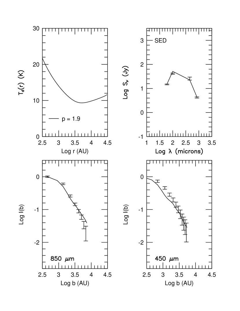
L723 is best fitted by a power law with (Figure 8). The fit to the profiles and SED is very good using OH5 dust. The model internal luminosity is L⊙ indicating a contribution of L⊙ to the bolometric luminosity from the ISRF. The large contribution from the ISRF may be due to the large size of model ( AU) and the greater distance ( pc; Goldsmith et al. 1984) of L723. Emission was detected beyond 65″ ( AU) in the 850µm SCUBA map, larger than the outer radius quoted by Motte & André (2001) of AU from 1.3 mm continuum maps. As seen in the test models of B335, decreasing the outer radius to AU has a negligible effect on the shape of the radial profile and the interpretation of the best fit power law.
The best fit power law is very similar to the other circularly symmetric cores B335 and B228. While L723 may be a proto-binary system, there is no strong evidence for differences in the one dimensional dust models of L723 and B335 or B228. Multiple dimensional dust models are needed to probe the extended structure at low contour levels in the SCUBA maps. The envelope structure of L723 is complicated by the extensive observed outflows. The impact the outflow structure has on the overall distribution of material in the envelope cannot be effectively modeled with only one spatial dimension.
The best fit Shu77 model has a small infall radius ( AU) and effective sound speed of km s-1. The fit to the profile and SED is very good. As with B335 and B228, the infall radius is within the central 450 µm SCUBA beam. There is no evidence for a break in the power law density distribution in the outer envelope beyond the central beam.
4.3 IRAS03282+3035
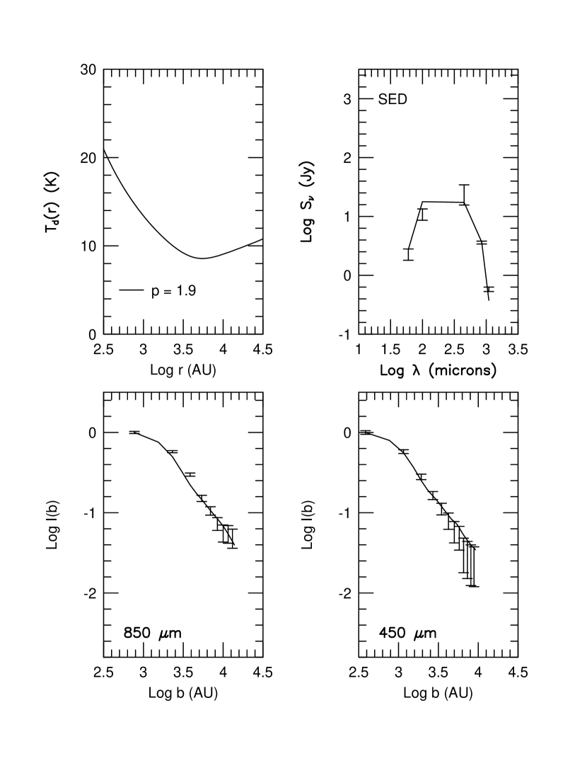
IRAS 03282+3035 is a nearly circular symmetric core with slight asymmetries in the lowest contour of the 850 and 450 µm emission. There is a well studied outflow (e.g., Bachiller et al. 1994) that is nearly perpendicular to the extended submillimeter continuum emission. The signal-to-noise of the radial profiles was lower for this object (Paper I).
The best fit to IRAS 03282+3035 is a power law with lower strength of the ISRF, (see Figure 9). The model fits the 850 µm profile marginally better than the 450 µm profile. Since IRAS 03282+3035 was observed during January 1998, the beam profile is much more uncertain, resulting in larger uncertainties in the best fit model. L⊙ for the best fit model, accounting for nearly all of the bolometric luminosity.
We continue to use a distance of pc (Černis 1990) for consistency with Paper I, but the recent study of de Zeeuw et al. (1999) finds a greater distance of pc using Hipparcos parallaxes of the Perseus OB association. At the larger distance, the internal luminosity and mass in the envelope would increase by a factor of two. As was seen in the models of B335, the best fit power law index is not sensitive to distance and remains .
The best fit Shu77 model again has a infall radius of AU within the central SCUBA beam. Molecular line observations towards IRAS03282+3035 indicate linewidths that are similar to B228 and B335 (N2H km s-1, Mardones et al. 1997); however, a higher effective sound speed ( km s-1) than used for B228 is needed to match the 850 µm flux and simultaneously using OH5 dust.
4.4 L1448C
L1448C (also called L1448-mm) is a well studied Class 0 protostar in the vicinity of 3 other deeply embedded protostars in the Perseus molecular cloud (L1448N(A & B), L1448NW; see O’Linger et al. 1999, Barsony et al. 1998). L1448C drives a powerful, highly collimated outflow (Bachiller et al. 1990) for which proper motion has been detected in extremely high velocity SiO maps (Girat & Acord 2001). H2O maser emission has been detected (Chernin 1995) indicating the presence of very dense gas. Recently, the infrared spectrum from 6µm to 190µm has been observed with ISO and extensively studied (Giannini et al. 2001, Nisini et al. 1999). As for IRAS03282+3035, we continue to use a distance of 220 pc, but 318 pc is more likely (de Zeeuw et al. 1999); the effects on the model parameters are described in the previous section.
The submillimeter contours are circularly symmetric with a weak bridge of emission extending between L1448C and L1448N/L1448NW (Barsony et al. 1998, Chandler & Richer 2000, Paper I). L1448C is located 82″ from the nearest source (L1448N); therefore we shall attempt to model L1448C as an isolated source with the strong caveat that the outer portion of the observed radial profile (i.e., ″) is contaminated with emission from L1448N and L1448NW. Only points in the radial profile ″ from L1448C are modeled.
The best fit power law was with (Figure 10). An outer radius of AU was used for the best fit model. This model cannot be compared directly to observations beyond half the distance between L1448C and L1448N/L1448NW ( AU projected on the sky). However, the large outer radius is appropriate for the model since all of the sources in the SCUBA map are clearly embedded in a diffuse envelope that extends to the edge of the map. The model of the 450 µm profile falls off too steeply for the best-fit 850 µm profile, which could be caused by a larger or uncertainties in the beam.
This power law density structure is slightly flatter than that of the other protostars with symmetric submillimeter emission. If the entire profile of L1448C is contaminated from emission from L1448N/L1448NW, then the observed intensity profile would be flatter than for an isolated source resulting in a flatter best fit . However, it seems unlikely that the northern sources could significantly alter the conclusions of the modeling of the entire profile since they are located at least AU away.
This is the only modeled source for which gave the best fit. This source is also the only source modeled with multiple cores observed within the SCUBA map. It is possible that this indicates that the ISRF is indeed greater in the vicinity of L1448C; however, the overall change in the between and is only .
4.5 L1527
L1527 is a well studied Class 0 source (IRAS 04368+2557) in the Taurus molecular cloud complex characterized by asymmetric submillimeter and far-infrared emission extending from the southeast to northwest direction (Ladd et al. 1991, Chandler & Richer 2000, Hogerheijde & Sandell 2000, Paper I, Motte & André 2001), strong evidence for rotation (Goodman et al. 1993, Zhou et al. 1996, Ohashi et al 1997), a molecular outflow in the east-west direction (MacLeod et al. 1994, Bontemps et al. 1996), and an associated near-infrared nebula (Eiroa et al. 1994). The normalized radial intensity profile was not well fitted by a single power law in Paper I, as it shows considerable curvature. Previous studies of the dust continuum emission (Hogerheijde & Sandell 2000, Motte & André 2001) have estimated the density power law to be near , much lower than the best fit power laws of B335 and B228.
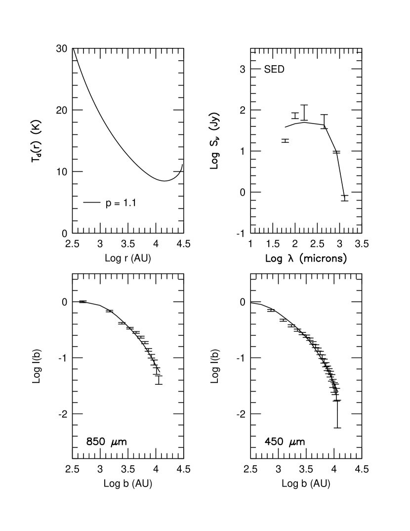
The best fit power law model (see Figure 11) is a shallow power law with , in agreement with previous dust continuum studies of L1527. The fit to the 850 µm profile is within the errorbars except for the last point. The observed profile is slightly flatter than the model power law between 5000 and 6500 AU. The 450 µm model profile is flatter than the observed profile in the inner portion but matches extremely well in the outer envelope. These discrepancies may be explained by the inability of the one-dimensional dust code to appropriately model the observed large asymmetries in the dust continuum maps or may be explained by the problematic January 1998 beam profiles (cf. Section 2). The beam effects cannot be strong enough to change our conclusion that the density structure in L1527 is clearly flatter than the density structure of B335 or B228. The curvature in can be matched by simple power laws when and the effects of the beam and chopping are properly simulated. The fit to the SED is poor at far-infrared wavelength as indicated by the the poor for all of the models in Table 1.
The sensitivity of the model to asymmetries can be tested by eliminating sectors in the azimuthally averaged intensity profile. L1527 is elongated in a south-east to north-west direction. If a symmetrical sector of 70∘ centered along the major axis is removed from the azimuthal average, then the best fit power law index changes only to . Therefore, the density distribution appears to fall off more slowly even perpendicular to the extension; thus the lower value of appears to be real and not an artifact of azimuthally averaging an elongated intensity map. Uncertainties on the order of result from azimuthally averaging the L1527 continuum emission. The uncertainty in best fit is consistent with effects seen in 1.3mm continuum maps of L1527 (Motte & André 2001).
A standard Shu collapse model was not tested since the density distribution only flattens to in a small region around the infall radius and is much steeper everywhere else in the envelope. Zhou et al. (1996) were able to model molecular line emission with a Terebey-Shu-Cassen model (TSC, Terebey et al. 1984), a perturbation of the Shu collapse model to account for rotation. The one-dimensional averaged TSC profile is similar to in the region inside the infall radius (5400 AU). A more detailed understanding of the density structure requires higher dimensional radiative transfer models to effectively model the asymmetric, flattened structure due to rotation and outflow cavities.
4.6 L483
L483 (IRAS 18148-0440) is another example of a Class 0 protostar with large asymmetries observed in the submillimeter continuum maps. The 850 and 450 µm emission is extended in the northeast to southwest direction (Paper I), nearly perpendicular to the observed outflow direction (Parker 1988). Water maser emission has been detected towards L483 (Xiang & Turner 1992) as well as an associated near-infrared nebula (Hodapp 1994). Molecular line studies identify this source as a possible collapse candidate (Mardones et al. 1997) but with several confusing signatures due to infall and outflow (Park et al. 2001).
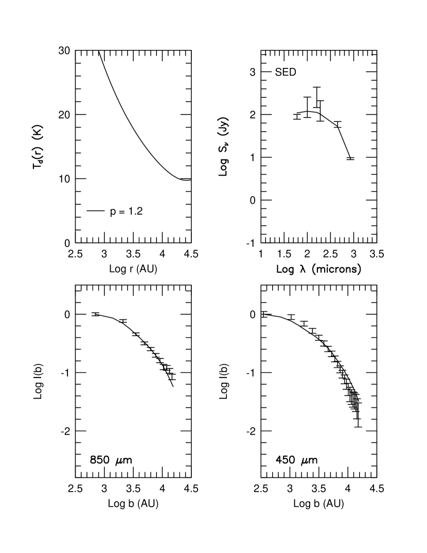
The dust continuum emission from L483 is best fitted by a shallow () power law with (Figure 12). The model SED and 850 µm radial profile match very well but the 450 µm model profile is not steep enough in the outer half of the envelope. This may be partially due to uncertainties in the beam profile at 450 µm, a variation in the dust opacity in the outer envelope, or a variation in the temperature structure due to geometrical effects compared to a one dimensional model. Once again, OH5 dust matches the observed SED well; however, the 160 µm point from Ladd et al. (1991) is much higher than the surrounding 100 µm and 190 µm points, perhaps indicating a larger calibration error than the published value. The internal luminosity of the model is L⊙. This is the most luminous source in this sample of Class 0 objects, making the contribution to the bolometric luminosity from the ISRF negligible compared to the internal luminosity, but the effects on the temperature profile are still substantial. The resulting temperature profile flattens near the outer regions probed by SCUBA observations making a single temperature power law a poor approximation. Our model is consistent with mm continuum models of Motte & André (2001), which assume a power law temperature distribution, , ( for ). The best fit model becomes optically thick around 30 µm due to the flatter power law and higher luminosity internal source.
Like L1527, the L483 profiles were not well fitted by a single power law in Paper I, but a power law density distribution does fit well when the beam, chopping, and are correctly modeled. The best fit power law is close to , for both these sources with elongated dust emission contours. Both L1527 and L483 have near-infrared nebulae associated with the core. However, both cores are not entirely similar since the extensions seen in the submillimeter continuum contours are in opposite directions with respect to the outflow axes. Geometrical projection effects are clearly important for these two sources. Tafalla at al. (2000) and Pezzuto et al. (2001) suggest this source is in the transitional phase between Class 0 and Class I sources based on the observed properties of its outflow and far-infrared colors. While still a Class 0, it does have the largest (52K) of the sources we model here. While the envelope structure is clearly different from the more symmetrical cores B335 and B228, it is not clear whether the lower indicates a more evolved state or an intially less spherical envelope. Higher dimensional dust modeling is required to fully understand the density structure of the outer envelope.
No Shu collapse models were tested since the power law model was flatter than the Shu collapse model. However, it is possible that a higher dimensional model that includes effects of rotation (TSC) may fit the intensity profile.
5 Discussion
5.1 Density Distributions
The properties of the best fit power law for all of the Class 0 sources are listed in Table 4. Power law models successfully fit the outer ( AU) envelope structures of Class 0 protostars. Five of the Class 0 sources are well fitted by steep power laws (, B335, B228, L723, IRAS03282+3035, L1448C), while the two cores with elongated emission contours are fitted by shallow power laws (, L1527, L483). We quantify the degree of elongation in Table 4 by giving the aspect ratio (ratio of long axis to short axis) of the 20% contour. L1527 and L483 have the largest aspect ratios. Both L1527 and L483 also have near-infrared nebulae, suggestive of aspherical density distributions. The fiducial densities for all of the Class 0 cores are consistent with the central densities ( cm-3) of the denser pre-protostellar cores modeled as Bonnor-Ebert spheres in Paper II.
The best fit Shu77 models for B335, B228, L723, and IRAS03282+3035 have small infall radii (within the central SCUBA beam). The Shu77 models look very similar to the best fit power laws, but generally do not fit as well. There is no strong evidence in the radial profiles for a break in slope indicative of an infall radius in the outer portion of the envelope probed by SCUBA. This result directly contradicts the molecular line modeling results towards B335 (Choi et al. 1995), which strongly favors larger infall radii. However, the molecular line models do not take into account chemical effects and abundance gradients, which can affect the shape of the blue asymmetry profile (Rawlings & Yates 2001). Unfortunately, the best fit power laws cannot be directly used in Monte Carlo molecular line modeling without an assumption about the velocity field along the line of sight.
5.2 Mass Determinations
The mass in the envelope within a 120″ aperture was calculated using
| (6) |
The average mass is M⊙ for the seven Class 0 best fit power laws, times higher than the average pre-protostellar core mass ( M⊙) within the same aperture (cf. Paper II). The average mass within a fixed outer radius of AU is M⊙ for Class 0 sources compared to M⊙ for pre-protostellar cores. If these Class 0 sources are the next stage of evolution, they clearly have most of their mass in the envelope, as originally proposed by Andrè et al. (1993).
In the absence of a realistic model for , masses are usually determined from submillimeter observations using an isothermal approximation. To facilitate mass determinations for sources without models, we explored the most suitable temperature to use. We calculated the isothermal dust temperature that yields the same mass as the detailed model based on the measured 850 µm flux in a 120″ beam, , using
| (7) |
The results are listed in Table 4. Most are 11-13 K, but the most luminous source, L483, has K. L1448C is excluded due to confusion from the northern sources in the 120″ aperture. The mean value is K. The sources with (L1527, L483) have higher (K and K respectively). A similar calculation can be made for the pre-protostellar cores modeled in Paper II using the mass of a Bonnor-Ebert sphere within the 120″ aperture. For the three pre-protostellar cores, the average isothermal temperature is ( K L1544, K L1689B, K L1512), slightly lower than for Class 0 sources with an internal luminosity source.
The model dust mass can be compared to the virial mass calculated using optically thin linewidths (e.g., N2H+ and H13CO+; see Table 8 in Paper I). The virial mass estimates in Paper I assumed a constant density distribution in the envelope; however, the virial mass can be corrected for the best fit power law density distribution (cf. Bertoldi & McKee 1992) using
| (8) |
where is the FWHM size of the aperture in which the dust mass was determined, is the distance, and is the 3-D velocity dispersion:
| (9) |
where is the FWHM linewidth of an optically thin line, is the mean molecular mass, and is the molecular mass of the species whose linewidth is used.
The mean of the ratio of the virial mass to the model dust mass in a 120″ aperture is . Uncertainties of up to a factor of in the opacity exist between different dust models (Ossenkopf & Henning 1994). We regard this agreement as encouraging evidence that OH5 opacities describe the dust in the cores well and that the virial theorem, properly applied, gives good mass estimates. This ratio is also consistent with the ratio of virial mass to model dust mass for a sample of deeply embedded high mass star forming cores associated with water masers (, Evans et al. 2002). A factor of decrease in from the OH5 value would bring the dust model mass and virial mass into agreement on average.
5.3 Spectral Indices
The spectral index, , was calculated from the model fluxes at 450 and 850 µm in a 120″ aperture (L1448C excluded due to confusion) using
| (10) |
The model spectral index calculated within a 120″ aperture agrees extremely well with the observed spectral index from Paper I; . The model spectral indices are within the observed error bars; however, the total uncertainty on the 450 µm flux () makes the observed spectral index fairly uncertain. OH5 opacities are also successful in reproducing the observed submillimeter spectral indices for Class 0 sources.
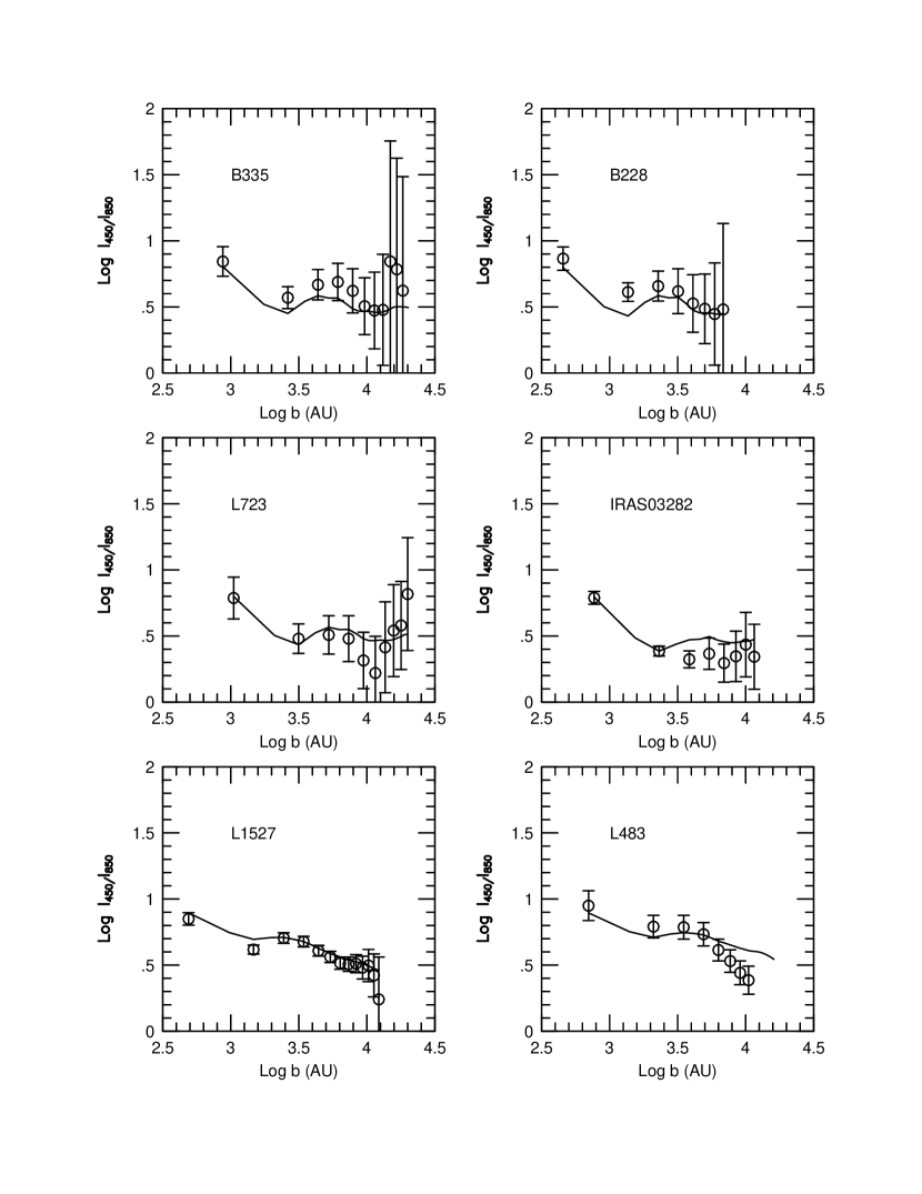
We also considered possible changes in the spectral index as a function of impact parameter. To avoid calibration uncertainties we compare the normalized specific intensity, , for the best fit models to the observed ratios (Figure 13). The variations in the model ratio match those in the observed ratio. Apparent variations in the spectral index can be removed by taking into account beam effects and a realistic temperature distribution. For example, the first sidelobe at 450µm results in a large increase in the ratio. The lower signal-to-noise in outer annuli would mask any subtle variations in the dust opacity. L483 is a clear exception as the model specific intensity ratio does not decrease as fast as the observed ratio. The 450 µm model is too flat at large radii. However, this discrepancy may be caused by our use of a spherical model on an aspherical source rather than an actual variation in the dust properties. There is thus little evidence for variations of the dust opacity with radius. This result contrasts with some earlier work (e.g., Visser et al. 1998, Johnstone & Bally 1999) in regions forming more massive stars, but agrees with the conclusions of Chandler & Richer (2000), who were studying regions similar to those in this study. It is extremely important to use a realistic beam profile and for modeling both the 850 and 450 µm SCUBA maps.
5.4 The ISRF and
The contribution from the ISRF can be important to the heating of the region of the outer envelope probed by SCUBA observations of low luminosity cores. Scaling the ultraviolet to far-infrared portion of the ISRF by a factor of 3 in either direction resulted in changes of the best fit power by factors of . Every source profile except L1448C was better fitted by a lower strength of the ISRF, , in agreement with models of pre-protostellar cores (Paper II). Modest shielding of the ISRF by surrounding gas in the molecular cloud surrounding the dense core could account for this. L1448C is forming in a much more crowded region and may be subjected to a stronger ISRF.
Our models provide an estimate of the internal luminosity of the central protostar. For all of our sources, the internal luminosity accounts for nearly all of the observed luminosity (). While the heating from the ISRF is important for the temperature structure of the outer envelope, it does not contribute significantly to the overall observed luminosity of the Class 0 sources we modeled. There is a wide range of internal luminosities modeled, from L⊙ to L⊙, with an average internal luminosity of L⊙. For each of the best fit models, the flux at 850 µm and the observed bolometric luminosity were fitted simultaneously. For sources with SEDs not observed shortward of 60 µm, the model internal luminosity is a lower limit. All of the luminosities were calculated using the distances from Paper I. Since the distance to many globules are uncertain to 50%, a true determination of the internal luminosity is uncertain to 100%; however, the model and observed internal luminosities are consistent for the distance adopted.
Interestingly, the most luminous source, L483, has about the same envelope mass as the others. The greater luminosity should reflect either a higher stellar mass or a higher accretion rate. If the former, it would imply a higher starting mass for the condensation; if the latter, it might be reflected in the linewidths. In fact, the linewidth of the N2H+ line is similar to that of the other sources. Alternatively, the accretion might be in a transient high state, similar to an FU Orionis event.
5.5 Caveats and Future Work
While our models take into account heating from a central source, heating from the ISRF, realistic beam effects, and simulated chopping, they cannot effectively model asymmetries seen in the dust continuum maps, flattening due to rotation or effects of magnetic fields, and clearing of material in outflow cavities. Five of the cores modeled (B335, B228, L723, IRAS03282+3035, L1448C) appear sufficiently symmetric that the most important effect not included would be lower densities in outflow cavities. Harvey et al. (2001) found a strong asymmetry in the (H – K) colors along the outflow directions in B335, indicative of clearing of material along the outflow axes. The resulting best fit models included an outflow opening angle of 35∘ to 45∘. While no such asymmetry is observed in the submillimeter continuum maps of B335 (Paper I), extensions along the outflow directions (e.g., L1527, L723) and perpendicular to the outflow direction (e.g., L483) are observed in submillimeter maps of Class 0 sources. The overall impact outflows have on the density structure of the envelope will become clearer with finer resolution and higher sensitivity. Future multi-dimensional modeling of the dust continuum emission should attempt to account for the effects of the outflow.
We have neglected the emission from a disk. Chandler & Richer (2002) showed that the flux from a disk is negligible compared to the the total flux from the envelope of Class 0 sources; however, Class 0 sources may have a substantial fraction of emission from a compact component within the central beam. The interpretation of the density structure of the outer envelope may be strongly affected when a centrally normalized radial profile is used. Only a few Class 0 sources have been observed at submillimeter wavelengths with interferometers (cf. Brown et al. 2000) resulting in few constraints on submillimeter disk fluxes. Observations of 2.7mm continuum towards L1527 with OVRO and BIMA find a flux of mJy from a compact component (Terebey et al. 1994, Shirley et al. unpublished observation). Using a model for an active disk (; Butner et al. 1994), we find an upper limit of Jy at 850 µm. In this scenario, the disk accounts for up to of the flux within the central beam, decreasing by . It is likely that the 7″ aperture included flux from the envelope, thereby overestimating the flux from a disk. If the disk has a steeper temperature power law (), then the flux contribution drops to Jy at 850 µm and the change in the best fit power law model is . As another example, the Choi et al. (1996) Shu77 model fits the B335 radial profile when the disk flux equals the envelope flux within the central beam ( Jy at 850 µm). However, BIMA millimeter observations of B335 do not support such a high disk flux (Shirley et al., unpublished observation). Constraints on the disk flux and modeling of BIMA observations of the dust continuum towards Class 0 protostars will be presented in a future paper.
6 Conclusions
We have modeled seven Class 0 sources using single power law and Shu77 density distributions. Power law models suitably fit the 850 µm profiles and SED of all Class 0 sources. Five sources with circular contours are best fitted by a steep value of the power law index (B335, B228, L723, IRAS03282+3035, L1448C), while two sources with aspherical emission are fitted by flatter power law indices (L1527, L483). Uncertainties in the strength of the ISRF, , and beam shape limit the accuracy in the power law index to .
The Shu77 model from Choi et al. (1995) does not fit the B335 radial profiles. Smaller infall radii are able to fit the profiles (B335, B228, L723, IRAS03282+3035, L1448C), but the infall radius is within the central 450 µm beam, effectively making the density distribution appear like a single power law throughout the region of the envelope probed by SCUBA.
The average mass within a 120″ aperture is M⊙ and is reasonably consistent with virial mass estimates and observed mass estimates from Paper I and models of the initial conditions from Paper I. We find little evidence for variations in the dust opacity with radius. OH5 dust reproduces the observed spectral index on average and provides a good fit to many SEDs. In addition, it leads to masses determined from dust emission that are consistent with virial masses to a factor of 2. Heating from the ISRF is very important for correctly interpreting the temperature profile of the outer envelope of low mass star forming cores but does not significantly contribute to the total bolometric luminosity. The dust models constrain the internal luminosity of Class 0 protostars, but distances to isolated cores remain the largest uncertainty in determining accurate masses and luminosities.
Outflow cavities and asymmetrical density distributions should be modeled using higher dimensional dust modeling. In particular, L483 and L1527 have large asymmetries in the dust continuum emission that cannot be modeled with a one dimensional code.
The presence of a disk within the central beam may affect the interpretation of the best fit density distribution in the outer envelope, decreasing by as much as .
We can now use a more realistic and in Monte Carlo molecular line radiative transfer models to test infall models (which provide ) and the origin of line asymmetries, to test predictions of chemical models, to investigate amounts of depletion, and to improve estimates of the ionization fraction.
Our primary conclusion is that a simple power law for the density distribution fits all of the Class 0 sources that we have considered, while Shu77 models with substantial do not fit. Firmer conclusions await stronger constraints on the submillimeter flux from a possible disk and modeling of interferometric observations of Class 0 protostars.
Acknowledgments
We are grateful to L. Mundy for providing the computer code used for beam convolution and solution of Equation (1) and for stimulating discussions about the effects of disk. We thank Steve Doty for useful discussions and consistency checks of our 1D models. We thank Chad Young for his help simulating effects of a disk. We are grateful to the referee, Antonella Natta, who made many helpful suggestions. We thank the State of Texas and NASA (Grants NAG5-7203 and NAG5-10488) for support. NJE thanks the Fulbright Program and PPARC for support while at University College London and NWO and NOVA for support in Leiden. The JCMT is operated by the Joint Astronomy Centre on behalf of the Particle Physics and Astronomy Research Council of the United Kingdom, The Netherlands Organization for Scientific Research and the National Research Council of Canada.
References
- (1)
- (2) Adams, F. C. 1991, ApJ, 382, 544
- (3) Alves, J. F., Lada, C. J., & Lada, E. A. 2001, Nature, 409, 159
- (4) André, P., Ward-Thompson, D., & Barsony, M. 1993, ApJ, 406, 122
- (5) André, P., Ward-Thompson, D., & Barsony, M. 2000, in Protostars and Planets IV, ed. Mannings, V., Boss, A. P., & Russell, S. S. (Tucson:University of Arizona Press)
- (6) Bachiller, R., Chernicharo, J., Martin-Pintado, J., Tafalla, M., & Lazareff, B. 1990, A&A, 231, 74
- (7) Bachiller, R., Terebey, S., Jarrett, T., Martin-Pintado, J., Beichman, C. A., & van Buren, D. 1994, ApJ, 437, 296
- (8) Barsony, M. Ward-Thompson, D. Andre,́ P., & OĹinger, J. 1998, ApJ, 509, 733
- (9) Bertoldi, F., & McKee, C. F. 1992, ApJ, 395, 140
- (10) Black, J. H. 1994, ASP Conf. Ser. 58: The First Symposium on the Infrared Cirrus and Diffuse Interstellar Clouds, 355
- (11) Bontemps, S., Andre, P., Terebey, S. & Cabrit, S. 1996, A&A, 311, 858
- (12) Brown, D. W., Chandler, C. J., Carlstrom, J. E., Hills, R. E., Lay, O. P., Matthews, B. C., Richer, J. S., & Wilson, C. D. 2000, MNRAS, 319, 154
- (13) Butner, H. M., Natta, A., & Evans, N. J., II 1994, ApJ, 420, 326
- (14) Butner, H. M., Evans, N. J., II, Harvey, P. M., Mundy, L. G., Natta, A., & Randich, M. S. 1990, ApJ, 364, 164.
- (15) Butner, H. M., Evans, N. J., II, Lester, D. F., Levreault, R. M., & Strom, S. E. 1991, ApJ, 376, 636
- (16) Černis, K. 1990, Ap&SS, 166, 315
- (17) Chandler, C. J., & Richer, J. S. 2000, ApJ, 530, 851
- (18) Chen, H., Myers, P. C., Ladd, E. F., & Wood, D. O. S. 1995, ApJ, 445, 377
- (19) Chernin, L. M. 1995, ApJL , 400, L97
- (20) Ciolek, G. E., & Basu, S. 2000, ApJ, 529, 925
- (21) Draine, B. T., & Lee, H. M. 1984, ApJ, 285, 89
- (22) Egan, M. P., Leung, C. M., & Spagna, G. R. 1988, Comput. Phys. Comm., 48, 271
- (23) Eiroa, C., Miranda, L. F., Anglada, G., Estalella, R., & Torrelles, J. M. 1994, A&A, 283, 973.
- (24) Evans, N. J., Rawlings, J. M. C., Shirley, Y. L., & Mundy, L. G. 2001, ApJ, 557, 193
- (25) Evans, N. J., Shirley, Y. L., Mueller, K. M., & Knez, C. 2002, in Hot Star Workshop III: The Earliest Phases of Massive Star Birth, ASP Conference Series, Vol. xxx, 2002, ed. P. A. Crowther
- (26) Frerking, M. A., Langer, W. D., & Wilson, R. W. 1987, ApJ, 313, 320
- (27) Galli D., & Shu F. 1993, ApJ, 417, 220
- (28) Galli D., & Shu F. 1993, ApJ, 417, 243
- (29) Giannini, T., Nisini, B., & Lorenzetti, D. 2001, ApJ, 555, 40
- (30) Girart, J. M., Acord, J.M.P. 2001, ApJL, 551, L63
- (31) Goldmsith, P. F., Snell, R. L., Hemeon-Heyer, M., & Langer, W. D. 1984, ApJ, 286, 599
- (32) Goodman, A. A., Benson, P. J., Fuller, G. A., & Myers, P. C. 1993, ApJ, 406,528
- (33) Harvey, D.W.A., Wilner, D. J., Lada, C. J., Myers, P. C., Alves, J. F., & Chen, H. 2001, preprint
- (34) Hirano, N., Hayashi, S. S., Umemoto, T., & Ukita, N. 1998, ApJ, 504, 334
- (35) Hodapp, K.-W., 1994, ApJS, 94, 615
- (36) Hogerheijde, M. R., & Sandell G. 2000, ApJ, 534, 880
- (37) Holland et al. 1999, MNRAS 303, 659
- (38) Hollenbach, D. J., Takahashi, T., & Tielens, A. G. G. M. 1991, ApJ, 377, 192
- (39) Huard, T. L., Sandell, G., & Weintraub, D. A. 1999, ApJ, 526, 833
- (40) Johnstone, D. & Bally, J. 1999, ApJ, 510, L49
- (41) Lada, C. J. 1987, in IAU Symp. 115, Star Formation Regions, ed. M. Peimbert & J. Jugaku (Dordrecht:Reidel), 1
- (42) Ladd, E. F., et al. 1991, 382, 555
- (43) Mathis, J. S., Mezger, P. G., & Panagia, N. 1983, A&A, 128, 212
- (44) MacLeod, J., Avery, L., Harris, A., Tacconi, L. & Schuster, K. 1994, JCMT Newsletter No. 3, 46
- (45) McLaughlin, D. E., & Pudritz, R. E. 1997, ApJ, 476, 750
- (46) Motte, F., André P. 2001, A&A, 365, 440
- (47) Nisini, B., et al. 1999, A&A, 350, 529
- (48) Ohashi, N., Hayashi, M., Ho, P. T. P., Momose, M., Tamura, M., Hirano, N., Sargent, A. I. 1997, ApJ, 488, 317
- (49) OĹinger, J., Grace, W-C., Barsony, M., & Ward-Thompson, D. 1999, ApJ, 515, 696
- (50) Ossenkopf, V., & Henning, Th. 1994, A & A, 291, 943
- (51) Palacios, J., & Eiroa, C. 1999, A&A, 346, 233
- (52) Park, Y.-S., Panis, J.-F., Ohashi, N., Choi, M., & Minh, Y. C. 2001, 542, 344
- (53) Parker, N. D., Padman, R., Scott, P. F., & Hills, R. E. 1988, MNRAS, 234, 67
- (54) Pezutto, S. et al. 2001, accepted in MNRAS, (astroph/0111270)
- (55) Rawlings, J.M.C., & Yates, J.A. 2001, MNRAS, 326, 1423
- (56) Shirley, Y. L., Evans, N. J. E., Rawlings, J. M. C., & Gregersen, E. M. 2000, ApJS, 131, 249
- (57) Shu, F. H. 1977, ApJ, 214, 488
- (58) Terebey, S. Chandler, C. J., & André, P. 1993, ApJ, 414, 759
- (59) Terebey, S., Shu F. H., & Cassen, P. 1984, ApJ, 286. 529
- (60) Tomita, Y., Saito, T., & Ohtani, H. 1979, PASJ, 31, 407
- (61) van der Tak, F. S., van Dishoeck, Ewine F., Evans II, N. J., & Blake, G. A. 2000, ApJ, 537, 283
- (62) van Dishoeck, E. F. 1988, Rate Coefficients in Astrochemistry, T. J. Millar and D. A. Williams, Dordrect: Kluwer, 49
- (63) Visser, A. E., Richer, J. S., Chandler, C. J., & Padman, R. 1998, MNRAS, 301, 585
- (64) Visser, A. E., Richer, J. S., & Chandler C. J. 2001, MNRAS, accepted
- (65) Walker, C. K., Adams, F. C., & Lada, C. J., 1990, ApJ, 349, 515
- (66) Xiang, D.-L., Turner, B. E. 1992, AcASn, 33, 87
- (67) Zhou, S. 1995, ApJ, 442, 685
- (68) Zhou, S., Evans, N. J., Koempe, C., & Walmsley, C. M. 1993, ApJ, 404, 232
- (69) Zhou, S., Evans, N. J., & Wang, Y. 1996, ApJ, 466, 296
- (70)

| Source | aa calculated using all flux points listed in Tables 5, 6, and 7 of Shirley et al. 2000 with . | Notes | |||||||||
|---|---|---|---|---|---|---|---|---|---|---|---|
| (cm-3) | (AU) | (AU) | (L⊙) | ||||||||
| B335 | |||||||||||
| 2.0 | 60 | 60,000 | OH5 | 2.5 | 1.0 | 5.9 | 3.9 | 2.2 | Test Model | ||
| 2.0 | 30 | 60,000 | OH5 | 2.5 | 1.0 | 6.8 | 5.0 | 2.1 | |||
| 2.0 | 120 | 60,000 | OH5 | 2.5 | 1.0 | 5.4 | 3.4 | 2.7 | |||
| 2.0 | 240 | 60,000 | OH5 | 2.7 | 1.0 | 4.4 | 2.1 | 5.9 | |||
| 2.0 | 60 | 120,000 | OH5 | 2.5 | 1.0 | 5.0 | 3.5 | 5.7 | |||
| 2.0 | 60 | 30,000 | OH5 | 2.5 | 1.0 | 6.5 | 3.8 | 5.8 | |||
| 2.0 | 60 | 15,000 | OH5 | 2.5 | 1.0 | 16.9 | 10.8 | 7.3 | |||
| 1.8 | 60 | 15,000 | OH5 | 2.5 | 1.0 | 5.4 | 3.9 | 5.8 | |||
| 1.5 | 60 | 60,000 | OH5 | 2.8 | 1.0 | 79.4 | 34.5 | 22.6 | |||
| 2.5 | 60 | 60,000 | OH5 | 2.5 | 1.0 | 47.1 | 19.7 | 8.5 | |||
| 2.0 | 60 | 60,000 | OH5 | 1.5 | 3.0 | 14.7 | 9.5 | 1.7 | |||
| 2.2 | 60 | 60,000 | OH5 | 1.5 | 3.0 | 5.6 | 3.4 | 5.6 | |||
| 2.0 | 60 | 60,000 | OH5 | 3.0 | 0.3 | 12.2 | 8.9 | 4.2 | |||
| 1.8 | 60 | 60,000 | OH5 | 3.3 | 0.3 | 3.8 | 2.9 | 19.6 | Best | ||
| 2.0 | 60 | 60,000 | OH2 | 4.4 | 1.0 | 6.2 | 3.8 | 101 | |||
| B228 | |||||||||||
| 2.1 | 60 | 30,000 | OH5 | 1.0 | 1.0 | 11.4 | 8.6 | 30.7 | |||
| 1.9 | 60 | 30,000 | OH5 | 1.0 | 0.3 | 8.8 | 6.4 | 4.8 | Best | ||
| L723 | |||||||||||
| 2.0 | 60 | 60,000 | OH5 | 2.0 | 1.0 | 1.1 | 1.3 | 9.6 | |||
| 1.8 | 60 | 60,000 | OH5 | 2.6 | 0.3 | 0.8 | 0.5 | 3.4 | Best | ||
| 1.8 | 60 | 30,000 | OH5 | 2.6 | 0.3 | 0.8 | 0.6 | 3.7 | |||
| IRAS03282bbIRAS03282+3035. | |||||||||||
| 2.1 | 60 | 45,000 | OH5 | 1.0 | 1.0 | 13.5 | 3.5 | 4.6 | |||
| 1.9 | 60 | 45,000 | OH5 | 1.0 | 0.3 | 10.2 | 1.2 | 5.2 | Best | ||
| L1448C | |||||||||||
| 1.7 | 60 | 45,000 | OH5 | 5.9 | 1.0 | 4.7 | 10.4 | 2.0 | Best | ||
| 1.6 | 60 | 45,000 | OH5 | 5.9 | 0.3 | 8.3 | 9.4 | 9.3 | |||
| L1527 | |||||||||||
| 1.5 | 60 | 30,000 | OH5 | 1.8 | 1.0 | 76.7 | 39.6 | 13.7 | |||
| 1.0 | 60 | 30,000 | OH5 | 2.1 | 1.0 | 52.3 | 60.3 | 25.6 | |||
| 1.1 | 60 | 30,000 | OH5 | 2.2 | 0.3 | 9.2 | 5.4 | 28.3 | Best | ||
| L483 | |||||||||||
| 1.3 | 60 | 45,000 | OH5 | 13.0 | 1.0 | 8.9 | 5.1 | 1.2 | |||
| 1.2 | 60 | 45,000 | OH5 | 13.0 | 0.3 | 6.1 | 5.2 | 1.0 | Best |
| Variable | RangebbThe range of the variable tested. | ||
| (L⊙) | |||
| – AU | |||
| – AU | |||
| – cm-3 | |||
| – L⊙ | … | ||
| OH5 vs. OH2 | |||
| – | |||
| ccThe beam shape. | Jan. vs. Apr. | ||
| … |
| Source | Notes | ||||||||||
|---|---|---|---|---|---|---|---|---|---|---|---|
| (AU) | (km/s) | (cm-3) | (AU) | (AU) | (L⊙) | ||||||
| B335 | |||||||||||
| 6200 | 0.23 | 60 | 60,000 | OH5 | 6.5 | 1.0 | 79.0 | 53.7 | 108 aaUnable to simultaneously match and . | ||
| 6200 | 0.26 | 60 | 60,000 | OH5 | 5.0 | 1.0 | 82.1 | 52.8 | 62.2 | ||
| 1000 | 0.23 | 60 | 60,000 | OH5 | 3.8 | 1.0 | 7.6 | 3.6 | 36.7 | ||
| 500 | 0.23 | 60 | 60,000 | OH5 | 3.0 | 1.0 | 9.0 | 3.5 | 15.8 | ||
| 1000 | 0.23 | 60 | 60,000 | OH5 | 4.5 | 0.3 | 2.3 | 0.8 | 66.8 aaUnable to simultaneously match and . | Best | |
| 1000 | 0.26 | 60 | 60,000 | OH5 | 4.0 | 0.3 | 2.4 | 1.0 | 39.1 | ||
| 6200 | 0.23 | 60 | 60,000 | OH2 | 6.5 | 0.3 | 39.6 | 21.9 | 59.0 aaUnable to simultaneously match and . | ||
| 1000 | 0.23 | 60 | 60,000 | OH2 | 4.7 | 0.3 | 2.6 | 1.1 | 58.8 aaUnable to simultaneously match and . | ||
| B228 | |||||||||||
| 1000 | 0.23 | 60 | 30,000 | OH5 | 1.0 | 0.3 | 2.9 | 15.6 | 32.2 | Best | |
| L723 | |||||||||||
| 1000 | 0.29 | 60 | 60,000 | OH5 | 2.6 | 0.3 | 1.1 | 0.6 | 2.49 | Best | |
| IRAS03282bbIRAS03282+3035. | |||||||||||
| 1000 | 0.23 | 60 | 45,000 | OH5 | 1.0 | 0.3 | 4.8 | 13.3 | 34.1 aaUnable to simultaneously match and . | ||
| 1000 | 0.26 | 60 | 45,000 | OH5 | 1.0 | 0.3 | 3.9 | 9.5 | 18.7 | Best | |
| L1448C | |||||||||||
| 1500 | 0.38 | 60 | 45,000 | OH5 | 5.9 | 1.0 | 10.5 | 3.0 | 2.4 |
| Source | AspectaaRatio of major to minor axis for the 20% peak contour. | |||||||||
|---|---|---|---|---|---|---|---|---|---|---|
| Ratio | ||||||||||
| (cm-3) | (L⊙) | (L⊙) | (L⊙) | (M⊙) | (K) | M⊙ | ||||
| B335 | 1.8 | 3.1(0.1) | 3.3 | 3.1 | 2.5 | 2.6 | 1.08 | 13.2 | 4.8 | |
| B228 | 1.9 | 1.2(0.2) | 1.0 | 1.1 | 2.6 | 0.8 | 1.22 | 12.5 | 2.8 | |
| L723 | 1.8 | 3.3(0.2) | 2.6 | 3.4 | 2.5 | 3.9 | 1.42 | 12.4 | 7.7 | |
| IRAS03282bbIRAS03282+3035. | 1.9 | 1.2(0.3) | 1.0 | 1.2 | 2.4 | 2.4 | 1.03 | 11.5 | 3.6 | |
| L1448CccQuantities calculated using a 120″ aperture not shown due to confusion from nearby sources. | 1.7 | 6.0(0.5) | 5.9 | 6.0 | … | 4.5 | … | … | … | |
| L1527 | 1.1 | 2.2(0.2) | 2.2 | 2.2 | 2.4 | 1.6 | 1.59 | 15.0 | 2.6 | |
| L483 | 1.2 | 13(2) | 13.0 | 12.9 | 2.7 | 2.3 | 1.93 | 18.0 | 5.4 |