FIRST ATTEMPT AT MEASURING THE CMB CROSS-POLARIZATION

Abstract

We compute upper limits on CMB cross-polarization by cross-correlating the PIQUE and Saskatoon experiments. We also discuss theoretical and practical issues relevant to measuring cross-polarization and illustrate them with simulations of the upcoming ${\rm BOOMERanG}$ 2002 experiment. We present a method that separates all six polarization power spectra (TT, EE, BB, TE, TB, EB) without any other “leakage” than the familiar EE-BB mixing caused by incomplete sky coverage. Since E and B get mixed, one might expect leakage between TE and TB, between EE and EB and between BB and EB — our method eliminates this by preserving the parity symmetry under which TB and EB are odd and the other four power spectra are even.

]

I INTRODUCTION

Although not yet detected, it is theoretically expected that the Cosmic Microwave Background (CMB) is polarized. CMB polarization should be induced via Thomson scattering which occurs either at decoupling or during reionization. The level of this polarization is linked to the local quadrupole anisotropy of the incident radiation on the scattering electrons, and it is expected to be of order 1%-10% of the amplitude of the temperature anisotropies depending on the angular scale (see [1, 2] and references therein).

CMB polarization is important for two reasons: first, polarization measurements can substantially improve the accuracy with which cosmological parameters are measured by breaking the degeneracy between certain parameter combinations; second, it offers an independent test of the basic assumptions that underly the standard cosmological model.

Since the polarized CMB signal is so small, it is quite likely that its first detection will be an indirect statistical one, from its predicted correlation with an unpolarized CMB map. Since such cross-correlations involve one rather than two powers of the (small) polarization fraction, they will be measured with better signal-to-noise than polarization autocorrelations. Indeed, it has been shown [3, 4] that for almost all cosmological parameters, the polarization capabilities of upcoming high-precision CMB experiments such as MAP and Planck add information mainly through the cross-polarization signal, the only exceptions being the reionization and gravity wave parameters.

The goal of the present paper is to present a detailed study of the cross-polarization from a practical point of view, connecting real-world data to physical models. In section Section II, we argue that the dimensionless correlation coefficient $r_{\l}$ is a more meaningful quantity to discuss than the cross power spectrum $C_{\l}^{X}$, and illustrate how it depends of various cosmological parameters for standard adiabatic models.

In Section III, we compute the strongest observational constraints to date on $r_{\l}$ by cross-correlating the polarized Princeton IQU Experiment (PIQUE) [5] with the unpolarized Saskatoon (SK) [6] data set. We do this using the formalism presented in [7], which takes into account real–world issues such as incomplete sky coverage and correlated noise. Finally, in Section IV we assess the prospects for measuring $r_{\l}$ in the near future by analyzing a simulated version of the upcoming ${\rm BOOMERanG}$ 2002 experiment.

II POLARIZATION PHENOMENOLOGY

Whereas most astronomers use the Stokes parameters $Q$ and $U$ to describe polarization measurements, the CMB community uses two scalar fields $E$ and $B$ that are independent of how the coordinate system is oriented, and are related to the tensor field $(Q,U)$ by a non–local transformation [8, 9, 10]. Scalar CMB fluctuations have been shown to generate only $E$-fluctuations, whereas gravity waves, CMB lensing and foregrounds generate both $E$ and $B$. This formalism has been applied to real data by the PIQUE [5] and POLAR [11] teams.

A The six power spectra

Since CMB measurements can be decomposed into three maps ($T$,$E$,$B$), where $T$ denotes the unpolarized component, there are a total of 6 angular power spectra that can be measured. We will denote these $C_{\l}^{T}$, $C_{\l}^{E}$, $C_{\l}^{B}$, $C_{\l}^{X}$, $C_{\l}^{Y}$ and $C_{\l}^{Z}$, corresponding to $TT$, $EE$, $BB$, $TE$, $TB$ and $EB$ correlations, respectively. By parity, $C_{\l}^{Y}=C_{\l}^{Z}=0$ for scalar CMB fluctuations, but it is nonetheless worthwhile to measure these power spectra as probes of both exotic physics [16, 17, 18] and foreground contamination. $C_{\l}^{B}=0$ for scalar CMB fluctuations to first order in perturbation theory [8, 9, 10, 19] — secondary effects such as gravitational lensing can create $B$ polarization even if there are only density perturbations present [20]. The remaining three power spectra are plotted in Figure 1 (top) for the “concordance” model of [21] (that of [22] is very similar), showing that $C_{\l}^{E}$ is typically a couple of orders of magnitude below $C_{\l}^{T}$ on small scales and approaches zero on the very largest scales (in the absence of reionization).

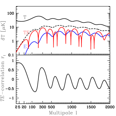
FIG. 1.: The $T$, $X$ and $E$ power spectra are shown (top panel) for the concordance model of [21]. The $TE$ correlation coefficient $r^{X}_{\l}$ (bottom panel) is the ratio between $C_{\l}^{X}$ and the geometric mean of $C_{\l}^{T}$ and $C_{\l}^{E}$, so in the top panel, $|r^{X}_{\l}|$ is just the distance between $TE$ and the geometric average of the $T$ and $E$ curves (dashed curve).

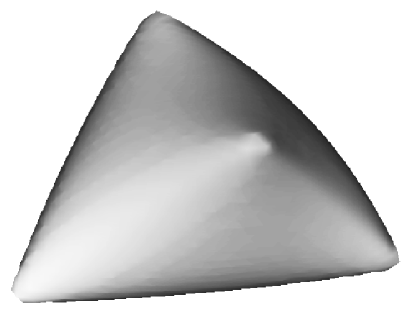
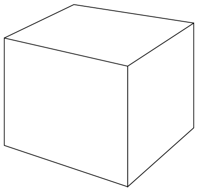
FIG. 2.: The region of the parameter space $(r^{X},r^{Y},r^{Z})$ allowed by the generalized Schwarz inequality. The cube extends from $-1$ to $1$ in all three dimensions. The four corners $(1,1,1)$, $(1,-1,-1)$, $(-1,1,-1)$ and $(-1,-1,1)$ correspond to $T$, $E$ and $B$ being perfectly correlated and anticorrelated.

B Covariance versus correlation

The cross-power spectrum $C_{\l}^{X}$ is not well suited for such a logarithmic plot, since it is negative for about half of all $\l$-values. A more convenient quantity is the dimensionless correlation coefficient $r^{X}_{\l}$ plotted in Figure 1 (lower panel), defined as

$$r^{X}_{\l}\equiv{C_{\l}^{X}\over(C_{\l}^{T}C_{\l}^{E})^{1/2}},$$ (1)

since the Schwarz inequality restricts it to lie in the range

$$-1\leq r^{X}_{\l}\leq 1.$$ (2)

These dimensionless correlations/anticorrelations are seen to be quite strong in the sense of being near these limiting values on many scales. For instance, if one were to smooth the $T$- and $E$-maps to contain only large angular scales $\l\mathrel{\hbox to0.0pt{\lower 3.0pt\hbox{$\mathchar 536\relax$}\hss}\raise 2.0pt\hbox{$\mathchar 316\relax$}}10$ where $r^{X}_{\l}\sim 0.9$, they would be so strongly correlated that most hot and cold spots would tend to line up. Conversely, if one were to band-pass filter the two maps on scales $100\mathrel{\hbox to0.0pt{\lower 3.0pt\hbox{$\mathchar 536\relax$}\hss}\raise 2.0pt\hbox{$\mathchar 316\relax$}}\l\mathrel{\hbox to0.0pt{\lower 3.0pt\hbox{$\mathchar 536\relax$}\hss}\raise 2.0pt\hbox{$\mathchar 316\relax$}}200$ where $r^{X}_{\l}\mathrel{\hbox to0.0pt{\lower 3.0pt\hbox{$\mathchar 536\relax$}\hss}\raise 2.0pt\hbox{$\mathchar 316\relax$}}-0.6$, hot spots in the $T$-map would tend to line up with cold spots in the $E$-map.

More generally, let us also define $r^{Y}_{\l}$ $\equiv$ $C_{\l}^{Y}/(C_{\l}^{T}C_{\l}^{B})^{1/2}$, $r^{Z}_{\l}$ $\equiv$ $C_{\l}^{Z}/(C_{\l}^{E}C_{\l}^{B})^{1/2}$. Expanding the $T$, $E$ and $B$ maps in spherical harmonics with coefficients $a_{\l m}^{T}$, $a_{\l m}^{E}$ and $a_{\l m}^{B}$, the three cross power spectra are by definition the covariances $C_{\l}^{X}=\langle a_{\l m}^{T*}a_{\l m}^{E}\rangle$, $C_{\l}^{Y}=\langle a_{\l m}^{T*}a_{\l m}^{B}\rangle$, $C_{\l}^{Z}=\langle a_{\l m}^{E*}a_{\l m}^{B}\rangle$, so $r^{X}$, $r^{Y}$ and $r^{Z}$ are simply the correlation coefficients between $a_{\l m}^{T}$, $a_{\l m}^{E}$ and $a_{\l m}^{B}$.

What values are these three correlation coefficients allowed to take? They are real-valued just as $T$, $E$ and $B$, which is most easily seen using real-valued spherical harmonics. The dimensionless correlation matrix corresponding to the vector $(a_{\l m}^{T},a_{\l m}^{E},a_{\l m}^{B})$ is

$${\bf R}=\left(\begin{tabular}[]{ccc}1&$r^{X}_{\l}$&$r^{Y}_{\l}$\\ $r^{X}_{\l}$&1&$r^{Z}_{\l}$\\ $r^{Y}_{\l}$&$r^{Z}_{\l}$&1\\ \end{tabular}\right),$$ (3)

and by virtue of being a correlation matrix, it cannot have any negative eigenvalues. This implies not only that $|r^{X}_{\l}|\leq 1$, $|r^{Y}_{\l}|\leq 1$ and $|r^{Z}_{\l}|\leq 1$, but also that the determinant of ${\bf R}$ must be non-negative, i.e., that

$$(r^{X}_{\l})^{2}+(r^{Y}_{\l})^{2}+(r^{Z}_{\l})^{2}-2r^{X}_{\l}r^{Y}_{\l}r^{Z}_{\l}\leq 1$$ (4)

for all $\l$. This allowed region in the 3-dimensional space $(r^{X},r^{Y},r^{Z})$ is plotted in Figure 2, and is seen to resemble a deformed tetrahedron. If two coefficients are strongly correlated with each other, then they must both have roughly the same correlations with the third, approaching the limiting case $(r^{X},r^{Y},r^{Z})=(1,1,1)$ (upper right corner). The other three corners correspond to the allowed possibilities $(1,-1,-1)$, $(-1,1,-1)$ and $(-1,-1,1)$.

From here on we use $r_{\l}$ as shorthand for $r^{X}_{\l}$.

C Cosmological parameter dependence of polarization power spectra

A detailed review of how CMB polarization reflects underlying physical processes in given in [2]. In this subsection, we briefly review this topic from a more phenomenological point of view (see also [12]), focusing on how different cosmological parameters affect various features in the $E$, $B$ and $X$ power spectra and aiming to familiarize the reader with, in particular, the correlation spectrum $r_{\l}$ and its cosmology dependence. For more details, the reader is refererred to the polarization movies at www.hep.upenn.edu/$\sim$angelica/polarization.html.

Let us consider adiabatic inflationary models specified by the following 10 parameters: the reionization optical depth $\tau$, the primordial amplitudes $A_{s}$, $A_{t}$ and tilts $n_{s}$, $n_{t}$ of scalar and tensor fluctuations, and five parameters specifying the cosmic matter budget. The various contributions $\Omega_{i}$ to critical density are for curvature $\Omega_{\rm k}$, vacuum energy $\Omega_{\Lambda}$, cold dark matter $\Omega_{\rm cdm}$, hot dark matter (neutrinos) $\Omega_{\nu}$ and baryons $\Omega_{\rm b}$. The quantities $\omega_{\rm b}\equiv h^{2}\Omega_{\rm b}$ and $\omega_{\rm dm}\equiv h^{2}\Omega_{\rm dm}$ correspond to the physical densities of baryons and total (cold + hot) dark matter ($\Omega_{\rm dm}\equiv\Omega_{\rm cdm}+\Omega_{\nu}$), and $f_{\nu}\equiv\Omega_{\nu}/\Omega_{\rm dm}$ is the fraction of the dark matter that is hot. The baseline values of the parameters here and in the movies are for the concordance model of [21], $\tau=\Omega_{\rm k}=A_{t}=f_{\nu}=0$, $\Omega_{\Lambda}=0.66$, $\omega_{\rm dm}=0.12$, $\omega_{\rm b}=0.02$, $n_{s}=0.93$, providing a good fit to current data from the CMB, galaxy and Lyman Alpha Forest clustering and Big Bang nucleosynthesis.

1 Polarized versus unpolarized

If recombination were instantaneous, there would be no polarization at all!

Both the $E$ and the $T$ power spectra carry information about the $z\mathrel{\hbox to0.0pt{\lower 3.0pt\hbox{$\mathchar 536\relax$}\hss}\raise 2.0pt\hbox{$\mathchar 318\relax$}}10^{3}$ pre-recombination epoch in the form of acoustic oscillations. From a practical point of view, there are two obvious differences between the $E$ and $T$ power spectra as illustrated by Figure 1:

• The $E$ power is smaller since the polarization percentage is small, making measurements more challenging. This is because polarization is only generated when locally anisotropic radiation scatters off of free electrons, and this only occurs during the brief period when recombination is taking place: before recombination, radiation is quite isotropic and after recombination there is almost no scattering.

• Aside from reionization effects, the $E$ power approaches zero on scales much larger than those of the first acoustic peak. This is because the polarization anisotropies are only generated on scales of order the mean free path at recombination and below.

As detailed below, changing the cosmological parameters affects the polarized and unpolarized power spectra rather similarly except for the cases of reionization and gravity waves. All power spectra were computed with the CMBfast software [25].

2 Reionization

Reionization at redshift $z_{*}$ introduces a new scale $\l_{*}\sim 20(z_{*}/10)^{1/2}$ corresponding to the horizon size at the time. Primary (from $z\mathrel{\hbox to0.0pt{\lower 3.0pt\hbox{$\mathchar 536\relax$}\hss}\raise 2.0pt\hbox{$\mathchar 318\relax$}}1000$) fluctuations $\delta T_{\l}$ on scales $\l\gg\l_{*}$ get suppressed by a factor $e^{\tau}$ and new series of peaks are generated starting at the scale $\l_{*}$. Figure 3 illustrates that although these new peaks are almost undetectable in $T$, drowning in sample variance from the unpolarized Sachs-Wolfe effect, the are clearly visible in

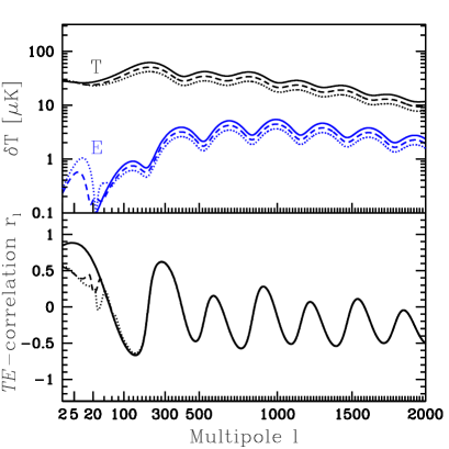
FIG. 3.: How the reionization optical depth $\tau$ affects the $T$ and $E$ power spectra (top) and the $TE$ correlation $r_{\l}$ (bottom). Solid, dashed and dotted curves correspond to for $\tau$=0, 0.2 and 0.4, respectively.

$E$ since the Sachs-Wolfe nuisance is unpolarized and absent. The models in Figure 3 have abrupt reionization giving $\tau\propto z_{*}^{3/2}$, so higher $z_{*}$ is seen to shift the new peaks both up and to the right.

On small scales, reionization leaves the correlation $r_{\l}$ unchanged since $C_{\l}^{T}$ and $C_{\l}^{E}$ are merely rescaled. On very large scales, $r_{\l}$ drops since the new polarized signal is uncorrelated with the old unpolarized Sachs-Wolfe signal. On intermediate scales $\l\mathrel{\hbox to0.0pt{\lower 3.0pt\hbox{$\mathchar 536\relax$}\hss}\raise 2.0pt\hbox{$\mathchar 318\relax$}}\l_{*}\sim 20$, oscillatory correlation behavior is revealed for the new peaks.

For more details about CMB polarization and reionization see [26].

3 Primordial perturbations

As seen in Figure 4, gravity waves (a.k.a. tensor fluctuations) contribute only to fairly large angular scales, producing $E$ and $B$ polarization. Just as for the reionization case, unpolarized fluctuations are also produced but are difficult to detect since they get swamped by the Sachs-Wolfe effect. As has been frequently pointed out in the literature, no other physical effects (except CMB lensing and foregrounds) should produce $B$ polarization, potentially making this a smoking gun signal of gravity waves.

Adding a small gravity wave component is seen to suppress the correlation $r_{\l}$ in Figure 4, since this component is uncorrelated with the dominant signal that was there previously. Indeed, this large-scale correlation suppression may prove to be a smoking gun signature of gravity waves that is easier to observe in practice than the oft-discussed  $B$-signal.  This  $TE$-correlation  suppression

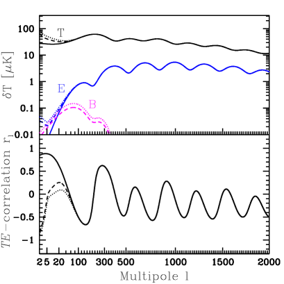
FIG. 4.: How the gravity wave amplitude $A_{t}$ affects the $T$, $E$ and $B$ power spectra (top) and the $TE$ correlation $r_{\l}$ (bottom). Solid, dashed and dotted curves correspond to for $A_{t}$=0, 0.2 and 0.4, respectively.

comes mainly from $E$, not $T$: since the tensor polarization has a redder slope than the scalar polarization, it can dominate $E$ at low $\l$ even while remaining subdominant in $T$.

The amplitudes $A_{s}$, $A_{t}$ and tilts $n_{s}$, $n_{t}$ of primordial scalar and tensor fluctuations simply change the amplitudes and slopes of the various power spectra: B is controlled by $(A_{t},n_{t})$ alone, whereas $T$ and $E$ are affected by $(A_{s},n_{s})$ and $(A_{t},n_{t})$ in combination. Note that if there are no gravity waves ($A_{t}=0$), then these amplitudes and tilts cancel out, leaving the correlation spectrum $r_{\l}$ independent of both $A_{s}$ and (apart from aliasing effects) $n_{s}$.

4 Spacetime geometry

Just as $A_{s}$ and $n_{s}$, the spacetime geometry parameters $\Omega_{\rm k}$ and $\Omega_{\Lambda}$ affect the polarized and unpolarized power spectra in similar ways. $\Omega_{\rm k}$ and $\Omega_{\Lambda}$ were completely irrelevant at $z>10^{3}$, when the acoustic oscillations were created, since $\Omega_{\rm k}\approx\Omega_{\Lambda}\approx 0$ at that time regardless of their present values. As is well-known and illustrated by the above-mentioned movies, the acoustic peak features are therefore independent of these parameters, merely shifting sideways on a logarithmic plot as geometric effects magnify/shrink the scale of primordial fluctuation patterns. On large scales, the late ISW effect creates additional power that is completely unpolarized, since this is a pure gravity effect involving no Thomson scattering. Since the ISW effect is uncorrelated with the primary large-scale fluctuations, it suppresses $r_{\l}$ on large scales as $\Omega_{\rm k}$ or $\Omega_{\Lambda}$ shift away from zero as seen in Figure 5.

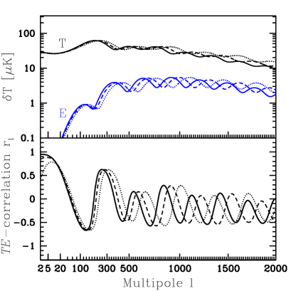
FIG. 5.: How the spatial curvature $\Omega_{\rm k}$ affects the $T$ and $E$ power spectra (top) and the $TE$ correlation $r_{\l}$ (bottom). Solid, dashed and dotted curves correspond to $\Omega_{\rm k}=-0.1$ (closed model), $0$ (flat model) and $0.1$ (open model), respectively. Apart from the familiar horizontal shift, the late ISW effect is seen to suppress the correlation $r_{\l}$ on large scales.

5 Matter budget

The Primordial CMB signal is dominated by fluctuations in the gravitational potential and the density at $z\sim 10^{3}$, whereas the $E$-signal is dominated by peculiar velocities on the last scattering surface. This is why the $E$-spectrum is seen to be out of phase with the T-spectrum, peaks in one matching troughs in the other. This also explains why increasing the baryon fraction $f_{b}\equiv\Omega_{\rm b}/(\Omega_{\rm b}+\Omega_{\rm dm})$ as in Figure 6 lowers the polarized peaks, in contrast to the boosting of odd peaks for the unpolarized case: more baryons lower the sound speed in the photon-baryon plasma, producing lower velocities.

The remaining matter budget parameters, the cold and hot dark matter densities, effect $E$ polarization in much the same way $T$. Increasing the dark matter density $h^{2}\Omega_{\rm dm}$ shifts the peaks down and to the left. The $T$, $E$ and $r_{\ell}$ power spectra change hardly at all when changing the fraction $\Omega_{\nu}/\Omega_{\rm dm}$ of the dark matter that is hot. This is because the neutrinos were already quite cold (nonrelativistic) at the time the CMB fluctuations are formed.

III Case study I: PIQUE

We now turn to the issue of measuring cross-polarization in practice, including issues of methodology, window functions and leakage. We analyze an existing data set in this section, then turn to simulations of upcoming data in Section IV .

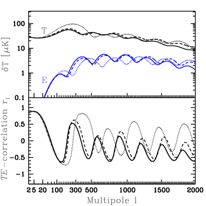
FIG. 6.: How the baryon fraction $\Omega_{b}/(\Omega_{b}+\Omega_{d})$ affects the $T$ and $E$ power spectra (top) and the $TE$ correlation $r_{\l}$ (bottom). Solid, dashed and dotted curves correspond to baryon fractions of 0.01, 0.02 and 0.08, respectively.

A Data

PIQUE was a CMB polarization experiment on the roof of the physics building at Princeton University. It used a single 90 GHz correlation polarimeter with FWHM angular resolution of $0^{\circ}.235$, and observed a single Stokes parameter $Q$ in a ring of radius of $1^{\circ}$ around the North Celestial Pole (NCP) [5] (see Figure 7).

During one day, the telescope was able to observe on the order of 20 independent points on this ring, chopping slowly (every few seconds) between two points separated by 90^∘ along this circle. The polarized sky signals detected at these two points had opposite signs ($\pm Q$) and were six hours out of phase. This means that the experiment did not measure individual $Q$-values, but sums of two. To simplify subsequent calculations, we eliminated this complication using the deconvolution method described in appendix D of [24] to recover a filtered version of the $Q$-map. Specifically, the ring was pixelized into 144 angular bins, and we denoted the corresponding $Q$-values $Q_{1},...,Q_{144}$. Let us focus on four pixels forming a perfect square in the sky, say pixels 1, 37, 73 and 109, and group them into a vector ${\bf x}$. Because of the chopping, PIQUE measured not ${\bf x}$ but the linear transformation ${\bf A}{\bf x}$, where

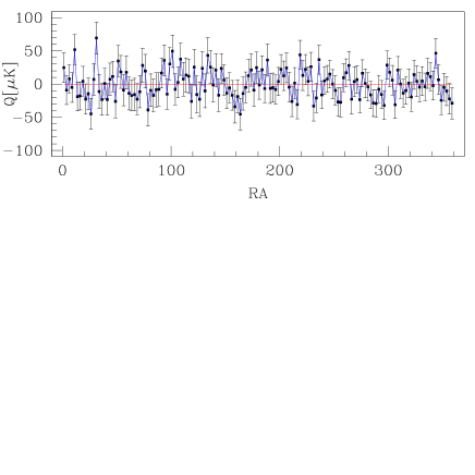
FIG. 7.: The deconvolved PIQUE data consists of the Stokes $Q$-parameter as a function of position along a $1^{\circ}$ radius circle around the North Celestial Pole. One quarter of the modes are projected out as described in the text.

$${\bf A}=\left(\begin{tabular}[]{cccc}1&1&0&0\\ 0&1&1&0\\ 0&0&1&1\\ 1&0&0&1\end{tabular}\right)~{}{\rm and}\quad{\bf x}=\left(\begin{tabular}[]{c}$Q_{1}$\\ $Q_{37}$\\ $Q_{73}$\\ $Q_{109}$\end{tabular}\right).$$ (5)

The matrix ${\bf A}$ is singular, with a vanishing eigenvalue corresponding to the vector $(1,-1,1,-1)$. Our deconvolution therefore sets this particular mode to zero, and encodes our lack of information about its value as near-infinite noise for this mode in the map noise covariance matrix. Since there are a total of 36 such pixel quadruplets, our deconvolved data set, which is plotted in Figure 7, thus has 36 such unmeasured modes.

Because PIQUE was insensitive to the unpolarized CMB component, we cross-correlated the $Q$-data from PIQUE with $T$-data from the SK map [23], deconvolved and pixelized as described in [24]. To take advantage of cross-polarization information from spatially separated pixels, we used SK pixels not merely from the PIQUE circle, but from a filled disk of radius $3^{\circ}$ around the NCP, a total of 288 $0.31^{\circ}\times 0.31^{\circ}$ pixels. We found that further increasing the size of the SK disk did not significantly tighten our constraints. Our final data vector combines the PIQUE $Q$-data and the SK $T$-data and thus contains $144+288=432$ pixels.

B Method

We compute the six power spectra describe in Section II A using quadratic estimator method as described in [7], computing fiducial power spectra with the CMBfast software [25] using cosmological parameters from the concordance model from [21]. We also perform a likelihood analysis as described below.

A key challenge is separating the six power spectra ($T,E,B,X,Y,Z$). A generic quadratic band power estimator (a quadratic combination of $T$, $Q$ and $U$ pixels) will probe a weighted average of all six power spectra, so measurements of the six can in principle be afflicted by as many as $\left({6\atop 2}\right)=15$ types of unwanted “leakage” whereby a measurement of one power spectrum picks up contributions from another. In [7] it was argued that susceptibility to systematic errors could be reduced by chosing the “priors” that determine the quadratic estimator method to have vanishing cross-polarizations, $X=Y=Z=0$, and it was shown that this simplification came at the price of a very small (percent level) increase in error bars. In Appendix A, we show that this choice has an important added benefit: exploiting a parity symmetry, it eliminates 14 out of the 15 leakeges, with only the much discussed [7, 10, 12, 13, 14, 15] $E-B$ leakage remaining. Note that whereas parity-conservation in the laws of physics predicts $Y=Z=0$, the proof given in Appendix A is purely geometric in nature, and holds even if parity-violating physics, foregrounds, etc., produce non-vanishing $Y$ and $Z$.

This result is useful in all but eliminating the leakage headache, which would otherwise complicate both calculation and interpretation. It also has important implications for other approaches, notably the currently popular maximum-likelihood (ML) method as implemented by the MADCAP software [27] and applied to Maxima, BOOMERanG, DASI and other experiments: generalizing it to polarization in the obvious way will produce the exactly the sort of leakage that our method eliminates. However, this problem can be eliminated as described below.

The quadratic estimator (QE) method is closely related to the ML method: the latter is simply the quadratic estimator method with ${\bf B}={\bf F}^{-1}$ in equation (10), iterated so that the fiducial (“prior”) power spectrum equals the measured one [28]. For a detailed comparison between these two methods, see section IV.B. in [7]. The ML method has the advantage of not requiring any prior to be assumed. The QE method has the advantage of being more accurate for constraining cosmological models — since it is quadratic rather than highly non-linear, the statistical properties the measured band power vector ${\bf q}$ can be computed analytically rather than approximated, which allows the likelihood function to be computed directly from ${\bf q}$ (as opposed to ${\bf x}$), in terms of generalized $\chi^{2}$-distributions [29].

Both methods are unbiased, but they may differ as regards error bars. The QE method can produce inaccurate error bars if the prior is inconsistent with the actual measurement. The ML method Fisher matrix can produce inaccurate error bar estimates if the measured power spectra have substantial scatter due to noise or sample variance, in which case they are unlikely to describe the smoother true spectra. A good compromise is therefore to iterate the QE method once and choose the second prior to be a rather smooth model consistent with the original measurement. The lesson to take away from Appendix A is that if the ML method is used, one should reset $X=Y=Z=0$ before each step in the iteration, thereby eliminating all leakage except between $E$ and $B$.

Table 1 – Polarization power spectrum^(a)

$\delta{\rm T}^{2}\pm\sigma^{2}\>[\mu K^{2}]$ $\Delta\l\pm\sigma_{\l}$ $\delta{\rm T}\>[\mu K]^{(b)}$ $T$ 2183 $\pm$905 151.3$\pm$ 85.8 46.7${}^{+9}_{-11}$ $E$ -2.4$\pm$ 17.4 153.4$\pm$ 87.6 $<$ 3.9 (5.7) $B$ -8.1$\pm$ 16.0 141.6$\pm$ 73.7 $<$ 2.8 (4.9) $X$ -145.5$\pm$222.2 137.4$\pm$ 69.4 $<$ 8.6(17.3) $Y$ -7.9$\pm$206.2 151.3$\pm$ 82.5 $<$14.1(20.1)

^(a)Results from combined PIQUE and SK data;
^(b)Values in parentheses are 2-$\sigma$ upper limits.

C Results

Table 1 shows the result of our band-power estimation. Here we use 50 multipole bands of width $\Delta\l=20$ for each of the six polarization types $(T,E,B,X,Y,Z)$, thereby going out to $\l=1000$, and average the measurements together into a single number for each polarization type to reduce noise. We eliminate sensitivity to offsets by projecting out the mean (monopole) from the $T$ and $Q$ maps separately. The values shown in parentheses in the most right column of Table 1 are 2-$\sigma$ upper limits (those are also the values that we present here as our upper limits).

The detection of unpolarized power is seen to be consistent with that published for the full SK map [6]. The table shows that we detect no polarization or cross-polarization of any type, obtaining upper limits, just as the concordance model predicts. No results of $Z$ are reported since PIQUE provides only $Q$ data (note that $Q$ and $U$ are needed to isolate $Z$-polarization — we will include $Z$ in in Section IV).

The window functions reveal substantial leakage between $E$ and $B$, so the limits effectively constrain the average of these two spectra rather than both separately. For this reason, and to recast our constraints in terms of the $TE$ correlation coefficient $r_{\ell}$, we complement our band-power analysis with a likelihood analysis where we assume $B=0$. Specifically, we set $B=Y=Z=0$ and take each of the remaining power spectra $(T,E,X)$ to be constant out to $\l=1000$.

We first perform a simple 1-dimensional likelihood analysis for the parameter $E$ using the PIQUE data alone (discarding the SK information), obtaining the likelihood function (bottom solid line in right panel of Figure 8) in good agreement with that published by the PIQUE team [5]. They find 95% of the area for $E<10\mu$K — our likelihood curve drops by a factor $e^{-2}$ at a slightly lower value $E\approx 7\mu$K as expected, since the likelihood curve is asymmetric and hence highly non-Gaussian. This non-Gaussianity also means that the precise confidence levels of the upper limits in Table 1 should be taken with a grain of salt. The $B$-limit is rather low because noise fluctuations give a negative best estimate (recall that what is measured is the sky power minus the expected noise power, which can be negative), and this preference for negative $B$ pulls down the $E$ estimate too since the strong leakage implies that it is really measuring a weighted average of $E$ and $B$.

We then compute the likelihood function including both PIQUE and SK data in the 3-dimensional space spanned by $(T,E,r_{\ell})$ and compute constraints on individual parameters or pairs by marginalizing as in [21]. Figure 8 shows that this produces a $T$-measurement $T\approx 50\mu$K, consistent with that for the full SK map [6] (left panel). Figure 9 shows our constraints in the $(E,r_{\ell})$-plane after marginalizing over $T$. The “C” shape of the contours in here are not generic: we performed a series of Monte Carlo simulations, and some produced “backward C” shapes instead, others “S”-like shapes. This figure also shows that our constraints on the cross-polarization are weaker than the Schwarz inequality $r_{\ell}\leq 1$, so in this

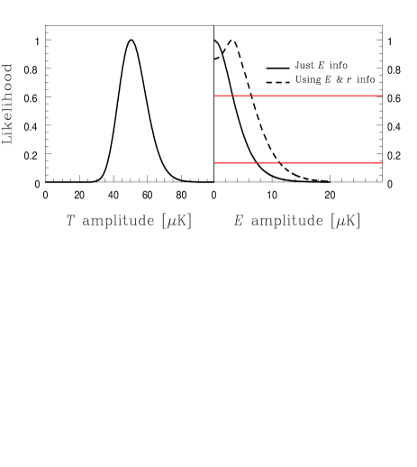
FIG. 8.: Likelihood results using PIQUE $Q$-information alone (right panel, solid line) and using both PIQUE $Q$- and SK $T$-information and marginalizing (remaining two curves). From top to bottom, the two horizontal red lines correspond to 68% and 95% of C.L., respectively.

FIG. 9.: Joint constraints on $E$ polarization and $r_{\ell}$ after marginalizing over $T$. From left to right, the contours show that the likelihood function has dropped to $e^{-1.1}$, $e^{-3.0}$ and $e^{-4.6}$ times its maximum value, which would correspond to 68%, 95% and 99% limits if the likelihood were Gaussian. For comparison, the concordance model predicts ($E,r_{\ell}$)=(0.82,-0.65) at $\l$=137, the center of our window function for $X$ (see Table 1).

sense the data has taught us nothing new. This funny situation is unique to measuring correlations, since any measurement of say $T$ or $E$, however noisy, will always rule out some class of theoretically allowed models. However, it is important to point out that this failure to beat the Schwartz inequality does not mean that an experiment is far from detecting polarization: as we saw in Section II C, the actual correlation coefficient can be of order unity, so the step from overcoming the Schwartz bound to detecting an $X$-signal may in fact be quite small. Figure 10 summarizes all polarization limits published to date, and indicates that the detection of cross-polarization may indeed be just around the corner.

Cross-polarization information could, in principle, reduce error bars on $E$ as well. As an extreme example, if we had measured that $r_{\ell}\approx 1$ on the angular scales probed by PIQUE, with tiny error bars, then we would know the exact spatial template of the $E$-map from the $T$-map and could therefore fit for its amplitude quite accurately. The effect of adding cross-polarization information on the PIQUE $E$-limits is shown in Figure 8 (dashed line in right panel). In this case, we had no meaningful constraints on $r_{\ell}$, so it is not surprising that this approach does not help us: we see that adding the unpolarized temperature simply weakens the upper limit slightly courtesy of noise fluctuations.

Since $r_{\l}$ is expected to oscillate between positive and negative values, using a flat (constant) $r_{\l}$ in the likelihood analysis runs the risk of failing to detect a signal that is actually present in the data, canceling out positive and negative detections at different angular scales. This is not likely to have been a problem in our case, since $r_{\l}$ is uniformly negative in our sensitivity range $\l=137\pm 69$ for the concordance model, but for future experiments with higher signal-to-noise, it will be important to parametrize $r_{\l}$ in a more physical way - either with separate bandpowers in multiple bands or directly in terms of cosmological parameters.

D Future prospects

What improvements in data would enhance the scientific potential of an experiment like PIQUE the most? Reducing the noise level in the polarization measurements would obviously improve the limits on $E$, $B$ and $r_{\l}$. We find that substantial reductions would be needed to make a qualitative difference – a simulation merely doubling the amount of data, adding $U$-polarization, did not produce an $r_{\l}$-detection or beat the Schwarz inequality. Figure 11 shows which sort of sensitivity improvements are needed for a marginal detection in the $E$–$r_{\l}$ plane using the same number and position of pixels as for PIQUE. The Schwarz bound inequality is seen to be beaten by a substantial margin on the high side. This illustrates the potential value of experimental groups coordinating to observe the same sky regions. Increased sky coverage and a more two-dimensional geometry clearly helps, and we explore such an example in the next section.

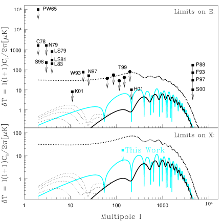
FIG. 10.: Summary of upper limits on polarization so far. From top to bottom, the three curves show the concordance model predictions for $C_{\l}^{T}$, $C_{\l}^{E}$ and $C_{\l}^{X}$, respectively. Four reionization models with $\tau$=0.1, 0.2, 0.3 and 0.4 are also plotted (left thin lines from bottom to top). The limits are: PW65[32], C78[33], N79[34], LS79[35], LS81[36], S98[37], L83[38], W93[39], N97[6], T99 hexagons[40], P88[41], F93[42], P97[43], S00[44], H01[5] and K01[11] (all in upper panel) and our new upper limit on $X$ (lower panel).

FIG. 11.: $E$–$r_{\ell}$ likelihood for the case of lower noise (50 $\mu$K per SK pixel, 5 $\mu$K per PIQUE pixel), showing that this sensitivity level can give interesting constraints on $r_{\ell}$. The data used here is a Monte Carlo simulation with ($E,r_{\ell}$)=(0.82,-0.65), which is what the concordance model predicts at $\l$=137, the center of our window function for $X$ (see Table 1).

FIG. 12.: Constraints in the $E$-$r_{\ell}$ plane from a simulation of the ${\rm BOOMERanG}$ experiment. From outside to inside, the likelihood contours are same as in Figure 9. A fiducial model with $C_{\l}^{E}=1\mu$K and $C_{\l}^{X}$=0 was used in this calculation.

IV Case study II: ${\rm BOOMERanG}$ data

We begin case study II by extending the results presented in [7]. In this section we quantify the ability of ${\rm BOOMERanG}$ to separate the $Y$ and $Z$ correlations using $(T,Q,U)$ maps.

We pixelize our sky patch using the equal-area icosahedron method [30] at resolution levels 35, corresponding to 361 ${\rm BOOMERanG}$ pixels. We apply the quadratic estimator described in [7] just as we did for PIQUE, with the fiducial power spectra $C_{\l}^{T}$ computed using CMBfast software [25] using cosmological parameters from the concordance model from [21]. In our fiducial model we set $C_{\l}^{E}=1\mu$K² and $C_{\l}^{B}=C_{\l}^{X}=C_{\l}^{Y}=C_{\l}^{Z}=0$, and eliminate sensitivity by offsets by projecting out the mean (monopole) for $T$, $Q$ and $U$ maps separately.

Figure 12 shows how important the unpolarized counterpart is when constraining the polarized power spectrum: high signal–to–noise temperature data is seen to substantially improve how well $E$ can be constrained. The $1\mu$K $E$ signal used in our case study is detected at high significance when using polarization data alone. Although adding $T$-information is obviously necessary to constrain $r_{\l}$, we found that it helped only marginally for constraining $E$: we repeated our likelihood analysis using $T$, $Q$ and $U$ data jointly, marginalizing over $T$ and $r_{\l}$, and obtained essentially unchanged error bars.

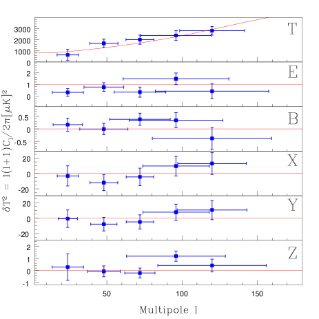
FIG. 13.: ${\rm BOOMERanG}$ power spectrum $T,E,B,X,Y$ and $Z$. The power spectrum was calculated for 5 bands of size $\Delta\l$=24, $C_{\l}^{T}$ was computed using CMBfast software, and we assumed $C_{\l}^{E}$=1 and $C_{\l}^{B}=C_{\l}^{X}=C_{\l}^{Y}=C_{\l}^{Z}=0$ when running our Monte Carlos.

Finally, Figure 13 shows that we can separate the $Y$ and $Z$ correlations if we use $(T,Q,U)$ maps jointly. We also verified numerically that there is no leakage between the $TB$ and $EB$ correlations, as proved in Section VI. Note that the results in this section underestimates the true power of Boomerang 2002 by only using enough pixels to probe the power out to $\l\sim 120$, the key intention being simply to demonstrate that the both experimental sensitivity and our analysis method is adequate. When the real data is available, a more computer intensive analysis with or order $10^{4}$ pixels will be worthwhile.

V CONCLUSIONS

We have presented the first attempt at measuring the CMB cross-polarization, using the PIQUE and SK data sets. We obtain upper limits of $TE\equiv X<$ 8.6 $\mu$K (95% CL) and $TB\equiv Y<$ 14.1 $\mu$K (95% CL). Limits for $E$ are in concordance with the values presented in [5], and are much higher than the expected NCP foreground levels [45, 5]. We also discuss theoretical and practical issues relevant to measuring cross-polarization and illustrate them with simulations of the upcoming ${\rm BOOMERanG}$ 2002 experiment: we find that substantial improvements on measuring the polarized power spectra would be possible if the noise could be lowered in the unpolarized map used for the cross-correlation. Among other things, we show that the well-known problem of $EB$ leakage, which complicates measurements of $E$ and $B$ power, vanishes when measuring the three cross-polarization power spectra ($TE$, $TB$ and $EB$).

VI Appendix

In this appendix, we prove the no-leakage theorem described in the text. Specifically, we show that that our quadratic estimator method gives no leakage between any of the 15 power spectrum pairs except E/B.

We follow the notation of [7] throughout. We let ${\bf x}$ denote the vector that contains the measured temperature and Stokes parameters at each pixel and consider quadratic estimators of the different power spectra,

$$q_{i}\equiv{\bf x}^{t}{\bf Q}_{i}{\bf x}=\hbox{tr}\>[{\bf Q}_{i}{\bf x}{\bf x}^{t}],$$ (6)

where $i$ labels at the same time both the polarization type $P$ ($T,E,B,X,Y$ and $Z$) and the multipole $\l$ to be measured. $q_{i}$ probes a weighted average of the power spectra,

$$\langle q_{i}\rangle = \hbox{tr}\>[{\bf Q}_{i}{\bf C}]$$ (7)

$$= b+\sum_{P^{\prime}=1}^{6}\sum_{\l^{\prime}=2}^{\ell_{\rm max}}W^{\l P}_{\l^{\prime}P^{\prime}}C_{\l^{\prime}}^{P^{\prime}},$$ (8)

where $b\equiv\hbox{tr}\>[{\bf Q}_{i}{\bf\Sigma}]$ is the contribution from experimental noise, ${\bf\Sigma}$ is the noise covariance matrix, $\SS$ is the covariance matrix due to the cosmological signal, and ${\bf C}={\bf\Sigma}+\SS$ is the total covariance matrix. In equation (7) we introduced generalized window functions,

$$W^{\l P}_{\l^{\prime}P^{\prime}}\equiv\hbox{tr}\>[{\bf Q}_{i}{\bf P}_{i^{\prime}}],$$ (9)

where ${\bf P}=\partial{\bf C}/\partial C_{l}^{P}$. For a fixed $(P,\l)$, they show the expected contributions to the band power estimate $q_{i}$ not only from different $\l$-values, but also from different polarization types. For instance, an estimate of $E$-polarization may inadvertently pick up a contribution from $B$-polarization as well, since it is difficult to separate the two with only partial sky coverage [7, 10, 12, 13, 14, 15]. Such leakage between different polarization types is clearly undesirable since it complicates interpretation of the measurements. The aim of the appendix is to show that for our particular choice of estimator ${\bf Q}_{i}$, most elements of the window functions $W^{\l P}_{\l^{\prime}P^{\prime}}$ vanish, and that there is indeed no other leakage than between any E and B — not, say, between X and Y or between E and Z.

In [7] it was shown that the quadratic estimator defined by

$${\bf Q}_{i}={1\over 2}{\cal N}_{i}\sum_{j}B_{ij}{\bf C}^{-1}{\bf P}_{j}{\bf C}^{-1},$$ (10)

distills all the cosmological information from ${\bf x}$ into the (normally much shorter) vector ${\bf q}$ if ${\bf C}$ is the true covariance matrix. Moreover, if ${\bf C}$ is a reasonable estimate of the true covariance matrix, then the data compression step of going from ${\bf x}$ to ${\bf q}$ destroys information only to second order. In equation (10), ${\bf B}$ is an arbitrary invertible matrix and the normalization constants ${\cal N}_{i}$ are chosen so that all window functions sum to unity. This means that we can interpret $q_{i}$ as measuring a weighted average of our unknown parameters, the window giving the weights.

For our estimates we constructed the covariance matrix appearing in equation (10) setting $C_{l}^{X}=C_{l}^{Y}=C_{l}^{Z}=0$ and $C_{l}^{E}=C_{l}^{B}$. As explained in detail in [7], the choice $C_{l}^{X}=C_{l}^{Y}=0$ was made because it makes the estimates of the temperature power spectra only depend on quadratic combinations involving two measured temperatures, the estimates of $X$ and $Y$ only depend on quadratic combinations involving one Stokes parameter and one temperature and the estimate of the $E$, $B$ and $Z$ spectra only depend on products of two Stokes parameters (otherwise additional non-intuitive terms get included, say temperature autocorrelations when measuring $E$, increasing susceptibility to systematic errors). These facts immediately imply that the only mixed windows that could potentially be non-zero are $W^{\l E}_{\l^{\prime}B},\ W^{\l X}_{\l^{\prime}Y},\ W^{\l E}_{\l^{\prime}Z},\ W^{\l B}_{\l^{\prime}Z}$, i.e., that of the $\left({6\atop 2}\right)=15$ types of potential leakage, only EB, XY, EZ and BZ leakage is possible. What we will show in this appendix using an argument based on the parity of the different fields is that only $W^{\l E}_{\l^{\prime}B}$ is non-zero for our choice of ${\bf C}$.

We consider a parity transformation such that the coordinate ${\bf r}^{\prime}=-{\bf r}$, where primes indicate the coordinates after the transformation. We define the operator ${\bf\Pi}$ to be the one that transforms the vector of temperatures and Stokes parameters ${\bf x}$ under the parity transformation, ${\bf x}^{\prime}={\bf\Pi}{\bf x}$. It satisfies ${\bf\Pi}^{2}={\bf I}$, the identity. For example, if the Stokes parameters at each point on the sky were defined with respect to the spherical coordinate system, then ${\bf\Pi}$ transforms them as $Q^{\prime}=Q$ and $U^{\prime}=-U$. Under a parity transformation, we also have $T^{\prime}=T$, $E^{\prime}=E$ and $B^{\prime}=-B$.

To understand how the matrices ${\bf C}$ and ${\bf P}$ behave under parity, we need to understand their structure. Let us consider an arbitrary pair of points labeled $A$ and $B$. The matrices are most easily described when the Stokes parameters are measured with respect to the natural frame, that is when $Q$ is defined as the differences in intensity in the directions parallel and perpendicular with respect to the great circle that joins $A$ and $B$. In that case the structure of the covariance matrix is,

$$\langle T_{A}T_{B}\rangle = \sum_{l}f_{1}^{\l}C_{\l}^{T}$$ (11)

$$\langle Q_{A}Q_{B}\rangle = \sum_{l}f_{2}^{\l}C_{\l}^{E}+f_{3}^{\l}C_{\l}^{E}$$ (12)

$$\langle U_{A}U_{B}\rangle = \sum_{l}f_{2}^{\l}C_{\l}^{B}+f_{3}^{\l}C_{\l}^{B}$$ (13)

$$\langle T_{A}Q_{B}\rangle = \sum_{l}f_{4}^{\l}C_{\l}^{X}$$ (14)

$$\langle T_{A}U_{B}\rangle = \sum_{l}f_{4}^{\l}C_{\l}^{Y}$$ (15)

$$\langle U_{A}Q_{B}\rangle = \sum_{l}(f_{2}^{\l}-f_{3}^{\l})C_{\l}^{Z}$$ (16)

where the coefficients $f^{\l}_{i}$ are known functions of the angular separation between $A$ and $B$. From the above expressions we can calculate what the different ${\bf P}$-matrices are in this frame. The matrix ${\bf P}_{T}$ has non-zero entries only for the terms involving $T_{A}$ and $T_{B}$, $P_{E}$ and $P_{B}$ only terms involving $Q_{A}$ $Q_{B}$ and $U_{A}$ $U_{B}$, ${\bf P}_{X}$ only for those involving $Q_{A}$ $T_{B}$ and $Q_{B}$ $T_{A}$, ${\bf P}_{Y}$ only for those involving $U_{A}$ $T_{B}$ and $U_{B}$ $T_{A}$ and ${\bf P}_{Z}$ only for those involving $Q_{A}$ $U_{B}$ and $Q_{B}$ $U_{A}$. Moreover if when constructing ${\bf C}$ we took $C_{\l}^{X}$ and $C_{\l}^{Y}$ to be zero, ${\bf C}$ is block diagonal, with no terms that mix $T$ and $Q$ or $T$ and $U$. It is clear then why our estimators of $X$ and $Y$ only contain $TQ$ and $TU$ terms.

Under a parity transformation in this coordinate system, the Stokes parameters transform as $T^{\prime}=T$ , $Q^{\prime}=Q$ and $U^{\prime}=-U$. Under parity in (11), the last two equations change sign while the others remain the same. Thus if ${\bf C}$ was constructed assuming that all the cross spectra were zero, which implies that the last three expectation values in equation (11) are zero, then ${\bf\Pi}{\bf C}{\bf\Pi}={\bf C}$ which implies that ${\bf\Pi}{\bf C}^{-1}{\bf\Pi}={\bf C}^{-1}$. Furthermore because only the last two equations in (11) change sign, the ${\bf P}$ matrices satisfy ${\bf\Pi}{\bf P}_{T}{\bf\Pi}={\bf P}_{T}$, ${\bf\Pi}{\bf P}_{E}{\bf\Pi}={\bf P}_{E}$, ${\bf\Pi}{\bf P}_{B}{\bf\Pi}={\bf P}_{B}$, ${\bf\Pi}{\bf P}_{X}{\bf\Pi}={\bf P}_{X}$, ${\bf\Pi}{\bf P}_{Y}{\bf\Pi}=-{\bf P}_{Y}$ and ${\bf\Pi}{\bf P}_{Z}{\bf\Pi}=-{\bf P}_{Z}$. In other words, the $Y$ and $Z$ spectra are odd under parity while the $T$, $E$ and $X$ ones are even.

We now have all the necessary ingredients to show that any cross window function that involves spectra with different parity will be zero. These window functions will be given by the values of $\hbox{tr}\>[{\bf C}^{-1}{\bf P}_{i}{\bf C}^{-1}{\bf P}_{i^{\prime}}]$. If the two ${\bf P}$-matrices have different parities, we have

$$\hbox{tr}\>[{\bf C}^{-1}{\bf\Pi}{\bf P}_{i}{\bf\Pi}{\bf C}^{-1}{\bf\Pi}{\bf P}_{i^{\prime}}{\bf\Pi}]=-\hbox{tr}\>[{\bf C}^{-1}{\bf P}_{i}{\bf C}^{-1}{\bf P}_{i^{\prime}}].$$ (17)

Using the fact that ${\bf C}^{-1}$ commutes with ${\bf\Pi}$ and the cyclic property of the trace, we get

$$\hbox{tr}\>[{\bf C}^{-1}{\bf P}_{i}{\bf C}^{-1}{\bf P}_{i^{\prime}}]=-\hbox{tr}\>[{\bf C}^{-1}{\bf P}_{i}{\bf C}^{-1}{\bf P}_{i^{\prime}}].$$ (18)

Thus if ${\bf P}_{i}$ and ${\bf P}_{i^{\prime}}$ have different parities, the trace will be zero. With our choice of ${\bf C}$, the window functions mixing spectra with different parities are identically zero. This means that there is no leakage between X and Y, between E and Z or between B and Z, so the only non-zero mixed window function is $W^{\l E}_{\l^{\prime}B}$. In other words, out of the 15 potential leakages, our method eliminates all except that between E and B.

Support for this work was provided by NASA grants NAG5-9194 and NAG5-11099, NSF grant AST00-71213, and two awards from the David and Lucile Packard Foundation.

REFERENCES

- [1] M. Zaldarriaga and D. Harari, Phys.Rev. D 52, 2 (1995).
- [2] W. Hu and M. White, New Astron. 2, 323 (1997).
- [3] M. Zaldarriaga, D. Spergel and U. Seljak, ApJ 488, 1 (1997).
- [4] M. Tegmark, D. J. Einsenstein, W. Hu , and A. de Oliveira-Costa, ApJ 530, 133 (2000).
- [5] M. Hedman et al., ApJL 548, L111 (2001).
- [6] C. B. Netterfield et al., ApJ 474, 47 (1997).
- [7] M. Tegmark and A. de Oliveira-Costa, Phys.Rev. D 64, 063001 (2001).
- [8] A. Kamionkowski, A. Kosowsky, and A. Stebbins, Phys.Rev. D 55, 7368 (1997).
- [9] M. Zaldarriaga and U. Seljak, Phys.Rev. D 55, 1830 (1997).
- [10] M. Zaldarriaga, ApJ 503, 1 (1998).
- [11] B. Keating et al., ApJ 560, 1 (2001).
- [12] A. H. Jaffe, M. Kamionkowski, and L. Wang, Phys.Rev. D 61, 083501 (2000).
- [13] M. Zaldarriaga, astro-ph/0106174 (2001).
- [14] A. Lewis, A. Challinor, and N. Turok, Phys.Rev. D 65, 023505 (2002).
- [15] E. F. Bunn, astro-ph/0108209 (2001).
- [16] M. Kamionkowski, and A. Kosowsky, Ann.Rev. Nucl. Part. Sci. 49, 77 (1999).
- [17] X. Chen, and M. Kamionkowski, Phys.Rev. D 60, 104036 (1999).
- [18] M. Kamionkowski , and A. H. Jaffe, Int.J.Mod.Phys. A 16, 116 (2001).
- [19] W. Hu , and M. White, Phys.Rev. D 56, 596 (1997).
- [20] M. Zaldarriaga, and U. Seljak, Phys.Rev. D 580, 3003 (1998).
- [21] X. Wang, M. Tegmark, and M. Zaldarriaga, astro-ph/0105091 (2001).
- [22] G. Efstathiou et al., astro-ph/0109152 (2001).
- [23] M. Tegmark et al., ApJL 474, 77 (1997).
- [24] Y. Xu et al., astro-ph/0010552 (2001).
- [25] U. Seljak, and M. Zaldarriaga, ApJ 469, 437 (1996).
- [26] M. Zaldarriaga, Phys.Rev. D 55, 1822 (1997).
- [27] J. Borrill, astro-ph/9911389 (1999).
- [28] J. R. Bond, A. H. Jaffe, and L. E. Knox, ApJ 533, 19 (2000).
- [29] B. D. Wandelt, astro-ph/0012416 (2000).
- [30] M. Tegmark, ApJL 470, L81 (1996).
- [31] K. M. Gorski, B. D. Wandelt, F. K. Hansen, E. Hivon, and A. J. Banday, astro-ph/9905275 (1999).
- [32] A. A. Penzias, and R. W. Wilson, ApJ 142, 419 (1965).
- [33] N. Caderni, Phys.Rev. D 17, 1908 (1978).
- [34] G. Nanos, ApJ 232, 341 (1979).
- [35] P. M. Lubin, and G. F. Smoot, Phys.Rev. Lett. 42(2), 129 (1979).
- [36] P. M. Lubin, and G. F. Smoot, ApJ 245, 1 (1981).
- [37] G. Sironi, G. Boella, G. Bonelli, L. Brunetti, F. Cavaliere, M. Fervasi, G. Giardino, and A. Passerini, New (1998).Astronomy;3;1
- [38] P. M. LubinP. Melese, and G. F. Smoot, ApJ;273;51 (1983).
- [39] E. J. Wollack, N. C. Jarosik, C. B. Netterfield, L. A. Page, and D. Wilkinson, ApJ;419;49 (1993).
- [40] E. Torbet, M. J. Devlin, W. B. Dorwart nn Herbig T, A. D. Miller, M. R. Nolta, L. A. Page, J. Puchalla, and H. Tran T, ApJ 521, 79 (1999).
- [41] R. B. Partridge, J. Nawakowski, and H. M. Martin, Nature 311, 146 (1988).
- [42] E. B. Fomalont, R. B. Partridge, J. D. Lowenthal, and R. A. Windhorst, ApJ 404, 8 (1993).
- [43] R. B. Partridge, E. A. Richards, E. B. Fomalont, K. I. Kellerman, and R. A. Windhorst, ApJ 483, 38 (1997).
- [44] R. Subrahmanyan, M. J. Kesteven, R. D. Ekers, M. Sinclair, and J. Silk, MNRAS 315, 808 (2000).
- [45] A. de Oliveira-Costa et al., ApJL 482, L17 (1997).
- [46] S. L. Wheelock et al., IRAS (1994).Sky Survey Atlas: Explanatory Supplement (Pasadena: JPL 91-11)
- [47] W. N. Brouw, and T. A. T Spoelstra, A&AS 26, 129 (1976).
- [48] C. G. T Haslamet al., A&AS 47, 1 (1982).