Detailed Spectroscopic Analysis of SN 1987A: The Distance to the LMC using the SEAM method

Abstract

Supernova 1987A remains the most well-studied supernova to date. Observations produced excellent broad-band photometric and spectroscopic coverage over a wide wavelength range at all epochs. We model the observed spectra from Day 1 to Day 81 using a hydrodynamical model. We show that good agreement can be obtained at times up to about 60 days, if we allow for extended nickel mixing. Later than about 60 days the observed Balmer lines become stronger than our models can reproduce. We show that this is likely due to a more complicated distribution of gamma-rays than we allow for in our spherically symmetric calculations. We present synthetic light curves in $UBVRIJHK$ and a synthetic bolometric light curve. Using this broad baseline of detailed spectroscopic models we find a distance modulus of $\mu=18.5\pm 0.2$ using the SEAM method of determining distances to supernovae. We find that the explosion time agrees with that of the neutrino burst and is constrained at 68% confidence to within $\pm 0.9$ days. We argue that the weak Balmer lines of our detailed model calculations casts doubt on the accuracy of the purely photometric EPM method. We also suggest that Type IIP supernovae will be most useful as distance indicators at early times due to a variety of effects.

1 Introduction

Observations of SN 1987A produced extensive broad-band photometry and excellent spectroscopic coverage. This motivated the development of models to predict its spectral and photometric evolution. In our analysis here we make use of the optical data obtained at the Cerro Tololo Inter-American Observatory (CTIO) (Phillips et al., 1988) and the extensive International Ultraviolet Explorer (IUE) data which were obtained, re-reduced and analyzed by Pun et al. (1995).

While SN 1987A led to the growth of observational data, so too did it lead to an improvement in theoretical models. Höflich (1991) modeled the early phase of SN 1987A, using a pure hydrogen atmosphere and accounting for Non-Local Thermodynamic Equilibrium (NLTE). Eastman & Kirshner (1989) modeled the first ten days of the SN 1987A explosion. H I and He I were modeled in NLTE, while metal lines were treated as pure scattering LTE lines. The pure H/He non-LTE model of Takeda (1991) resulted in weak Balmer lines, as did a model by Hauschildt & Ensman (1994), which used an earlier version of PHOENIX with H I, He I, Mg II, and Ca II in NLTE and metal line blanketing in LTE. These two groups suggested that differences between the theoretical and actual density distributions might be responsible for the discrepancy between the synthetic and observed Balmer lines.

We use the light curve model of Blinnikov and collaborators calculated using the STELLA software package (Blinnikov et al., 1998; Blinnikov, 1999; Blinnikov et al., 2000). This model simulates the light curve for up to six months after the explosion, and includes allowance for time-dependent, multi-group radiation hydrodynamics, monochromatic scattering effects, and the effects of spectral lines on the opacity (Blinnikov et al., 2000). The light curve model was based on the stellar evolution models of Saio, Nomoto, & Kato (1988), Saio, Kato, & Nomoto (1988), and Nomoto & Hashimoto (1988). The procedure for synthesizing SN 1987A spectra from Blinnikov et al.’s model and the results are described in § 2. In § 3 we compare our synthetic spectra to observations. § 4 compares our synthetic light curves with observations and we derive a distance to SN 1987A. In a final section we discuss the implications of our results for the use of SNe II as distance indicators.

2 Models

2.1 PHOENIX

PHOENIX is a general radiation transfer code that computes temperature, opacity, and level populations for each of typically 50–100 radial zones in a moving stellar envelope. PHOENIX solves the full NLTE rate equations and calculates level populations for a multitude of different atomic species in LTE or NLTE (Hauschildt & Baron, 1999; Short et al., 1999). For this study, the following species were calculated in NLTE: H I(30/435), He I(19/37), He II(10/45), O I(36/66), Ne I(26/37), Na I(53/142), Mg II(72/340), Si II(93/436), S II(84/444), Ca II(87/455), Fe I(494/6903), Fe II(617/13675), and Fe III(566/9721), where e.g. H I(30/435) indicates that our model atom for H I contains 30 levels and 435 permitted transitions treated in full NLTE.

The Blinnikov et al. light curve model consists of an ejecta envelope divided into 300 zones, with compositions defined for each layer (Blinnikov, 1999; Blinnikov et al., 2000). The outer layers of this model were re-zoned onto the 75–100 zone grid that is used by PHOENIX, preserving the compositions in velocity-space. The radius, density, and compositions were taken from the Blinnikov et al. model and interpolated onto the new grid. The inner boundary condition was taken to be diffusive, which is well justified in these calculations. The total bolometric luminosity provides the outer boundary condition and we generally take the value from the results of Blinnikov et al. (2000). However since the bolometric luminosity is a parameter, we study the effects of varying it to improve the fit to the observed spectra. After about 18 days from the explosion we find that the values predicted by the light curve calculations need to be adjusted in order for the synthetic spectra to match the observations. We adjust the bolometric luminosity to find the best fit to the observed spectra, we do not attempt to use the photometry as a fitting parameter in any way. All synthetic photometry is an output of our calculations once we have calculated the synthetic spectrum. The temperature is determined self-consistently from the generalized condition of radiative equilibrium. We use the initial temperature from Blinnikov et al. as our initial guess. The gamma-ray energy deposition rate, which is the energy in gamma-rays deposited in the matter in the envelope per unit mass per unit time, is calculated for each new zone. We calculate the gamma-ray deposition function using our self-consistent spherically symmetric radiative transfer code, assuming a gray opacity for gamma-rays of $0.06$ cm² g^-1 (Swartz et al., 1995; Colgate et al., 1980). Our calculational grid was chosen so as to maintain both composition and density profiles with adequate resolution.

3 Synthetic Spectra

Figures 1–3 show the spectra resulting from PHOENIX computations on days 1.36, 2.67, and 3.59, respectively, of SN 1987A. The fits between the IUE spectra and the synthetic UV spectra are very good, an indicator of the importance of NLTE effects in the supernova envelope (Baron et al., 1996b). Blinnikov et al. (2000) noted that the predicted UV flux 5–10 days after shock breakout was much greater than the actual flux when computed in LTE, but this also may have been due to not enough line blanketing in these initial calculations (E. Sorokina et al., in preparation). We included over 1 million lines in all our calculations and they are dynamically selected to be the most important lines for the conditions, thus line blanketing is well accounted for in these calculations. For days 1.36 and 2.67, the agreement between the synthetic and observed optical spectra is also reasonably good. In day 1.36 the blueshifted absorption of the Mg h+k line does not extend far enough to the blue. The observed feature extends to 43,000 km s^-1, however the hydro model only extends to 33,500 km s^-1. Since Mg h+k is a resonance line it is optically thick all the way to the surface and the blue absorption is sensitive to the outermost layers of the model. Similar results were found by Hauschildt & Ensman (1994) using a different hydro model and an earlier version of PHOENIX.

By day 3.59 a discrepancy in the strengths of the Balmer lines begins to appear in the synthetic spectra, most notably H$\alpha$, even when NLTE effects are included. Figure 4 shows the synthetic optical/near-UV spectrum for day 4.52 compared with the observations (Phillips et al., 1988; Pun et al., 1995), and here the Balmer lines are clearly much weaker in the synthetic spectrum than they are in the observed spectrum. As we showed in Mitchell et al. (2001), we can improve the fit to the Balmer lines significantly by increasing the gamma-ray deposition in the outer layers. The result is displayed in Figure 5 where we have replaced the self-consistent gamma-ray deposition function with one that would be obtained from a uniform nickel mass fraction of $\mathrm{X}_{\mathrm{Ni}}=1.0\times 10^{-3}$ in the envelope. The fit between the predicted lines and the actual lines is much better in the optical, but the UV is no longer fit as well. This shows that the true nickel deposition is more complicated and we have overestimated the nickel deposition in the very outer layers where the line-blanketed UV is formed. We have chosen a simple parameterization to enhance the gamma-ray deposition, i.e., the gamma-ray deposition follows the density of the model. It is certainly possible (and even plausible) that there exists a spherically symmetric gamma-ray deposition function that fits both the optical and the UV, however the parameter space is large and it is beyond the scope of this work to find “the” correct gamma-ray deposition for each epoch. Nevertheless our results are a strong indication for enhanced nickel mixing in SN 1987A. As noted by Mitchell et al. (2001) the enhanced nickel mixing improves both the strength of H$\alpha$ and the velocity (as can be seen by comparing Figs. 5 and 4). Utrobin & Chugai (2002) find that the velocity and strength of H$\alpha$ can be well fit by taking into account the effect time dependence of the hydrogen non-thermal excitation and ionization (the ionization freeze-out) up to about 30 days, without invoking large ⁵⁶Ni mixing.

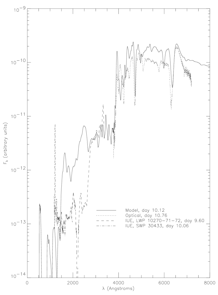
Figure 8: PHOENIX model spectrum for day 10.12, with additional nickel mixing.

Figure 6 shows the synthetic spectrum compared to the optical and IUE spectra on day 8. We have assumed uniform nickel mixing of $\mathrm{X}_{\mathrm{Ni}}=1.0\times 10^{-4}$. Comparing this to the day 4 spectrum, we can see that there is not quite enough nickel mixing to produce the Balmer lines, but the UV won’t allow for more mixing in the simple parameterization we employ. Figure 7 shows the day 10 spectrum with no additional nickel mixing and again the Balmer lines are far too weak, and only the overall color in the optical is reproduced. Figure 8 shows that nickel mixing improves the blue and the strength of the Balmer lines, however the overall fit is not better. Figure 9 shows the day 14 spectrum, with nickel mixing assumed. The overall fit is not bad in the optical, but again with the too simple deposition function the UV fit is poor. The synthetic spectrum shows a weak feature that has been identified as Ba II (see Williams, 1987; Jeffery & Branch, 1990), but since s-process enhancements have not been included in the stellar evolution model we use we don’t expect to reproduce the observed strength of this or other s-process elements. The Na I feature is far too weak in the synthetic spectrum.

Figure 10 shows the synthetic and observed spectra of day 19, where we have both assumed uniform mixing with $\mathrm{X}_{\mathrm{Ni}}=1.0\times 10^{-4}$, and we have increased the bolometric luminosity (a boundary condition for our modeling) of the model by 26% over that obtained from the light curve calculations. We find that if we simply use the bolometric luminosity of Blinnikov et al. (2000) we can not reproduce the observed spectra, but the variations we employ are well within the errors of Blinnikov et al. (2000) (see their figure 15). We have performed a series of calculations where the bolometric luminosity is varied and only present the best fits here. The best fits are obtained using the spectra only, no attempt was made to use photometric colors or any photometric data. The synthetic photometry is an output of our calculations. Except for a significant over-prediction of the flux just redward of Ca H+K, the fit is not bad. The Balmer lines are mostly too weak, but the Na D feature is significantly stronger than just 4 days earlier, even though we have increased the target luminosity of the model over that obtained from the light-curve calculation. Figure 11 shows the spectra at day 24, where again we assume constant nickel mixing and have increased the bolometric luminosity by 31%. Figure 12 shows the spectra at day 31 and the fit from the near UV to the optical is quite good. The flux is too low compared to that in the IUE SWP band. Even without additional nickel mixing the H$\alpha$ line is reasonably reproduced. Figure 13 shows the optical spectrum at day 58 and again the H$\alpha$ line is well reproduced. The structure of the Balmer lines is in fact dependent not only on the amount of nickel mixing, but also on the details of the density structure as the pseudo-photosphere recedes in mass. We have performed a series of test calculations to verify this (P. Nugent et al., in preparation). In the observations H$\beta$ is blended with an Fe II line just to the red, in the models the lines are unblended and H$\beta$ appears too strong. This may be due to the nickel mixing in the supernova, which leads to stronger blending of the iron than is present in the model.

Figure 14 shows that the LWP portion of the IUE spectrum is well-fit, however the SWP is not. Figure 15 shows the day 81 spectra with an increase in the bolometric luminosity of 17.5% over the light-curve value.

We have found that the calculated bolometric luminosity in the lightcurve models is too low at some epochs. We also find that the assumed mixing of nickel is also too small, particularly at early times. Our simple enhanced gamma-ray deposition (that the gamma-ray deposition follows the density) does not contain enough parameters to fit both the blue and red portions of the observed spectra. We note that the synthetic spectra are sensitive to the rate of gamma-ray deposition as a function of position in the ejecta. At early times almost the entire envelope is optically thick to gamma-rays and therefore we can estimate the total mass of nickel in the outer layers (Mitchell et al., 2001). At later times gamma-rays are transported from the inner layers into the outer shell, and gamma-rays produced in the outermost layers escape, therefore our simple gamma-ray deposition prescription cannot be used to infer a nickel mass fraction as a function of velocity, since gamma-ray deposition is non-local.

Even though it is likely that there exists a spherically symmetric deposition function that will better reproduce the observed spectra, it is clear that the distribution of nickel in SN 1987A is non-spherical. Chugai (1991) found evidence from the He I $\lambda 10830$ line for a “jetlike” ejection of ⁵⁶Ni. He found that he could fit the profile with $10^{-4}$ ${\mathrm{M}_{\odot}}$ of ⁵⁶Ni above 5000 km s^-1 and that it was consistent with $10^{-3}-10^{-5}$ ${\mathrm{M}_{\odot}}$ of nickel needed to fit the emission spectrum of the hydrogen lines. This is also consistent with our results. Haas et al. (1990) observed the [Fe II] 17.94 and 25.99 $\mu$m lines and found clear asymmetry extending to about 3500 km s^-1, these results were modeled by Nagataki (2000) using 2-D hydro and confirm the existence of an asymmetric distribution of nickel.

4 Synthetic Light Curves

4.1 SEAM Distance

We have developed an improved version of the “Expanding Photosphere Method” (EPM): the Spectral-fitting Expanding Atmosphere Method (SEAM). The EPM method (Baade, 1926; Branch & Patchett, 1973; Kirshner & Kwan, 1974) calculates distances to supernovae by assuming that the bolometric luminosity can be approximated as

$$L\approx\zeta^{2}4\pi R^{2}\sigma T^{4},$$

where $\zeta$ is the dilution factor (Hershkowitz et al., 1986a, b; Hershkowitz & Wagoner, 1987), and represents the fact that flux is diluted since the effective temperature differs from that of the photospheric temperature (By energy conservation, $\zeta$ can be both less than one or greater than one depending on how T is determined). In supernovae, homology is valid, except during the first instants of the explosion and hence $R=vt$. The velocity can be measured from the spectral lines, and $T$ is obtained from photometric colors. The time since explosion can be determined by demanding self-consistency among epochs or from the light curve (Eastman & Kirshner, 1989; Schmidt et al., 1992; Eastman et al., 1996; Hamuy et al., 2001; Leonard et al., 2002). EPM clearly suffers from the limitation that supernovae are not blackbodies and spectral line features affect the value of the colors determined observationally and the theoretical colors that must be determined from the Planck function to obtain a distance. It is also unclear just which spectral lines should be used to determine the velocity that is needed to ascertain the radius (Hamuy et al., 2001; Leonard et al., 2002). The other obvious limitation is that the method depends sensitively on the value of the dilution factors which are assumed to be a monotonic function of the color temperature.

The SEAM method (Baron et al., 1993, 1994, 1995a, 1995b, 1996a) retains the assumption of spherical symmetry, and homology $R=vt$, but uses detailed spectral models to calculate a synthetic spectrum. Then (modulo extinction, see below) since we know the entire spectral energy distribution, synthetic photometry can be used to calculate a distance modulus in every photometric band. No blackbody assumption is required, no dilution factors are needed, and the velocity is determined by the fit to all the spectral lines, not just some pre-selected set whose identities may not be certain. A time series constrains the time of explosion.

Here, we obtain the radius using the results of the hydrodynamical model and each of our models predicts the total emitted spectral energy distribution (SED) at a particular time. We can convolve our theoretical SED with any filter function and calculate the absolute magnitude in that band. If we denote the absolute magnitude in band $X$ as $M_{X}$ then the distance modulus in a particular band is $\mu_{X}$. For every band at every time we can calculate a value of $\mu_{X}$ by the relation

$$\mu_{X} = m_{X}-A_{X}-M_{X}$$

$$= m_{X}-(M_{X}+A_{X}),$$

where $m_{X}$ is the apparent magnitude in band $X$, and $A_{X}$ is the extinction in band $X$. We obtain $A_{X}$ by applying the reddening law of Cardelli et al. (1989) with $E(B-V)=0.16$ (Lundqvist & Fransson, 1996) and $R=3.1$ to the theoretical SED. This procedure defines the SEAM method. No assumption about the shape of the SED is made since it is determined by the fit to the observed spectrum.

The distance to the LMC is of great importance in establishing the cosmological distance ladder. The value of the Hubble constant depends crucially on the calibration of Cepheids (Tonry, 2001), which is dependent on the distance to the LMC. Recent reviews of the distance to the LMC are in Gibson (2002) and Feast (2001). We focus here specifically on the distance to SN 1987A, but note that the distance to the center of the LMC is about $\mu=0.03\pm 0.03$ nearer than to the supernova (McCall, 1993) and that a recent determination to the eclipsing binary HV 2274 gives $\mu=18.46\pm 0.06$ (Groenewegen & Salaris, 2001).

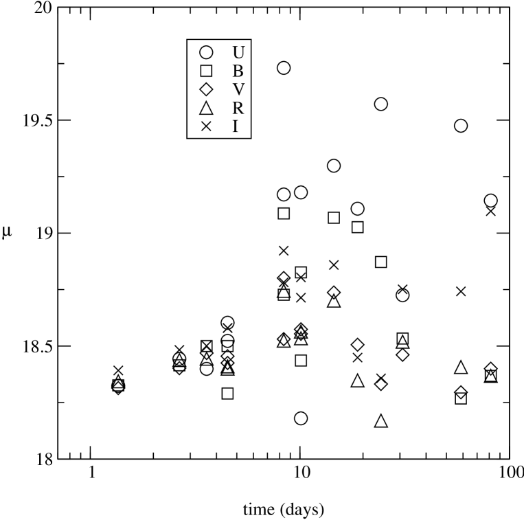
Figure 16: The distance modulus obtained from the 15 models we have calculated. The distance modulus is obtained using the photometry of Catchpole et al. (1987), Menzies et al. (1987), and Hamuy & Suntzeff (1990). The small spread at early times shows that the SEAM method is likely to be most accurate at these epochs (see text and Figure 17).

Figure 16 shows the results for the bands $UBVRI$. The observed photometry was taken from Catchpole et al. (1987) and Menzies et al. (1987) for the earliest times ($t<4$ days), and from Hamuy & Suntzeff (1990) for all other epochs. The $U$ band as expected has a lot of scatter since it is quite sensitive to the assumed nickel distribution. The mean distance is $\mu=18.6\pm 0.3$ using all the bands. The quoted error here and below is just the 1-$\sigma$ error, assuming the errors are Gaussian random errors. If we limit ourselves to $VRI$ then we obtain $\mu=18.5\pm 0.2$.

Table 1 reveals the surprising result that the large scatter is not limited to $U$ and $B$ but that the $I$ band shows more scatter than does $R$. Conventional wisdom dictates that $R$ should not be used for distance determinations because it includes H$\alpha$, however our results don’t bear this out. Hamuy et al. (2001) found that synthetic $I$ magnitudes on observed spectra had errors at the level of $\sim 0.1$ mag, which may explain, e.g, the large discrepancy in the value of $\mu_{I}$ on day 81 in Figure 16.

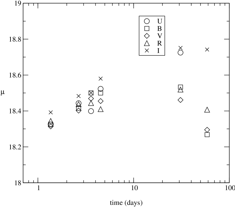
Figure 17: The distance modulus obtained from the best fit models we have calculated. The distance modulus is obtained using the photometry of Catchpole et al. (1987), Menzies et al. (1987), and Hamuy & Suntzeff (1990).

So far we have used all the model spectra presented in this paper in determining a distance. The purpose of this is to scrupulously convince the reader that we have not simply chosen models which provide us with a desired answer. However, the spirit of the SEAM method is to use only the best fit models, i.e. to use the full information of the observed SED to determine which models to include in a distance determination. If we restrict our distances to just the earliest times ($t<5$ days) where the spectra are well fit, we find $\mu=18.44\pm 0.08$ and if we limit our distances to just the best fit spectra ($t<5$ days, 31 days, 58 days) we find $\mu=18.5\pm 0.2$ using $UBVRI$, and $\mu=18.46\pm 0.12$ if we restrict ourselves to $BVRI$. Figure 17 shows the results for the SEAM distance, where we require a good fit. This result shows the advantage of the SEAM method when the quality of the fit SED to the data is evaluated to calculate distances. This should tend to reduce systematic effects when applying SEAM since the sign of the error varies with both epoch and photometric band. As our final value for $\mu$ we shall adopt the conservative $\mu=18.5\pm 0.2$, but the least scatter over the widest wavelength range leads to the slightly lower value of $\mu=18.46\pm 0.12$. Table 2 compares determinations of the distance to SN 1987A using both EPM and the ring. Our result is consistent and competitive with even the error bars of the nearly geometrical ring determination.

While the neutrino signal determines the time of the explosion of SN 1987A very accurately, it is a useful exercise to examine how the assumption of the neutrino derived time of explosion affects our models. From a $\chi^{2}$ analysis, the neutrino signal time is the “best” explosion time in that it minimizes the variance in the distance modulus, and from the SEAM analysis alone the time is known to 68% confidence ($\Delta\chi^{2}=1$) within $\delta t=\pm 0.9$ days, where the confidence intervals are symmetric about the time of the neutrino signal. Thus, the SEAM method is able to determine both the explosion date and the distance with good accuracy, although our quantitative uncertainty in the explosion time for SN 1987A likely depends on having an extremely well sampled early light curve.

4.2 Light Curves

Using our derived value of the distance modulus $\mu=18.5$, we can transform our synthetic (reddened) absolute magnitudes into (reddened) apparent magnitudes. Figure 18 compares our bolometric light curve to the results of Suntzeff & Bouchet (1990) and Bouchet et al. (1991). The early times agree quite well, although the agreement is poor for days 8-24 and then improves significantly for days $>24$. This just reflects the fact that the hydrodynamical model that we have used is not the model for SN 1987A. It is clear that days 8-24 should have a higher bolometric luminosity in order to match the observations, however we have already increased the bolometric luminosity at these times above that obtained by Blinnikov et al. (2000) and larger luminosities than we have used lead to a significantly poorer fit. Thus, there is not a one-parameter correspondence between the fit of the observed spectra to the luminosity.

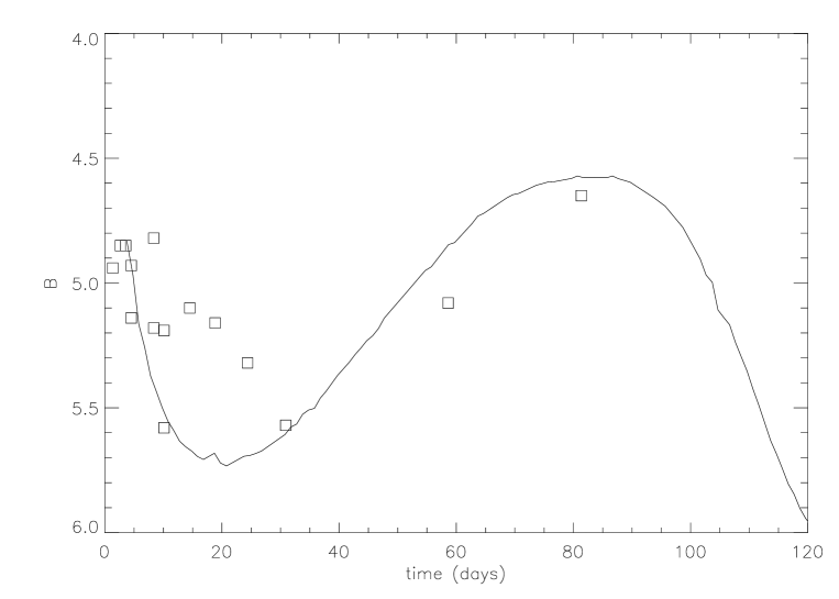
Figure 20: The observed $B$ light curve of SN 1987A (solid line Hamuy & Suntzeff, 1990) is compared with the model values (open squares).

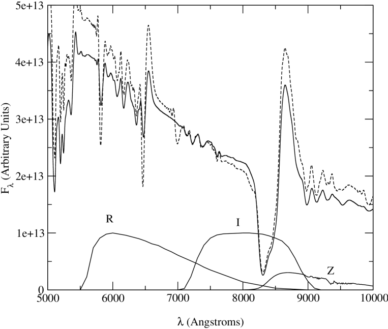
Figure 24: Two synthetic spectra for day 18 compared with the filter response for $R$, $I$, and $Z$. The synthetic spectra differ only in the total amount of nickel mixing assumed. The solid line corresponds to the self-consistent deposition function and the dashed line is for the same shape of the deposition, but multiplied by 100. Since the $I$-band doesn’t completely cover the Ca IR-triplet, it is very sensitive to the shape of the continuum around H$\alpha$ and the IR-triplet. The $Z$-band also is asymmetric about the IR-triplet.

Figures 19–23 show the optical $UBVRI$ light curves compared to the observations (Hamuy & Suntzeff, 1990). As we found in §4.1, $V$ and $R$ are most reliable and $UBI$ are less reliable, in fact $B$ fails completely. The failure in $B$ is disheartening, but shows that the $B$ band is highly sensitive to the assumed nickel distribution. Our preliminary calculations show that early $B$ band is extremely well fit in normal SNe IIP, which we believe to be better candidates for the SEAM method than are 87A-like events. The fact that $I$ is not consistent is largely due to the lack of observed spectra in the range 7000–9000 Å. If we had had spectra to fit this region we would have altered our outer boundary condition and probably achieved higher accuracy. The fact that $R$ (which includes H$\alpha$) is reasonably well reproduced is interesting. Figure 24 shows that the $I$-band only covers the absorption component of the Ca IR-triplet and is dropping in sensitivity in the emission component. The two synthetic spectra differ only in the total amount of nickel which clearly affects the shape of the continuum in addition to that of the lines. The synthetic $R$ and $I$ both differ by 0.3 mag between the two spectra, but $R-I$ differs only by 0.15 mag, so that EPM analyses that use $V-I$ to determine the color temperature might be less reliable than using $R-I$.

As we have already noted the bolometric light curve would be improved if the models were brighter in the 8-24 day epochs in particular. However, the $U$ and $B$ band light curves are too bright in this region. Thus, the density structure of the models must also be altered in order to match the observed spectra. In particular, since the blue part of the spectrum forms farthest out (due to line-blanketing from Fe II lines) it is possible that the poor fit in $U$ and $B$ is due to the atmosphere not extending to high enough velocities, thus there is not enough line blanketing. Line blanketing leads to both back warming and line cooling and so it may be possible to reduce the $U$ and $B$ magnitudes, while at the same time increasing the total bolometric luminosity. It is also possible that asymmetry is playing a role at these times, but we would expect the effects of asymmetry to increase with time and so we think that asymmetry is unlikely to be the cause here. However, the proper gamma-ray deposition function is certainly needed to reproduce the blue part of the spectrum.

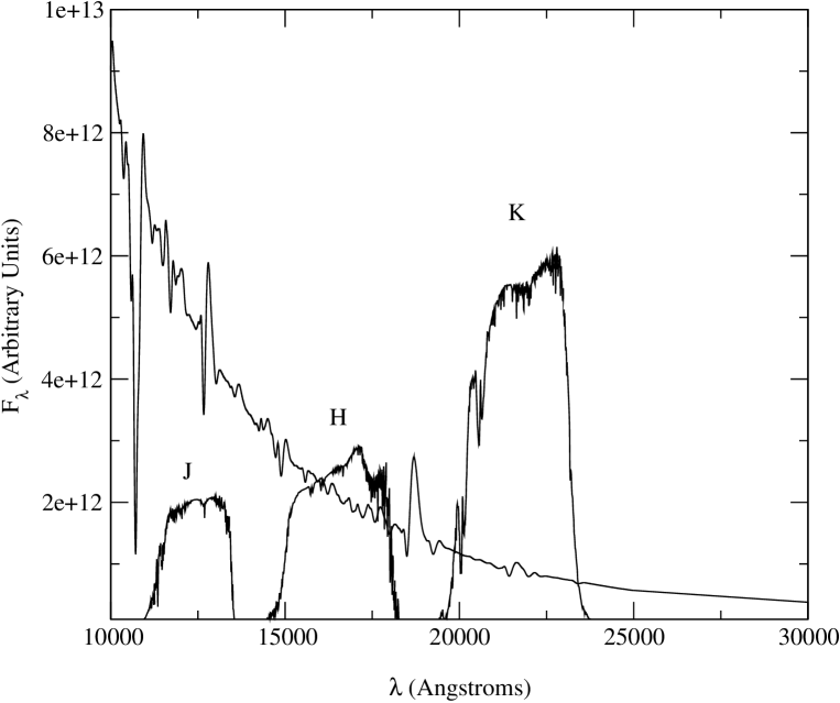
Figure 28: The spectrum of the day 30.9 model in the IR, with the filter+atmospheric transmission for $JHK$. The only prominent lines are the hydrogen lines P$\alpha$, P$\beta$, and P$\gamma$. Otherwise the SED is very close to a blackbody.

Figures 25–27 show the IR ($JHK$) light curves where even without guidance from observed spectra we obtain very good agreement. The observations are taken from Bouchet et al. (1989). This result gives us confidence in the value obtained for $\mu$ and it indicates that only small changes are needed in order to obtain consistent values of $I$. On the other hand it shows that spectroscopy in the $I$ band is required in order to obtain consistent results. Figure 28 shows the IR spectrum of the 30.9 day model with the filter and atmospheric transmission functions. The SED is nearly a blackbody with only the hydrogen lines P$\alpha$, P$\beta$, and P$\gamma$ displaying strong P-Cygni profiles.

5 Discussion

Our results indicate that the SEAM method has promise as an accurate, competitive distance indicator. It has the advantage over other methods that its results can be directly compared for consistency and that the SED includes important effects due to differential expansion and line blanketing. On the other hand, one would like to see perfect consistency in every band at every epoch. While perfect consistency is a unreachable goal, we expect improved results with early time normal Type IIP supernovae. We have used here only a single hydrodynamical model which is clearly not the model of SN 1987A. We believe that the errors can be significantly reduced with a large grid of models at each epoch which we will pursue in future work. It is particularly important to have a large range of density profiles for the lower velocity ejecta in order to correctly reproduce the Balmer lines consistently over time. It is also important for the model to extend to the highest velocity seen in the observed spectra.

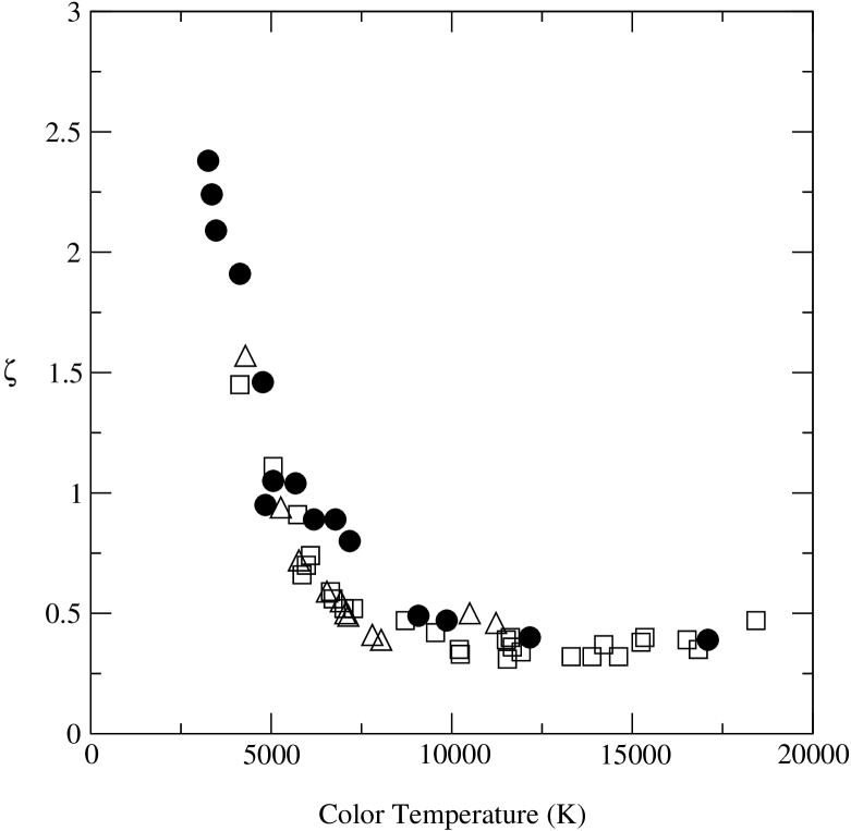
Figure 29: The dilution factor $\zeta$ from our models (filled circles) compared with that obtained by Eastman et al. (1996) for their models s15 (open squares) and p6 (open triangles).

On the face it may appear that the SEAM method is less consistent than the EPM method as applied to SN 1999em (Hamuy et al., 2001; Leonard et al., 2002). However, the EPM is more prone to systematic effects than is SEAM, where the systematic errors are more likely to average out. In EPM the “temperature” is obtained from a color temperature from different filter bands. Hamuy et al. (2001) found that the EPM leads to a deviation in the distance obtained with epoch (and they did not use either the $U$-band or $I$-band data). They also found that $BV$ were less reliable than the redder bands, which is consistent with our results. Leonard et al. (2002) found that they obtained different preferred distances when using different filter bands and that determining the velocities that are required in EPM is non-trivial. Leonard et al. (2002) found that even obtaining the rest wavelength of multiplets such as Sc II is subject to uncertainty. In reality, there is probably no single unblended line in the entire spectrum, and the problems of blending become more important for weak lines that are desired to obtain the photospheric radius. The need for detailed synthetic spectral modeling is clear. In fact, the velocity is needed in EPM not only to determine the radius of the supernova, but also to compare with models in order to obtain the dilution factor, $\zeta$. Figure 29 shows the results of our values of $\zeta$ (obtained using $BV$) with that of Eastman et al. (1996). The filled circles are our result, the triangles the power-law model, p6, of Eastman et al. (1996) and the squares the 15 ${\mathrm{M}_{\odot}}$ model, s15, of Eastman et al. (1996). There does appear to be some difference between our values and that of Eastman et al. (1996), particularly for the important color temperature range of $\sim 5000-8000$ K. Although Hamuy et al. (2001) found that the power-law model gave more consistent results for SN 1999em than s15, this cannot be physically correct since real models must flatten out at low velocity (or they would be singular).

The fact that the scatter is minimized and the fits are quite good at early times, leads us to believe that early time normal type IIP supernovae are likely the best candidates for SEAM. Since polarization is lowest at early times (Leonard et al., 2001) it is also the time that the assumption of spherical symmetry is likely to be most valid. Thus we believe that future SEAM (and EPM) analyses should concentrate on early time supernovae. It is now up to dedicated supernova searches to find supernovae at early times and to follow them both photometrically and spectroscopically.

Table 1: Mean Distance Moduli

Band	$\mu_{X}$
$U$	$18.8\pm 0.5$
$B$	$18.6\pm 0.3$
$V$	$18.5\pm 0.1$
$R$	$18.5\pm 0.1$
$I$	$18.7\pm 0.2$

Table 2: Other Distance Determinations

Distance Modulus	Distance (kpc)	Method	Source
$18.7\pm 0.2$	$55\pm 5$	EPM, $\zeta=1$	Branch (1987)
$18.2\pm 0.2$	$43.3\pm 4$	EPM	Chilukuri & Wagoner (1988)
$18.45\pm 0.25$	$49\pm 6$	EPM, $\zeta<1$	Eastman & Kirshner (1989)
$18.3\pm 0.2$	$45.3\pm 4$	EPM, $\zeta<1$	Schmutz et al. (1990)
$18.55\pm 0.12$	$51.2\pm 3.1$	ring (circular)	Panagia et al. (1991)
$<18.35\pm 0.03$	$<46.77\pm 0.76$	ring (circular)	Gould (1995)
$18.53\pm 0.07$	$50.9\pm 1.8$	ring (circular)	Panagia et al. (1997)
$18.43\pm 0.09$	$48.6\pm 2.2$	ring (circular)	Sonneborn et al. (1997)
$<18.53\pm 0.04$	$<50.8\pm 1.0$	ring (circular)	Gould & Uza (1998)
$18.44\pm 0.04$	$48.8\pm 1.1$	ring (elliptical)	Gould & Uza (1998)
$18.5\pm 0.24$	$50\pm 6$	ring (circular)	Garnavich, Kirshner, & Challis (1999)
$<18.67\pm 0.08$	$<54.2\pm 2.2$	ring (circular)	Lundqvist & Sonneborn (2001)
$18.5\pm 0.2$	$50\pm 5$	SEAM (all data)	This work
$18.46\pm 0.12$	$49.2\pm 3$	SEAM	This work

Figure 1: PHOENIX model spectrum (solid line) for day 1.36. Important optical lines include H$\alpha$ through H$\delta$, and He I $\lambda$5876. In this and following plots, all optical spectra are taken from the CTIO archive (Phillips et al., 1988) and all UV spectra are from IUE (Pun et al., 1995).

Figure 2: PHOENIX model spectrum for day 2.67. In this and subsequent figures the $1199-1227$ Å wavelength range of the IUE SWP data are saturated with geocoronal Ly$\alpha$.

Figure 3: PHOENIX model spectrum for day 3.59.

Figure 4: PHOENIX model spectrum for day 4.52, without additional nickel mixing.

Figure 5: PHOENIX model spectrum for day 4.52, with gamma-ray deposition calculated assuming local deposition due to a constant nickel mass fraction of $1.0\times 10^{-3}$ everywhere in the envelope.

Figure 6: PHOENIX model spectrum for day 8.37, with a nickel mass fraction of $1.0\times 10^{-4}$ everywhere in the envelope.

Figure 7: PHOENIX model spectrum for day 10.12, without additional nickel mixing.

Figure 9: PHOENIX model spectrum for day 14.52, with a nickel mass fraction of $1.0\times 10^{-4}$ everywhere in the envelope.

Figure 10: PHOENIX model spectrum for day 18.70, with a nickel mass fraction of $1.0\times 10^{-4}$ everywhere in the envelope, and an increase in bolometric luminosity of 25.6% from the Blinnikov et al. (2000) original value.

Figure 11: PHOENIX model spectrum for day 24.38, with a nickel mass fraction of $1.0\times 10^{-4}$ everywhere in the envelope, and an increase in bolometric luminosity of 30.9% from the Blinnikov et al. (2000) original value.

Figure 12: PHOENIX model spectrum for day 30.90, with an increase in bolometric luminosity of 36.0% from the Blinnikov et al. (2000) original value. No additional nickel mixing.

Figure 13: PHOENIX model spectrum for day 58.62, with an increase in bolometric luminosity of 28.0% from the Blinnikov et al. (2000) original value. No additional nickel mixing.

Figure 14: The UV portion of PHOENIX model spectrum for day 58.62, with an increase in bolometric luminosity of 28.0% from the Blinnikov et al. (2000) original value. No additional nickel mixing.

Figure 15: PHOENIX model spectrum for day 81.35, with an increase in bolometric luminosity of 17.5% from the Blinnikov et al. (2000) original value. No additional nickel mixing.

Figure 18: The observed bolometric light curve of SN 1987A (solid line Suntzeff & Bouchet, 1990) is compared with the model values (open squares).

Figure 19: The observed $U$ light curve of SN 1987A (solid line Hamuy & Suntzeff, 1990) is compared with the model values (open squares).

Figure 21: The observed $V$ light curve of SN 1987A (solid line Hamuy & Suntzeff, 1990) is compared with the model values (open squares).

Figure 22: The observed $R$ light curve of SN 1987A (solid line Hamuy & Suntzeff, 1990) is compared with the model values (open squares).

Figure 23: The observed $I$ light curve of SN 1987A (solid line Hamuy & Suntzeff, 1990) is compared with the model values (open squares).

Figure 25: The observed $J$ light curve of SN 1987A (solid line Bouchet et al., 1989) is compared with the model values (open squares).

Figure 26: The observed $H$ light curve of SN 1987A (solid line Bouchet et al., 1989) is compared with the model values (open squares).

Figure 27: The observed $K$ light curve of SN 1987A (solid line Bouchet et al., 1989) is compared with the model values (open squares).

References

- Baade (1926) Baade, W. 1926, Astr. Nach., 228, 359
- Baron et al. (1994) Baron, E., Hauschildt, P. H., & Branch, D. 1994, ApJ, 426, 334
- Baron et al. (1995a) Baron, E., Hauschildt, P. H., Branch, D., Austin, S., Garnavich, P., Ann, H. B., Wagner, R. M., Filippenko, A. V., Matheson, T., & Liebert, J. 1995a, ApJ, 441, 170
- Baron et al. (1996a) Baron, E., Hauschildt, P. H., Branch, D., Kirshner, R. P., & Filippenko, A. V. 1996a, MNRAS, 279, 779
- Baron et al. (1993) Baron, E., Hauschildt, P. H., Branch, D., Wagner, R. M., Austin, S. J., Filippenko, A. V., & Matheson, T. 1993, ApJ, 416, L21
- Baron et al. (1996b) Baron, E., Hauschildt, P. H., Nugent, P., & Branch, D. 1996b, MNRAS, 283, 297
- Baron et al. (1995b) Baron, E., Hauschildt, P. H., & Young, T. R. 1995b, Physics Reports, 256, 23
- Blinnikov (1999) Blinnikov, S. 1999, Astronomy Letters, 25, 359
- Blinnikov et al. (1998) Blinnikov, S., Eastman, R., Barunov, O., Popolitov, V., & Woosley, S. 1998, ApJ, 496, 454
- Blinnikov et al. (2000) Blinnikov, S., Lundqvist, P., Bartunov, O., Nomoto, K., & Iwamoto, K. 2000, ApJ, 532, 1132
- Bouchet et al. (1991) Bouchet, P., Phillips, M. M., Suntzeff, N. B., Gouiffes, C., Hanuschik, R. W., & Wooden, D. H. 1991, A&A, 245, 490
- Bouchet et al. (1989) Bouchet, P., Slezak, E., Le Bertre, T., Moneti, A., & Manfroid, J. 1989, A&AS, 80, 379
- Branch (1987) Branch, D. 1987, ApJ, 320, L27
- Branch & Patchett (1973) Branch, D. & Patchett, B. 1973, MNRAS, 161, 71
- Cardelli et al. (1989) Cardelli, J. A., Clayton, G. C., & Mathis, J. S. 1989, ApJ, 345, 245
- Catchpole et al. (1987) Catchpole, R. M., Menzies, J. W., Monk, A. S., Wargau, W. F., Pollaco, D., Carter, B. S., Whitelock, P. A., Marang, F., Laney, C. D., Balona, L. A., Feast, M. W., Lloyd Evans, T. H. H., Sekiguchi, K., Laing, J. D., Kilkenny, D. M., Spencer Jones, J., Roberts, G., Cousins, A. W. J., van Vuuren, G., & Winkler, H. 1987, MNRAS, 229, 15P
- Chilukuri & Wagoner (1988) Chilukuri, M. & Wagoner, R. V. 1988, in IAU Colloq. 108: Atmospheric Diagnostics of Stellar Evolution, 295
- Chugai (1991) Chugai, N. N. 1991, Sov. Astron. Lett., 17, 400
- Colgate et al. (1980) Colgate, S., Petschek, A., & Kriese, J. T. 1980, ApJ, 237, L81
- Eastman & Kirshner (1989) Eastman, R. & Kirshner, R. P. 1989, ApJ, 347, 771
- Eastman et al. (1996) Eastman, R., Schmidt, B. P., & Kirshner, R. 1996, ApJ, 466, 911
- Feast (2001) Feast, M. 2001, in New Cosmological Data and the Values of the Fundemental Parameters, ed. A. Lasenby & A. Wilkinson, IAU Symposium 201 (Singapore: World Scientific), in press, astro–ph/0010590
- Garnavich et al. (1999) Garnavich, P., Kirshner, R., & Challis, P. 1999, IAU circ., 7102, 1+
- Gibson (2002) Gibson, B. K. 2002, Mem. Soc. Astron. Italiana, in press, astro-ph/9910574v2
- Gould (1995) Gould, A. 1995, ApJ, 452, 189
- Gould & Uza (1998) Gould, A. & Uza, O. 1998, ApJ, 494, 118
- Groenewegen & Salaris (2001) Groenewegen, M. A. T. & Salaris, M. 2001, A&A, 366, 752
- Haas et al. (1990) Haas, M. R., Erickson, E. F., Lord, S. D., Hollenbach, D. J., Colgan, S. W. J., & Burton, M. G. 1990, ApJ, 360, 257
- Hamuy & Suntzeff (1990) Hamuy, M. & Suntzeff, N. B. 1990, AJ, 99, 1146
- Hamuy et al. (2001) Hamuy, M. et al. 2001, ApJ, 558, 615
- Hauschildt & Baron (1999) Hauschildt, P. H. & Baron, E. 1999, J. Comp. Applied Math., 109, 41
- Hauschildt & Ensman (1994) Hauschildt, P. H. & Ensman, L. 1994, ApJ, 424, 905
- Hershkowitz et al. (1986a) Hershkowitz, S., Linder, E., & Wagoner, R. 1986a, ApJ, 301, 220
- Hershkowitz et al. (1986b) —. 1986b, ApJ, 303, 800
- Hershkowitz & Wagoner (1987) Hershkowitz, S. & Wagoner, R. 1987, ApJ, 322, 967
- Höflich (1991) Höflich, P. 1991, in Proceedings of the ESO/EPIC Workshop on SN 1987A and other Supernovae, ed. I. J. Danziger & K. Kjär (Munich: ESO), 449
- Jeffery & Branch (1990) Jeffery, D. & Branch, D. 1990, in Supernovae, ed. J. C. Wheeler & T. Piran (Singapore: World Scientific), 149
- Kirshner & Kwan (1974) Kirshner, R. P. & Kwan, J. 1974, ApJ, 193, 27
- Leonard et al. (2001) Leonard, D. C., Filippenko, A. V., Ardila, D., & Brotherton, M. 2001, ApJ, 553, 861
- Leonard et al. (2002) Leonard, D. C. et al. 2002, PASP, 114, 35
- Lundqvist & Fransson (1996) Lundqvist, P. & Fransson, C. 1996, ApJ, 464, 924
- Lundqvist & Sonneborn (2001) Lundqvist, P. & Sonneborn, G. 2001, in SN 1987A: Ten Years After, ed. M. Phillips & N. Suntzeff, Vol. in press, astro-ph/9707144 (San Francisco: ASP)
- McCall (1993) McCall, M. L. 1993, ApJ, 417, L75
- Menzies et al. (1987) Menzies, J. W., Catchpole, R. M., van Vuuren, G., Winkler, H., Laney, C. D., Whitelock, P. A., Cousins, A. W. J., Carter, B. S., Marang, F., Lloyd Evans, T. H. H., Roberts, G., Kilkenny, D., Spencer Jones, J., Sekiguchi, K., Fairall, A. P., & Wolstencroft, R. D. 1987, MNRAS, 227, 39P
- Mitchell et al. (2001) Mitchell, R., Baron, E., Branch, D., Lundqvist, P., Blinnikov, S., & Hauschildt, P. H. 2001, ApJ, 556, 979
- Nagataki (2000) Nagataki, S. 2000, ApJS, 127, 141
- Nomoto & Hashimoto (1988) Nomoto, K. & Hashimoto, M. 1988, Phys. Repts., 163, 13
- Panagia et al. (1991) Panagia, N., Gilmozzi, R., Macchetto, F., Adorf, H.-M., & Kirshner, R. P. 1991, ApJ, 380, L23
- Panagia et al. (1997) Panagia, N. et al. 1997, in BAAS, Vol. 191, 1909
- Phillips et al. (1988) Phillips, M., Hamuy, M., Heathcote, S., Suntzeff, N., & Kirhakos, S. 1988, AJ, 95, 1087
- Pun et al. (1995) Pun, C. S. J. et al. 1995, ApJS, 99, 223
- Saio et al. (1988) Saio, H., Kato, M., & Nomoto, K. 1988, ApJ, 331, 388
- Saio et al. (1988) Saio, H., Nomoto, K., & Kato, M. 1988, Nature, 334, 508
- Schmidt et al. (1992) Schmidt, B. P., Kirshner, R., & Eastman, R. 1992, ApJ, 395, 366
- Schmutz et al. (1990) Schmutz, W., Abbott, D. C., Russell, R. S., Hamann, W.-R., & Wessolowski, U. 1990, ApJ, 355, 255
- Short et al. (1999) Short, C. I., Hauschildt, P. H., & Baron, E. 1999, ApJ, 525, 375
- Sonneborn et al. (1997) Sonneborn, G. et al. 1997, ApJ, 447, 848
- Suntzeff & Bouchet (1990) Suntzeff, N. B. & Bouchet, P. 1990, AJ, 99, 650
- Swartz et al. (1995) Swartz, D., Sutherland, P., & Harkness, R. 1995, ApJ, 446, 766
- Takeda (1991) Takeda, Y. 1991, A&A, 245, 182
- Tonry (2001) Tonry, J. 2001, in Astrophysical Ages and Time Series, ed. T. von Hippel, N. Manset, & C. Simpson (San Francisco: ASP)
- Utrobin & Chugai (2002) Utrobin, V. P. & Chugai, N. N. 2002, Astronomy Letters, in press
- Williams (1987) Williams, R. E. 1987, ApJ, 320, L117