On the accuracy of the S/N estimates obtained with the exposure time calculator of the Wide Field Planetary Camera 2 on board the Hubble Space Telescope

Abstract

We have studied the accuracy and reliability of the exposure time calculator (ETC) of the Wide Field Planetary Camera 2 (WFPC2) on board the Hubble Space Telescope (HST) with the objective of determining how well it represents actual observations and, therefore, how much confidence can be invested in it and in similar software tools. We have found, for example, that the ETC gives, in certain circumstances, very optimistic values for the signal-to-noise ratio (SNR) of point sources. These values overestimate by up to a factor of 2 the HST performance when simulations are needed to plan deep imaging observations, thus bearing serious implications on observing time allocation. For this particular case, we calculate the corrective factors to compute the appropriate SNR and detection limits and we show how these corrections vary with field crowding and sky background. We also compare the ETC of the WFPC2 with a more general ETC tool, which takes into account the real effects of pixel size and charge diffusion. Our analysis indicates that similar problems may afflict other ETCs in general showing the limits to which they are bound and the caution with which their results must be taken.

1 Introduction

ETCs play an important role in modern instrument use as they allow observers to determine how to carry out specific investigations and, especially, to predict the amount of time these will require. Since the time needed for the various programmes is a very sensitive issue in the allocation process for most modern high visibility ground and space-based facilities, the accuracy of these simulators must be well understood both by the observers and the time allocation committees that must rely on their results for a fair and scientifically effective distribution of the available time. In this context, unfortunately, besides the documentation accompanying the software tools, there is practically no published information on the reliability of existing ETCs of imaging cameras.

The WFPC2 has been so far the principal instrument on board the HST and it is expected to be of extreme utility to image parallel fields even now that the Advanced Camera for Surveys (ACS) is installed on the HST. ETC software utilities are available on the internet site of the STScI which simulate analytically the photometry for a given target for each HST instrument. The accuracy of these programmes plays a fundamental role in the planning of observations, in particular when extremely deep imaging is required and whenever the performances of two different instruments have to be compared.

While performing simulations for an HST proposal for the WFPC2 and the ACS, in which high accuracy was needed in order to evaluate the limiting magnitudes for deep observations of a globular cluster, we found substantial differences between the WFPC2 ETC results and real photometry obtained on archival images. We found similar differences also in archival non crowded fields, so that we decided to analyse the problem by directly comparing the ETC predictions with our photometry in various circumstances and here we show the results and the way in which they depend on field crowding. We also compare our photometry with the result of the recently published “ETC++” software (Bernstein, 2001), whose calculations are based on statistical analysis tools and take into account the real effects of the pixel size and charge diffusion.

2 The WFPC2 ETC: comparison with real point–source photometry

The WFPC2 ETC computes the expected SNR of a point source from its input parameters, namely: the magnitude of the star in a given spectral band, the spectral type, the filter to use, the channel of the detector (PC1 or WF2, WF3, WF4), the analogue to digital gain, the position of the star on the pixel (centre or corner), the exposure time of the whole observation (i.e. the sum of all the exposure frames) and the sky coordinates of the target (Biretta, 1996). As of late, the option to manually select a specific value of the sky brightness has been added (Biretta, 2001).

First, the programme computes the source count rate, assuming a blackbody spectrum, if the user has not specified it, and multiplies it by the response curves of the detector and filter. Then, the programme takes into account the various noise sources, including photon noise, read noise, dark noise and sky noise. The latter depends on the target position on the sky, with the sky brightening by about one magnitude from the ecliptic pole to the ecliptic plane. The programme uses the values from Table 6.4 in the WFPC2 Instrument Handbook (Biretta & Heyer, 2001) to compute the sky count rate per pixel and hence its photon noise. The contribution of the total noise to the photometry of a star depends upon the number of pixels in the point spread function (PSF) and how these pixels are weighted during data reduction. The WFPC2 ETC assumes that the data reduction employs PSF fitting photometry, so that it weights the pixels in proportion to their intensity, which maximises the SNR. The multiple read errors for a “cosmic–ray splitted” (CR-split) image, i.e. an image composed by many shorter frames, is then computed for a set of default splitting values and the corresponding SNR is also given in the ETC result page.

In order to quantify the possible WFPC2 ETC deviations from real photometry, we performed accurate aperture photometry (using the DAOPhot package) on both crowded and non crowded archival fields. The average image used in our analysis was computed after aligning the individual frames in the dithering pattern and removing cosmic ray hits. A custom programme was used, which computes the offsets of the frames by measuring the mean displacement of the centroid of some reference stars. The task then registers all the images to the first one, creates a mask of the CR-contaminated pixels, by means of an iterative sigma clipping routine with respect to the median value of the corresponding pixels in all frames, and finally computes the mean image by averaging the corresponding pixel on all the images if not included in the CR-mask. The CR-corrupted pixel in the original un-shifted frames are also replaced by the value of the corresponding pixel in the mean image in order to allow us to perform photometry on both the combined and on the individual frames. Our instrumental magnitudes were then transformed to the Johnson/Cousin UBVRI system by following the prescription of (Holtzmann et al., 1995) — specifically, their equation 8, which also takes account of the colour correction by means of the coefficients in Table 7 therein — and by making an optimal choice of the aperture radius for each star, so as to minimise the associated photometric error.

For the crowded field, we have used the images of the Galactic globular cluster $M\,4$ (HST proposal 5461), obtained in the F555W and F814W filters. These are deep images centered in a region at one core radius from the centre of a dense globular cluster and should be representative of the cases in which the field observed is filled with a multitude of very bright and saturated stars ($V\leq 16$), whose haloes overlap each other and cover a significant fraction of the frame (Figure 1).

Images of the field of ARP 2 taken from HST proposal 6701, also obtained through F555W and F814W filters, were used as representative of a sparsely filled region in which the field is populated with faint stars with no appreciable overlapping haloes (Figure 2).

2.1 How we measured the SNR

Aperture photometry was performed on both series of images (i.e. crowded and non crowded), with the following parameters. The flux of the object was sampled within an aperture of radius $r_{0}$, which is varied in steps of $0.5$ pixel. The background is sampled within an annulus drawn from an inner radius $r_{1}=r_{0}+1$ pixel to an outer radius $r_{2}$, with an annulus width which is varied from $3$ pixel up to $20$ pixel. As is discussed later in this section, an adjustable aperture radius and annulus size allow us to maximise the SNR, by limiting the noise generated by the contamination of the neighbouring objects. Moreover, the background is always estimated by taking the mode, rather than the mean or median, of the pixel distribution within the annulus. Appropriate aperture corrections were applied, which were directly measured from the most isolated non saturated stars in the field. A direct comparison with the encircled energy curve for the WFPC2 PSF (Biretta & Heyer, 2001) shows a perfect match, thus proving that the growth curves that we measured are reliable.

The DAOPhot task, used with the optimal aperture radius $r_{0}$ and the radii $r_{1}$ and $r_{2}$ for the sky annulus, gives the best estimate of both the magnitude and the associated error $\sigma_{m}$, from which we compute the SNR by using the equation:

$${\rm SNR^{D}}=\frac{1}{{\rm e}^{-\sigma_{m}/1.08574}-1}$$ (1)

that comes from inverting Pogson’s relation $\Delta m=-2.5\,{\rm log}((F+\Delta F)/F)$, where the numerical constant $1.08574$ is equal to $2.5\,{\rm ln}(10)$. Hereafter, the acronym ${\rm SNR^{D}}$ indicates the SNR estimated on the basis of the photometric error given by DAOPhot.

As an independent check, we have computed the SNR as indicated in equation 6.7 of the WFPC2 Handbook (Biretta & Heyer, 2001) which, in the practical case of observed quantities, becomes:

$${\rm SNR^{H}}=\frac{F\cdot G^{1/2}\cdot N^{1/2}}{\sqrt{F+(S+N_{R}^{2}/G)\cdot\pi\cdot r_{0}^{2}+N_{S}}}$$ (2)

where $r_{0}$ is the optimal aperture radius used by DAOPhot, $N$ is the number of frames combined together, $N_{R}$ the read-out noise (in units of electrons) of each specific CCD, $S$ the average background per pixel inside the annulus from $r_{1}$ to $r_{2}$, in units of DN, $F$ is the flux within the aperture of radius $r_{0}$ after subtraction of the background contribution $S\cdot\pi\cdot r_{0}^{2}$, in units of DN, and $G$ is the effective gain factor, i.e. the CCD gain times the number of frames averaged togheter. Finally, $N_{S}$ is a small (although non negligible) contribution to the error affecting the estimate of the background level which takes on the form:

$$N_{S}=\frac{(S+N_{R}^{2}/G)\cdot\pi\cdot r_{0}^{4}}{r_{2}^{2}-r_{1}^{2}}$$ (3)

The computation of ${\rm SNR^{H}}$ makes no use of the error estimate on the magnitude or flux provided by DAOPhot, so it is reassuring to find that ${\rm SNR^{H}}$ is in excellent agreement with ${\rm SNR^{D}}$. This, however, only happens if we use an adaptive choice for aperture radius and for the background annulus, as explained above. In fact, if we select a fixed radius and annulus size in a crowded environment, the contamination due to neighbouring stars alters the statistics of the sky within the annulus and we always find ${\rm SNR^{H}}>{\rm SNR^{D}}$. This is precisely the reason that made De Marchi et al. (1993) conclude that core aperture photometry, i.e. source and sky measurement conducted as close to the source as possible, as well as the use of the mode for the background are most advisable in crowded environments.

2.2 How the ETC expects the SNR to be measured

In light of the consistency between ${\rm SNR^{D}}$ and ${\rm SNR^{H}}$ and since the latter stems directly from equation 6.7 of the WFPC2 Handbook, on which the WFPC2 ETC is also based, we can now proceed and compare our measured ${\rm SNR^{D}}$ with the ETC predictions. Before doing so, however, we must make sure that the way in which we measure the SNR (i.e. ${\rm SNR^{D}}$) is consistent with the way in which the ETC software expects users to carry out the photometry. In fact, the latter assumes that the data reduction process employ PSF fitting photometry, i.e. that optimal weighting be assigned to each pixel in proportion to its intensity in the PSF. As discussed above, however, we have used aperture photometry to determine ${\rm SNR^{D}}$. The WFPC2 ETC instructions would indeed offer a correction to apply to the ideal PSF fitting case ${\rm SNR^{P}}$ (we call it “ETC optimal SNR”) in order to convert it to the equivalent SNR that would be obtained with canonical aperture photometry ${\rm SNR^{A}}$ (“ETC aperture SNR”). Following the WFPC2 ETC instructions in (Biretta, 1996), we have:

$${\rm SNR^{A}}={\rm SNR^{P}}\cdot\frac{K}{r_{0}}$$ (4)

where $K=0.11$ for the PC camera and $K=0.17$ for the WF chips, particularly valid when the aperture radius is $r_{0}>2.5$ pixel for the PC and $r_{0}>1.8$ pixel in the case of the WF.

Since we determined ${\rm SNR^{D}}$ by using aperture photometry, it would seem that we need to take into account the correction given by Equation 4. We show, however, that this correction is not necessary thanks to the adaptive method that we used for photometry. In Figure 3 we plot, for the PC chip, the measured ${\rm SNR^{D}}$ against the prediction of the ETC for the aperture photometry case, i.e. ${\rm SNR^{A}}$. We should like to clarify here how Figure 3 and others of the same type in the following were built. After having measured the calibrated magnitude of a star in the images, we folded the latter value through the WFPC2 ETC so as to calculate the estimated SNR for an object of that brightness and for the exposure time and CR-SPLIT pattern corresponding to those of the actual combined image. For this and all the other figures in this paper, unless otherwise specified, we used the “average sky” option for the sky brightness setting as allowed by the new WFPC2 ETC Version 3.0.

We can see from Figure 3 that the prediction of the ETC for aperture photometry (${\rm SNR^{A}}$) are over-estimated for faint stars and under-estimated for bright objects with respect to the measured values for both the sparse and the crowded field. Figure 4 is the analogue of Figure 3 but here the reference is the ETC optimal SNR, ${\rm SNR^{P}}$, i.e. without any correction for aperture photometry. As one can easily see, the ETC in this case always overestimates the value of the SNR with respect to the measured ones by up to $\sim 100\,\%$ for the fainter stars. As the right hand side axis shows, such a mismatch of the SNR corresponds to a time estimation error of the same amount (see Equation 7 ahead), i.e. the ETC appears to underestimate the exposure time actually needed to achieve a given SNR.

A closer look at Figure 4, however, reveals that the scatter of the representative points on the plot is smaller when our measurements are compared with SNR^P than for SNR^A and that the overall behaviour is closer to the ETC prediction at any magnitude. This is a consequence of our optimised aperture and annulus photometry closely approaching PSF fitting. In light of these results, in the following we ignore the correction for aperture photometry given by equation 4 and compare our measurements directly with the ETC optimal SNR, i.e. SNR^P.

2.3 How the predicted SNR compares with the observed one

Figures 3 and 4 clearly witness the dependence of the actual SNR upon the level of field crowding and, at the same time, its independence of the filter used. In principle, one could question the validity of our latest assumption, i.e. that of ignoring the correction to be applied to the SNR measured with aperture photometry. In fact, in a crowded field, PSF fitting photometry is expected to give better results. We have, therefore, attempted a direct comparison between the predictions of the ETC and the results of PSF fitting photometry. Rather than carrying out the reduction ourselves, we have utilised one of the finest examples of photometric work carried out on these very M 4 data by Richer et al. (1997), who employed very accurate ALLFRAME photometry as described in detail in Ibata et al. (1999). In their paper, these authors measure the magnitude of each star from the individual frames in the dithering stack and compute the combined magnitudes as the weighted average of the corresponding fluxes, the error on them, $\sigma_{m}^{P}$, being related to the flux scatter amongst the frames.

In order to make a reliable comparison with our results, we have performed, in a similar way, optimised aperture photometry on the individual frames (i.e. the original, not yet aligned images, in which CR-hits had been removed as described above). The measured fluxes were averaged with a weight inversely proportional to the DAOPhot estimated uncertainty after rescaling for the flux ratio. Our final magnitude errors, $\sigma_{m}^{A}$, are thus derived from the standard deviation of the fluxes, divided by the square root of the number of images combined. Figure 5 displays the comparison between $\sigma_{m}^{P}$, $\sigma_{m}^{A}$ and the ETC prediction, showing that the two photometric uncertainties overlap each other, while the ETC largely overestimates the precision that can be attained with PSF fitting photometry, even by one of the most experienced teams.

Thus, in this crowded case, it is also apparent that the ETC deviations are independent of the photometric technique adopted. In sparse fields, where aperture photometry and PSF fitting are equally effective and reliable, Figures 3 and 4 already prove that the ETC predictions depart from the measured data, although by a smaller amount than that applicable in the crowded case. Finally, in Figure 6 we compare the predictions of the ETC with the actual measurements for both the PC and WF, to show that the behaviour of the ETC applies regardless of the channel.

The relevance of the above considerations becomes clear when one uses an ETC to simulate very deep observations, especially when a comparison between instruments, e.g. ACS/WFC and WFPC2, is required to compare the limiting magnitude in given exposure times. As experience shows, a star finding programme is able to detect a faint point source only when its brightest pixel is at least $2$ or $3\,\sigma_{\rm sky}$ above the sky background (where $\sigma_{\rm sky}$ is the standard deviation of the background), with a value of $\sim 5$ or more being the typical prerequisite in most faint photometry precision applications. If we plot the so called object detectability $d$, defined as:

$$d=\frac{\rm Peak-Sky}{\sigma_{\rm sky}}$$ (5)

as a function of the magnitude error $\sigma_{m}$, we obtain the graph in Figure 7. Here we notice that the detectability (which is practically independent of the filter and crowding) drops to the value of $d=2.1$ just when the magnitude error approaches $0.5\,mag$, which is usually considered the maximum allowed error in canonical photometric work. By relating the detectability $d$ with the ETC optimal SNR, ${\rm SNR^{P}}$, as done in Figure 8, we see that $d=2.1$ corresponds to an ETC optimal SNR of $3.0$ for the non crowded case and to $7.0$ for the crowded case. This literally means that if we need to know the magnitude of the faintest detectable star in an observation of a stellar field with the WFPC2 we should query the ETC, setting “average sky”, for a SNR of $7.0$ and $3.0$, respectively in a crowded and in a sparse environment. It is normally assumed that a $3\,\sigma$ detection requires a SNR of 3, but in the case of the SNR provided by the WFPC2 ETC, this is only true for an isolated object.

3 Discussion and corrections

The direct consequence of what we have illustrated so far is that, if the ETC were used to plan observations of faint stars in a globular cluster like M 4 with the WFPC2, the predicted exposure time could be considerably underestimated. Conversely, the same predictions would be almost correct for a star of equal brightness in a sparse field. In the following we try and provide an empirical correction formula that can be applied to the SNR given by the WFPC2 ETC to compensate for the effects of crowding.

In order to understand the discrepancy between the expected and measured SNR and to clarify how to exactly account for the effects of crowding in the simulations, we artificially modified the background level and photon noise in the sparse field so as to reproduce the sky level and sky variance measured on the crowded field. In practice, we added to the sparse field a Gaussian noise with a mean equal to the difference in the sky level between the two fields and a variance equal to the quadratic difference of the sky variances between them. The SNR diagramme for the modified image (Figure 9) reveals that the locus of the modified sparse data points shifts towards and perfectly overlaps the crowded field locus. This tells us, as expected, that the increased background level resulting from crowding is responsible for the differences shown in Figures 3 and 4 between sparse and crowded fields.

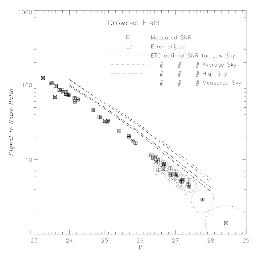
Figure 10: Comparison between the measured SNR (SNR^D) and the ETC predictions for i) default low background, ii) default average background, iii) default high background and iv) actually measured background.

It is, however, true that the ETC gives the SNR under the best possible sky conditions, which are rarely encountered, if ever, in real observations. Moreover, it is generally not expected of the ETC to take account of the position and brightness of all the stars in the field as would be necessary to simulate how crowding increases the background level. We have, therefore, manually set the ETC sky brightness to match the levels directly measured with the DAOPhot SKY task on the crowded image (i.e.. the mode of the levels distribution), hoping in this way to force the SNR simulated by the ETC to agree with our measurements. In fact, the results change only marginally, as shown in Figure 10, where ${\rm SNR^{D}}$ and ${\rm SNR^{P}}$ are plotted against the observed magnitude (Johnson $V$ in this case). The ETC simulation gets closer to the real data, but it does not still match them. Moreover, it seems as if a suitable value for the background cannot be found at all as shown in Figure 11, where one sees that the sky value that would force the ETC prediction to match ${\rm SNR^{D}}$, changes significantly as a function of star brightness.

We must, thus, conclude that the treatment of the background is a major issue for the WFPC2 ETC, although that alone cannot explain the whole discrepancy. It goes without saying that we have verified and confirmed that the predictions of the ETC as concerns the count rates per pixel in the source and background are precise to within an accuracy of 10 %, as one would expect of a professional tool. We have also repeated all our tests on the individual frames, compared in turn with the predictions of the ETC for a case of CR-SPLIT=1. The result being the same, we can exclude an error in either the way in which we combined the data or in the way in which the ETC accounts for CR-SPLIT$>1$. The rest of the discrepancy, then, must be attributed to the way in which the noise is estimated, the signal being correct. A delicate issue could be, for instance, the value and operational definition of $\sigma_{\rm sky}$. We notice here that large variations in the value of $\sigma_{\rm sky}$ are possible, in the crowded environment, depending as to whether we measure it with the IRAF SKY task, which fits a Gaussian around the mode, or as the standard deviation that one obtains by manual analysis over the darkest regions of the background in the image. In fact the latter can be up to 3 times smaller than the former, and also 2 times smaller than the mean sigma as measured inside the photometric sky annulus around each star. Conversely, all these numbers turn out to be quite similar for the sparse field image.

To try and account for the possible sources of the residual error, we considered recent results published by Bernstein (2001), who uses Fourier analysis and Fisher information matrices to show to which extent the SNR of a point source depends on factors which normally are not considered in ETC programmes, such as pixel size, intra-pixel response function, extra-pixel charge diffusion and cosmic ray hits.

According to this work, a programme that does not take all these parameters into account may overestimate the SNR by up to a factor of 2. More precisely, whenever background limited point source photometry is involved, the key factor for the SNR calculation, namely the “effective area” $A_{SN}$ (see equation 12 in Bernstein 2001), strongly depends on the detector geometry, such as pixel size, under-sampling factor, intra-pixel response function and charge diffusion. The finite pixel size plays an important role, as even a Nyquist sampled pixel (i.e. one $\lambda/2D$ in size) causes a 13 % degradation in the SNR of a faint star and the same applies to extra-pixel charge diffusion.

In order to check whether these problems also affect the WFPC2, we configured Bernstein’s “ETC++” software to simulate WFPC2 point source photometry for the sparse field. The result is shown in Figure 12 where the measured SNR (${\rm SNR^{D}}$), the ETC optimal SNR (${\rm SNR^{P}}$) and the ETC++ SNR for aperture photometry are plotted against the stellar magnitude. The ETC++ gives a confidence level for its results as the value of the cumulative function of the stars distribution above the computed SNR. The ETC++ line in Figure 12 means that 50 % of the stars of any given magnitude should be above this line. The WFPC2 ETC does not give confidence levels, but we can assume that its SNR is computed as the mean of the SNR distribution at any given magnitude, i.e. at 50 % confidence level. If this is the case, Figure 12 indicates that the actual SNR is located in between the WFPC2 ETC and the ETC++ predictions, thus confirming the difficulty of any analytical ETC in reliably estimating the SNR.

Thus, a correction for the currently on-line WFPC2 ETC can only be empirical in nature. The following formula can be used to obtain a realistic estimate of the SNR:

$${\rm SNR^{C}}\simeq(60\cdot C+17)\cdot(e^{-0.012\cdot{\rm SNR^{P}}}-1)+0.93\cdot{\rm SNR^{P}}$$ (6)

where ${\rm SNR^{P}}$ is the SNR estimated by the ETC without correction for aperture photometry and $C$ is a measure of the crowding, defined as the logarithm of the ratio between the total area of the chip and the number of pixel with value lower than the modal sky value plus one standard deviation. For example $C$ is equal to $0.05$ for our sparse field, whereas it grows to $0.42$ in the crowded case of M 4. For faint stars, e.g. for ${\rm SNR^{P}}\lesssim 20$, this equation can be roughly approximated by the rule of thumb that the actual SNR is about $1/2$, or $2/3$, of the ${\rm SNR^{P}}$, respectively for a crowded and non crowded environment. It should be noted that not even in an ideal case of zero crowding ($C\simeq 0$) would the measured SNR match the prediction of the ETC, since there would still be a discrepancy of the same order of that found in the sparse case.

The advantage of this formula is that ${\rm SNR^{C}}=3$ would now always imply a $3\,\sigma$ detection, regardless of the level of crowding in the image. The correction that we propose would allow an observer to accurately plan his observations and make the best use of the HST time. For the low SNR regime (e.g. ${\rm SNR^{P}}\lesssim 50$), equation 6 can actually be rewritten to more explicitly show the effects of crowding on the exposure time:

$${\rm t^{C}}\simeq{\rm t^{P}}\cdot\frac{{\rm SNR^{P}}}{(60\cdot C+17)\cdot(e^{-0.012\cdot{\rm SNR^{P}}}-1)+0.93\cdot{\rm SNR^{P}}}$$ (7)

where ${\rm t^{P}}$ is the exposure time predicted by the ETC to reach a certain SNR and ${\rm t^{C}}$ is its actual value.

An example of how serious the underestimate of the exposure time can be when the ETC is not used with the above caveat in mind is given in Figures 13a and 13b for a crowded environment. There we show a simulation of the detectability of the white dwarf cooling sequence with the WFPC2 in NGC6397, the nearest globular cluster, through the filters F606W and F814W. We have adopted the theoretical WD cooling sequence of Prada Moroni et al. (2002) which provide a perfectly thin isochrone and have applied to it the colour and magnitude uncertainty that one obtains from the estimated SNR by inverting equation 1. Two cases are shown: one (a) as predicted by the WFPC2 ETC and one (b) for our corrected estimate of equation 6. The difference is outstanding, as the ETC predictions, taken at face value and ignoring the effects of crowding, would suggest that the sequence is not spread very much by photometric errors and its quasi-horizontal tail between $m_{606}=29$ and $m_{606}=30$ is clearly noticeable, whereas in our realistic simulation the sequence is widely spread and its lower part lies well below the detection limit.

The delicacy of the issue is immediately apparent when one considers that, based on the ETC estimates, one would deem that 120 orbits are sufficient to reliably secure the white dwarf cooling sequence in the colour–magnitude diagramme of NGC6397 down to $m_{606}=30.5$ and $m_{814}=30$, whereas, in fact, the correction shows that as many as 255 orbits would be needed to comfortably reach those limits with the WFPC2.

All of the above considerations are valid not only for the WFPC2, but also for any analytical ETC in general, especially when used to estimate the SNR of stars embedded in crowded environment or when the detector considerably under-samples the PSF, as suggested in Bernstein (2001). We should underline here, however, that this does not mean at all that the ETCs are unreliable nor that they are useless. One of the most important and practical reasons for having a standardised ETC is to allow the telescope time allocation committees to compare all the proposals on equal footing. In this respect, the ETC does not necessarily need to be accurate. Clearly, the better the detector’s cosmetics, intra-pixel response, charge diffusion and readout noise, the closer will the real photometry be to the ETC prediction. Thus, we expect, for example, a better behaviour of the ACS/WFC on-line simulator with respect to the WFPC2.

A non-analytical SNR calculator, which would simulate the whole observing session, including the dithering pattern, by numerically reproducing the real field (i.e. with the correct stellar positions and brightness, as imaged by a realistic model of the detector) and which uses the same photometric tools that will be adopted by the user (such as DAOPhot, ALLSTAR, and the like), would be, in our opinion, the best method to accurately predict the expected performances of any planned observing programme providing reliable results. Alternatively, at least for imaging ETCs which have very few configuration parameters and are fairly stable such as those in space telescopes, one should consider empirical modeling. One can take real results, such as we did in this paper, to calibrate an ETC which in turn interpolates between calibrations. In this way, the use of an empirical correction formula such as the one proposed here would guarantee a closer matching between simulations and real observations.

4 Summary and conclusions

The results of the WFPC2 exposure time calculator for point sources have been analysed by direct comparison with aperture and PSF photometry on real archival images. Significant deviations have been found between the ETC predictions and the actual photometry on the real data. Specifically, the analysis shows that the ETC deviations are i) independent of the filter, ii) independent of the choice of optimised aperture photometry or PFS fitting photometry, iii) independent of the PC or WF channel used, iv) strongly dependent upon the level of crowding in the field and that v) the ETC systematically overestimates the SNR, slightly for the bright sources and more seriously for faint sources close to the detection limit. Moreover, when data reduction follows the optimised aperture photometry method, the measured SNR will be as good as that obtained with PSF fitting and there is no need to apply the aperture photometry conversion suggested in the ETC documentation. An empirical correction formula is given to compute realistic SNR estimates, so as to assist observation planning when extremely faint sources have to be imaged, an example of which is presented. Manually increasing the value of the sky brightness in the simulator, so as to mimic the effects of crowding, shows that, although important, the background level is not the key parameter to explain the discrepancy, which is present even for data collected in rather sparse environments. Thus, it is not possible to correct the WFPC2 ETC predictions by just modifying the sky level. A comparison with a software tool developped by Bernstein (2001), whose predictions slightly underestimate the SNR at variance with the WFPC2 ETC, suggests that the effects of pixel size, charge diffusion and cosmic rays hits could be more important than previously thought.

FIGURE CAPTIONS:

Figure 1: Negative image of a crowded field in the globular cluster M4 obtained with the PC channel of the WFPC2 through the F555W filter (Richer et al., 1997).

Figure 2: Negative image of a sparse field obtained with the PC (Ibata et al., 1998).

Figure 3: The ratio between the SNR measured in crowded and sparse fields (SNR^D in the text) and the WFPC2 ETC prediction for aperture photometry (SNR^A in the text) is shown for the F555W and F814W filters.

Figure 4: The ratio between the SNR measured in crowded and sparse fields (SNR^D in the text) and the WFPC2 ETC prediction for PSF-fitting photometry (SNR^P in the text) is shown for the F555W and F814W filters. The right hand side axis applies to the low SNR regime ($\lesssim 50$) and indicates the amount of the time estimation error, i.e. the ratio between the actual exposure time (Equation 7 in the text) and that estimated by the ETC, for a given SNR in the abscissa.

Figure 5: Measured magnitude error from PSF-fitting photometry of Ibata et al. (1999) ($\sigma_{m}^{P}$) and from our optimized aperture photometry ($\sigma_{m}^{A}$), as a function of the magnitude, compared with the WFPC2 ETC prediction, for the crowded field and F555W filter.

Figure 6: The ratio between the measured SNR (SNR^D) and the ETC optimal SNR (SNR^P) is shown for the PC and the WF2 channels of the WFPC2, in the crowded field case.

Figure 7: Detectability $d$ versus measured magnitude error ($\sigma_{m}$). An uncertainty $\sigma_{m}=0.5mag$, usually the highest allowed in most photometric works, corresponds to a detectability $d=2.1$.

Figure 8: Detectability $d$ versus ETC optimal SNR (SNR^P). A value of $d=2.1$ corresponds to a detection limit of $SNR^{P}=3.0$ or $SNR^{P}=7.0$ respectively for the sparse and the crowded case.

Figure 9: The ratio between the measured SNR (SNR^D) and the ETC optimal SNR (SNR^P) is shown for the crowded and sparse fields, before and after the artificial brightening of the sparse field background.

Figure 11: Values to enter in the User Specified Sky Background parameter of the WFPC2 ETC in order to force the ETC to match the measured SNR for crowded and non crowded fields.

Figure 12: Comparison between the prediction of the WFPC2 ETC v.3.0, the prediction of the ETC++ software and the measured SNR (SNR^D), for the crowded and non crowded cases in the two filters (both ETCs were used here after setting the sky magnitude to the value measured in the real images).

Figure 13: Comparison between (a) the WFPC2 ETC predictions (SNR^P) and (b) our correction of equation 6 (SNR^C), in a simulation of a 120 HST orbits observation of the white dwarfs cooling sequence in NGC6397, in a colour–magnitude diagramme made through the filters F606W and F814W.

Figure 1: Negative image of a crowded field in the globular cluster M4 obtained with the PC channel of the WFPC2 through the F555W filter (Richer et al. (1997)).

Figure 2: Negative image of a sparse field obtained with the PC (Ibata et al. (1998)).

Figure 3: The ratio between the SNR measured in crowded and sparse fields (SNR^D in the text) and the WFPC2 ETC prediction for aperture photometry (SNR^A in the text) is shown for the F555W and F814W filters.

Figure 4: The ratio between the SNR measured in crowded and sparse fields (SNR^D in the text) and the WFPC2 ETC prediction for PSF-fitting photometry (SNR^P in the text) is shown for the F555W and F814W filters. The right hand side axis applies to the low SNR regime ($\lesssim 50$) and indicates the amount of the time estimation error, i.e. the ratio between the actual exposure time (Equation 7 in the text) and that estimated by the ETC, for a given SNR in the abscissa.

Figure 5: Measured magnitude error from PSF-fitting photometry of Ibata et al. (1999) ($\sigma_{m}^{P}$) and from our optimized aperture photometry ($\sigma_{m}^{A}$), as a function of the magnitude, compared with the WFPC2 ETC prediction, for the crowded field and F555W filter.

Figure 6: The ratio between the measured SNR (SNR^D) and the ETC optimal SNR (SNR^P) is shown for the PC and the WF2 channels of the WFPC2, in the crowded field case.

Figure 7: Detectability $d$ versus measured magnitude error ($\sigma_{m}$). An uncertainty $\sigma_{m}=0.5mag$, usually the highest allowed in most photometric works, corresponds to a detectability $d=2.1$.

Figure 8: Detectability $d$ versus ETC optimal SNR (SNR^P). A value of $d=2.1$ corresponds to a detection limit of $SNR^{P}=3.0$ or $SNR^{P}=7.0$ respectively for the sparse and the crowded case.

Figure 9: The ratio between the measured SNR (SNR^D) and the ETC optimal SNR (SNR^P) is shown for the crowded and sparse fields, before and after the artificial brightening of the sparse field background.

Figure 10: Comparison between the measured SNR (SNR^D) and the ETC predictions for i) default low background, ii) default average background, iii) default high background and iv) actually measured background.

Figure 11: Values to enter in the User Specified Sky Background parameter of the WFPC2 ETC in order to force the ETC to match the measured SNR for crowded and non crowded fields.

Figure 12: Comparison between the prediction of the WFPC2 ETC v.3.0, the prediction of the ETC++ software and the measured SNR (SNR^D), for the crowded and non crowded cases in the two filters (both ETCs were used here after setting the sky magnitude to the value measured in the real images).

Figure 13: Comparison between (a) the WFPC2 ETC predictions (SNR^P) and (b) our correction of equation 6 (SNR^C), in a simulation of a 120 HST orbits observation of the white dwarfs cooling sequence in NGC6397, in a colour–magnitude diagramme made through the filters F606W and F814W.

References

- Bernstein (2001) Bernstein, G. 2001, “Advanced Exposure-Time Calculations: Undersampling, Dithering, Cosmic Rays, Astrometry, and Ellipticities”, astro-ph/0109319
- Biretta (1996) Biretta, J. 1996, “WFPC2 Exposure Time Calculator”, http://www.stsci.edu/instruments/wfpc2/Wfpc2_etc/wfpc2-etc.html
- Biretta (2001) Biretta, J. 2001, “WFPC2 Exposure Time Calculator Version 3.0”, http://www.stsci.edu/instruments/wfpc2/Wfpc2_etc/wfpc2-etc-point-source-v30.html
- Biretta & Heyer (2001) Biretta, J., Heyer, I. 2001, WFPC2 Instrument Handbook, version 6.0 (Baltimore: STScI)
- De Marchi et al. (1993) De Marchi, G., Nota, A., Leitherer, C., Ragazzoni, R., Barbieri, C. 1993, ApJ, 419, 658
- Holtzmann et al. (1995) Holtzmann, J.A., Burrows, C.J., Casertano, S., Hester, J.J, Trauger, J.T., Watson, A.M., Worthey, G. 1995, PASP, 107, 1065-1093
- Ibata et al. (1998) Ibata, R.A., Fahlman, G.G., Irwin, M.J., Gilmore, G., Richer, H.B., 1998, HST proposal n. 6701
- Ibata et al. (1999) Ibata, R.A., Richer. H.B., Fahlman G.G., Bolte, M., Bond, W.E., Hesser, Pryor, C., Stetson, P. 1999, ApJS, 120, 265-275
- Prada Moroni et al. (2002) Prada Moroni, P., Castellani, V., Straniero, O., 2002 in preparation
- Richer et al. (1997) Richer, H.B., Fahlman G.G., Ibata, R.A., Pryor, C., Bell, R.A., Bolte, M., Bond, H.E., Harris, W.E., Hesser, J.E., Holland, S., Ivanans, N., Mandushev, G., Stetson, P., Wood, M.A. 1997, ApJ, 484, 741-760