MCTP-02-14
 
A Wavelet Analysis of Solar Climate Forcing:
I) Solar Cycle Timescales

Abstract

We use the technique of wavelet analysis to quantitatively investigate the role of solar variability in forcing terrestrial climate change on solar cycle timescales (roughly 11 years). We examine the connection between mean annual solar irradiance, as reconstructed from sunspot and isotope records, and the climate, as proxied by two Northern Hemisphere surface air temperature reconstructions. By applying wavelet transforms to these signals, we are able to analyze both the frequency content of each signal, and also the time dependence of that content. After computing wavelet transforms of the data, we perform correlation analyses on the wavelet transforms of irradiance and temperature via two techniques: the Pearson’s method and the conditional probability method. We thus track the correlation between individual frequency components of both signals as a function of time. A nonzero correlation between the irradiance and temperature wavelet spectra requires a phase lag between the two data sets (i.e., terrestrial response to solar output is not instantaneous). We search for the optimal phase lag that maximizes the correlation. By choosing an appropriate phase for each year, we find a significant, positive sun-climate correlation for most of the period AD 1720-1950. We find that this phase-optimized correlation varies in time, oscillating between 0.12 and 0.71 throughout the past 400 years. We find that the phase lag varies from 0-10 years. We also present a test to determine whether terrestrial response to solar output is enhanced via stochastic resonance, wherein the weak periodic solar signal is amplified by terrestrial noise.

1 Introduction

Much work in recent years has been directed at assessing the role of the sun in influencing climate change, but many questions remain. On the timescale of the roughly 11-year solar cycle, causal connections between the sun and climate almost certainly exist but have been overinterpreted in the literature without firm quantitative study: the observed correlations are only apparent in select records and are highly transient, and the mechanisms behind the large response of terrestrial temperature to small fluctuations in solar output remain a puzzle [Pittock, 1978; Burroughs, 1992]. Understanding the sun-climate connection on all timescales is particularly important today because it is crucial to assessing anthropogenic climate impact.

We examine the connection between mean annual solar irradiance, as reconstructed from sunspot and isotope records, and the climate, as proxied by Northern Hemisphere surface air temperature reconstructions. We use the total solar irradiance reconstruction of Lean, Beer, and Bradley [1995], which extends back to AD 1610. As our indicators of climate, we use the multi-proxy surface air temperature (SAT) reconstructions of Mann, Bradley, and Hughes [1998] as well as those of Jones, et al. [1998]. The solar irradiance and SAT reconstructions of Lean, Beer, and Bradley [1995] and Mann, Bradley, and Hughes [1998] are plotted in Figure 1 for comparison. From an examination of the two data sets by eye, one might naively conclude that the sun and temperature track one another so closely that the recent high terrestrial temperatures are caused by increases in solar irradiance. It is our goal to instead perform a quantitative study of the sun-earth connection using wavelet analysis. As a first step, in this paper we study the sun-earth connection on the roughly 11-year timescale of the solar cycle. A future paper will study the sun-earth connection on century timescales, with the goal of separating the importance of solar and greenhouse contributions to recent highs in earth temperatures.

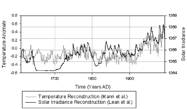
Figure 1: A comparison of the solar irradiance and surface air temperature reconstructions.

We approach the problem of quantifying the sun-climate connection on decadal timescales by examining the correlation between spectral features of solar irradiance and global temperature reconstructions as a function of time. Using the method of wavelet analysis, we can objectively determine the dominant solar forcing frequencies in any given year. We can quantitatively compare the observed period and phase with the corresponding spectral characteristics of the temperature reconstruction. In effect, we can examine the sun-climate correlation as a function of both time and frequency.

While correlation studies between solar irradiance and climate variables have been done before [Crowley and Kim, 1996; Friis-Christensen and Lassen, 1991; Hoyt and Schatten, 1997; McCormack and Hood, 1996], this study offers several new benefits. Wavelets allow us to determine, in any given year, what frequencies present in the solar reconstruction are also present in the temperature data. For example, in 1976 we detect the presence of an 11.54 year solar cycle in the irradiance record; we find the same cycle evident in the temperature record with a phase lag of a few years.

Determining the correlation between the spectral content of two signals offers advantages over comparing directly the raw time signals: the wavelet transform acts as a filter, allowing us to examine frequencies of interest while excluding much of the stochastic variability and background noise inherent in the original signal. Furthermore, reliable techniques exist for establishing the statistical validity of the results [Torrence and Compo, 1998]. By applying wavelet transforms to these signals, we are able to analyze both the frequency content of each signal, and also the time dependence of that content.

We compute wavelet transforms of the solar and temperature reconstructions, and compare them using two different schemes: the Pearson’s correlation method and the conditional probability method. In this paper we focus on timescales of the (approximately) 11-year solar cycle. The results of our analysis show that a nonzero correlation between solar irradiance and terrestrial temperature on this timescale requires a phase lag between the two data sets; this is not surprising since we expect terrestrial response to lag behind solar output. Hence we study the correlation between wavelet transforms of solar output in one year with wavelet transforms of terrestrial temperature an arbitrary number of years later. We search for the optimal phase lag that maximizes the correlation. By choosing an appropriate phase shift for each year, we do find a significant, positive sun-climate correlation for most of the period AD 1720-1950.

Because the solar cycle length varies in time, we improve our results further by identifying the appropriate solar-cycle length as a function of time, again using wavelets. Then we compute the irradiance-temperature wavelet spectra correlation at the corrected timescale. We find that the phase-optimized correlations oscillate in time. In the case of the sun-climate correlation corrected for phase lag and solar cycle length, we find that the strength of the correlation is not at all constant in time: in fact, the correlation increases and decreases between 0.12 and 0.71 (in a range between -1 and 1) over several intervals throughout the past 400 years. We find that the phase lag varies from 0-10 years.

We present also a test for the possible role of stochastic resonance in the sun-climate system. Stochastic resonance is a mechanism whereby a weak, periodic signal is amplified by the noise associated with a nonlinear system with more than one minimum. We suggest here a test to determine whether terrestrial response to solar output is enhanced via stochastic resonance.

Many authors have addressed the issue of solar climate forcing, including: [Andronova and Schlesinger, 2000; Reid, 2000; van Loon and Labitzke, 2000; Rind, Lean, and Healy, 1999; Karl and Trenberth,1999; Mann, Bradley, and Hughes, 1998; North and Stevens, 1998; White, et al., 1997]. General circulation models (GCMs) provide an alternative approach to investigate solar climate forcing by simulating climate dynamics [Andronova and Schlesinger, 2000; Rind, Lean, and Healy, 1999; Marshall, et al. 1994]. This paper presents work complementary to such efforts by investigating directly the relationship between reconstructed sun and climate data sets.

In Section II we discuss the paleoclimate reconstructions that we use. In Section III we review the basic theory of wavelet analysis, and then obtain wavelet transforms of both the solar irradiance and the surface air temperature data sets. In Section IV, we use two different methods to obtain wavelet correlations between the solar irradiance and terrestrial temperature data sets, in order to compare the 11-year wavelet transforms. We use the Pearson’s method as well as the conditional probabilities method. In Section V we discuss the results of our study. We introduce in Section VI a proposal for using wavelets to extract information about the existence of stochastic resonance in the data. We conclude in section VII with a summary of our results.

This paper deals with the sun-climate connection on decadal timescales, focusing on the approximately 11-year solar cycle. Future work will investigate the solar-climate connection on longer timescales of centuries to millenia, with the goal of addressing the solar vs. anthropogenic contributions to increasing terrestrial temperatures.

2 Paleoclimate Reconstructions

Since we are interested in assessing the sun-climate connection on decadal time scales, we need robust solar and climate indicators extending back hundreds of years. Reliable global temperature records exist for only the past century, and measurements of solar irradiance have only been made for twenty years. To work beyond the limitations of instrumental records, we must turn to paleoclimate reconstructions.

2.1 Solar Activity

The intensity of radiation from the sun reaching the surface of the earth, currently about $1365$ W/m², is subject to cyclic behavior on several time scales. The most prominent of these variations are the well known 11-year solar cycle and its 22-year sub-harmonic or Hale cycle, and evidence also exists for longer term variability, particularly the 88-year Gleissberg cycle [Hoyt and Schatten, 1997; Schatten, 1988]. In addition, millennial-scale solar variability is present as a result of changes in the earth’s orbit [Berger, 1991]. As a measure of decadal and centennial-scale solar variability, we use the total solar irradiance reconstruction of Lean, Beer, and Bradley [1995].

Extending back to AD 1610, the reconstruction is based on a number of proxy measurements including historical sunspot records and cosmogenic isotope abundance measurements. The upper panel of figure 4 shows this mean annual solar irradiance as a function of time. Several interesting features are evident in the reconstruction– most notably the period of depressed solar output from 1650-1710, the Maunder minimum. The reconstruction also exhibits an upward trend, particularly in the twentieth century.

2.2 Climate Activity

We adopt as our indicators of climate the multi-proxy surface air temperature (SAT) reconstructions of Mann et al., and Jones et al. [Mann, Bradley, and Hughes 1998; Jones, et al., 1998]. We utilize these temperature reconstructions (rather than using other climate indicators such as annual precipitation or cloud cover) because temperature is by far the most extensive and reliably reconstructed global data set. Using a network of widely distributed proxy climate indicators, Mann et al., and Jones et al., have reconstructed the mean Northern Hemisphere surface temperatures over a time period extending back to AD 1000. The global network of indicators includes dendroclimatic, ice core, ice melt, coral, and extensive instrumental records. Reconstructions from individual sites are spatially averaged to obtain a Northern Hemisphere mean. Using global reconstructions attenuates the significant overprint by ocean and atmospheric circulation expected in regional climate records on the timescales of interest. Figure 2 shows the Northern hemisphere surface temperature reconstructions of Mann, et al., and Jones, et al. (The two time series reconstructions are not identical; however, differences in phase and amplitude may be caused by seasonal and spatial sampling in the reconstructions [Mann, et al. 2001]). Both plots are characterized by a gentle cooling that ends abruptly with a dramatic 20th century warming trend.

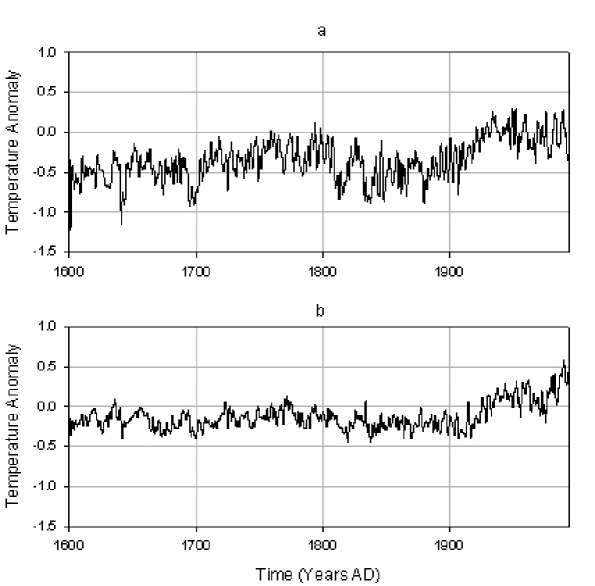
Figure 2: Northern hemisphere surface air temperature anomaly (in ^∘C) reconstructions of a) Jones, et al. [1998], and b) Mann, Bradley, and Hughes [1998].

3 Wavelet Analysis

The basic goal of wavelet analysis is to both determine the frequency content of a time series, and assess how that frequency content changes in time. This stands in contrast to conventional Fourier analysis that allows one to determine what frequencies appear in the signal, but fails to efficiently reveal the time dependence of those spectral features. When signals are fraught with localized, high frequency events, or when phenomena exist on diverse timescales and at different times, the wavelet transform is the tool of choice. In recent years, wavelets have found an increasing number of applications in geophysical and astrophysical research. For example, Weinberg, Drayson, and Freese have used wavelet analysis to examine the formation and development of abnormally low total ozone events [1996]. Others have used wavelets to specifically examine solar variability. Willson and Mordinov have used wavelets to establish sunpots and faculae as primary causes of total solar irradiance variability [Willson and Mardinov, 1999]. Continuous wavelet transforms have also been used by Fligge, Solanki, and Beer to assess the time dependence of the solar cycle length [Fligge, Solanki, and Beer, 1999], by Frick, et al. to analyze stellar chromospheric activity variations [Frick, et al., 1997], and by Weng and Lau to determine variability of satellite radiance measurements [Weng and Lau, 1994].

3.1 Basic Theory

One can expand a complex time signal as the sum of certain basis functions– in the case of Fourier analysis, these basis functions are sines and cosines of different frequencies. Because these functions are perfectly localized in frequency, it is straightforward to determine what frequencies are present in the original signal; on the other hand, because the functions are not at all localized in time, it is quite difficult to find where in time those frequencies happen to be. Wavelet analysis circumvents this problem by expanding a time signal in terms of a set of basis functions localized in both time and frequency domains. Each of these “wavelets” is a function of two parameters: the dilation parameter, $a$, which determines the scale or frequency of the wavelet function; and the translation parameter, $b$, which determines the time at which the function is centered. A wavelet family is generated from a single analyzing, or mother wavelet by these translations and dilations,

$${\psi_{ab}=\frac{1}{\sqrt{a}}\psi\left(\frac{t-b}{a}\right)}$$ (1)

The function $\psi(t)$ must fulfill several conditions in order to be considered a wavelet. First, it must satisfy the admissibility, or zero mean condition,

$${\int^{+\infty}_{-\infty}\psi(t)dt=0}$$ (2)

Secondly, its localization in both time and frequency domains must satisfy the following criterion: its spread in time, $\delta t$, and frequency, $\delta\omega$, must satisfy an uncertainty principle, $\delta t\delta\omega\geq\mbox{const.}$

The wavelet transform $w_{ab}$ of a signal $f(t)$ is a convolution of the signal with the wavelet basis functions, and hence depends on the translation and dilation parameters,

$${w_{ab}=\int^{\infty}_{-\infty}f(t)\psi\left(\frac{t-b}{a}\right)dt}$$ (3)

We often consider the normalized wavelet power spectrum,

$${P_{ab}=\frac{|w_{ab}|^{2}}{\sigma^{2}}},$$ (4)

where $\sigma$ is the variance of the original time series.

There are a number of popular choices for the mother wavelet function that are well suited to probing geophysical signals. In this work, we use the second derivative of a Gaussian, the so-called “Mexican-hat” function,

$${\psi(t)=c(1-t^{2})\mbox{e}^{-t^{2}/2},}$$ (5)

where the constant factor, $c=\sqrt{4/3\sqrt{\pi}}$, ensures that the wavelet function at each scale has unit energy (i.e. $\int\psi^{2}_{ab}(t)dt=1$).

In the appendix we address two important technical issues: edge effects and statistical significance. The preceding analysis works well as long as we are not interested in spectral features near the boundary of our signal. Near the beginning and end of finite time series, however, we need to modify the wavelet basis functions to avoid spurious results. To attenuate these edge effects, our analysis is performed using the adaptive wavelets discussed in Appendix A. Using the methods developed by Frick, et al., we allow our wavelet basis functions to “adapt” their shape based on the presence or absence of data in the time series [1997].

Furthermore, in order to discern between essential physical features of the geophysical signals and those background noise processes that may mimic them, we must have a means of assessing the statistical significance of our wavelet transform. Our approach to this issue is detailed in Appendix B.

As a concrete demonstration of the value of wavelets, consider figure 3. The figure depicts a signal consisting of two sine waves of two different frequencies that are distinctly separated in time. A conventional Fourier analysis would reveal two peaks, one corresponding to each frequency, but would offer no information as to where in time those frequencies dominate. The wavelet transform, shown in the lower portion of the figure, shows not only the two different frequencies, but also discloses when each frequency dominates.

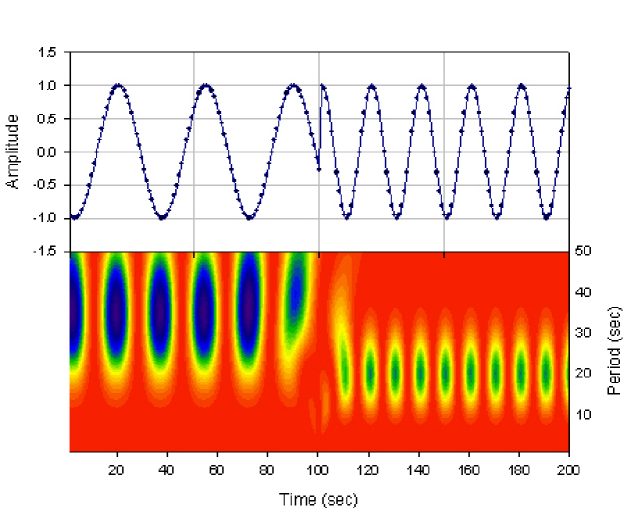
Figure 3: Upper panel: a time signal containing two distinct frequencies. Lower panel: a density plot representing the wavelet transform of the time signal. From 0 to 100 seconds, the time signal (upper panel) has a period of 35 seconds, and the wavelet transform exhibits distinct peaks corresponding to a period of 35 seconds during this interval. After 100 seconds, the period of the time signal decreases to 20 seconds and this abrupt change is clearly reflected in the plot of the wavelet transform.

3.2 Wavelet Transform of Solar Irradiance

The first step in assessing the sun-climate link is to apply the wavelet transform to each of the solar and climate reconstructions. Figure 4 plots both the solar irradiance reconstruction of Lean et al., and its corresponding wavelet power spectrum. Significant peaks with a period near 11-years are evident in the wavelet power spectrum, indicating the presence of the well-known solar cycle throughout the last several centuries; however, the solar cycle is notably absent during the Maunder minimum, which stretches from roughly 1650-1710 [Baliunas, et al., 1999].

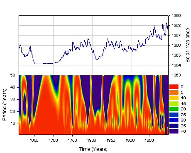
Figure 4: Upper panel: the total solar irradiance as reconstructed by Lean, Beer, and Bradley [1995]. Lower panel: the wavelet transform of the solar irradiance, calculated using the Mexican hat wavelet of Eq. 5.

Although traditionally considered to be 11-years, the length of the solar cycle actually changes in time [Ochadlick and Kritikos, 1993; Fligge, Solanki, and Beer, 1999]. To objectively determine the frequency content of the solar wavelet transform, we look for peaks in the wavelet power spectrum $P_{ab}$ corresponding to periods between three and twenty years. To ensure that the peaks are real, i.e. not a result of background noise, we use the statistical significance tests outlined in Appendix A. We require that the value of $P_{ab}$ at $(a,b)$ exceed the expected red noise background (as given by Eq. 14) at the 95% confidence level. We find over the past four centuries, that 35 years exhibit significant power within this range. Following Fligge, et al., we chart in figure 5 the solar cycle length as a function of time [Fligge, Solanki, and Beer, 1999]. The mean solar cycle length obtained by this method is $10.93\pm 1.53$ years (statistical error).

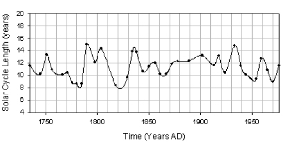
Figure 5: Solar cycle length as a function of time, as determined from the wavelet power spectrum of the solar irradiance reconstruction of Lean, Beer, Bradley [1995].

3.3 Wavelet Transform of Surface Air Temperature

A similar analysis may be made of the mean annual northern hemisphere global surface air temperature (SAT) reconstructions. Figure 6 plots the SAT reconstruction from Mann, Bradley, and Hughes [1998] along with its wavelet power spectrum.

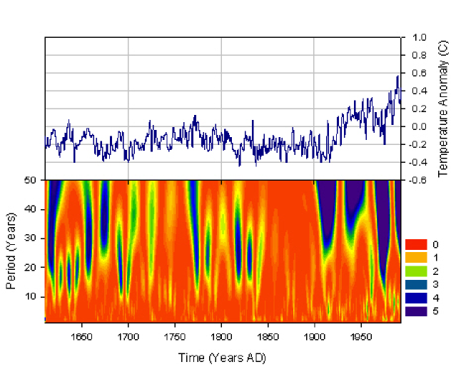
Figure 6: Upper Panel: the surface air temperature as reconstructed by Mann, Bradley, and Hughes [1998]. Lower panel: the wavelet transform of the temperature calculated using the Mexican hat wavelet of Eq. 5.

4 Wavelet Correlation

4.1 Comparison of 11-Year Wavelet Transforms

We may directly compare the 11-year components of the solar and temperature wavelet transforms. Figure 7 plots horizontal slices through the wavelet transforms of figures 4 and 6 at the 11-year wavelet period. In the solar irradiance wavelet transform, the periodic presence of a strong 11-year cycle throughout the past few centuries is readily apparent, except during the Maunder minimum. On the other hand, the 11-year cycle is continuously apparent in the Mann temperature record. The next step in assessing solar-climate forcing is to quantitatively determine correlations between solar and temperature wavelet transforms, i.e. between horizontal slices such as those depicted in figure 7, taken at the appropriate timescales. Because the length of the solar-cycle varies somewhat in time, we obtain correlations both for the 11-year timescales, and also those as determined in figure 5.

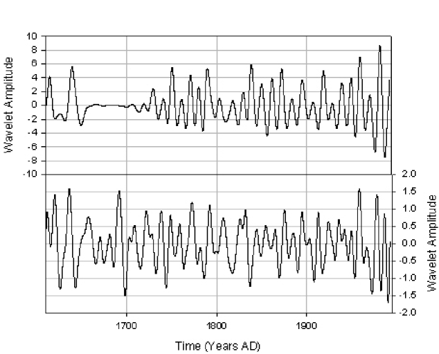
Figure 7: Upper panel: the eleven year components of the solar irradiance wavelet transform. Lower panel: the eleven year components of the surface air temperature reconstruction of Mann, Bradley, and Hughes [1998].

4.2 Methods of Correlation

Once the frequency content of the solar and climate reconstructions has been established using wavelet analysis, the next step is to determine how closely the spectral features of one time series correlate with those of another. To do this we will compare the spectra using two independent techniques.

4.2.1 Pearson’s Method

The first of these methods is based on Pearson’s correlation coefficient, which measures the linear correlation between two time series. That is, for two time series $x(t)$ and $y(t)$, the correlation between them is given by,

$${\rho(\phi)=\frac{\sum_{t}(x(t-\phi)-\bar{x})(y(t)-\bar{y})}{\sqrt{\sum_{t}(x(t-\phi)-\bar{x})^{2}\sum(y(t)-\bar{y})^{2}}}}$$ (6)

where $\bar{x}$ represents the mean of the time series $x(t)$. Here, $\rho=\pm 1$ indicates a perfect positive or negative correlation. We have written the correlation as a function of $\phi$, the phase lag between the two time series. Since terrestrial climate does not instantly respond to solar fluctuations, the solar irradiance and temperature records will not necessarily be in phase; in fact, recent models suggest that surface temperatures can lag irradiance by up to ten years [Rind, Lean, and Healy, 1999]. By displacing the time series records with respect to each other by an amount $\phi$, we can measure the correlation as a function of phase lag.

Furthermore, we have no reason to expect the influence of the sun on the climate to remain constant in time; in fact, we would like to be able to track changes in the sun-climate correlation from year to year. To do this, we measure the correlation between subsets of our time series defined by a window of width $N$, centered at a time $t_{0}$. In the results that follow, we take $N=50$ years. Within the range $50\leq N/{\rm years}\leq 100$ we have verified that the results do not depend sensitively on the window width; smaller window widths offer increased time resolution at the expense of statistical significance. By varying $t_{0}$, we slide the window along the time series to obtain a time resolved measure of correlation.

4.2.2 Conditional Probability Method

The second correlation method is based on conditional probabilities. This method has the advantage that is does not depend upon any assumption of a linear relationship between the two time series. Given two time series, $x(t)$, and $y(t)$, we consider the following conditional probability,

$${P(\phi)=[x(t-\phi)\geq\alpha|y(t)\geq\beta];}$$ (7)

that is, the probability that $x(t-\phi)$ is greater than constant $\alpha$, given that $y(t)$ exceeds some other constant $\beta$. The constant values $\alpha$ and $\beta$ are typically chosen to be the mean of the time series under investigation. A large probability implies that when one signal exhibits a large amplitude, the other signal does also. Since $P(\phi)$ is a probability, it may take values between 0 and 1, with zero indicating little correlation, and 1 indicating a high degree of correlation. This method, as with Pearson’s, may accommodate a phase lag $\phi$; similarly, we can also achieve time resolution using a sliding window of fixed width. The conditional probability method requires no assumptions about the linear relationship between signals, and numerical experiments indicate that the method is a reliable measure of how closely two time series track each other.

5 Results

We determine the correlation between the wavelet power spectra of the solar irradiance reconstruction of figure 4 and the surface air temperature reconstruction of figure 6. We will begin by comparing the 11-year components of the solar and temperature wavelet power spectra, which have been plotted in figure 7. First, we will compute correlations for the case where the irradiance and temperature wavelet spectra are in phase; this case would correspond to an instantaneous response of the temperature to changes in the irradiance. After this simplest case, we will generalize our results in two ways: 1) we will consider the possibility of a phase lag between solar variation and climate response, and 2) because the solar cycle length is not constant in time, we compute the correlation between wavelet components of different periods. In particular, we will find the correlation for the appropriate solar cycle length, as plotted in figure 5. For simplicity of presentation, we will focus in this section primarily on a comparison of Lean solar irradiance and Mann temperature reconstructions. However, we have in fact performed identical calculations using the Jones temperature reconstruction as well; the results will be compared at the end.

5.1 Comparison of 11-Year Wavelet Power with Zero Phase Shift

To quantitatively compare the 11-year components of the two wavelet spectra shown in figure 7, we use the Pearson’s method to measure the correlation as a function of time. In figure 8, the correlation is plotted as a function of time with zero phase lag, i.e., $\phi=0$. The dashed lines indicate the 95% confidence level for the correlation; that is, the correlation is only significant outside of these lines. We see that, for most of the data set, the correlation is statistically insignificant. Additionally, the correlation is both positive and negative. A positive correlation indicates that an increase in power in the irradiance wavelet spectrum corresponds to an increase in power in the temperature wavelet spectrum. A negative correlation indicates that an increase in irradiance wavelet power is met with a decrease in temperature wavelet power.

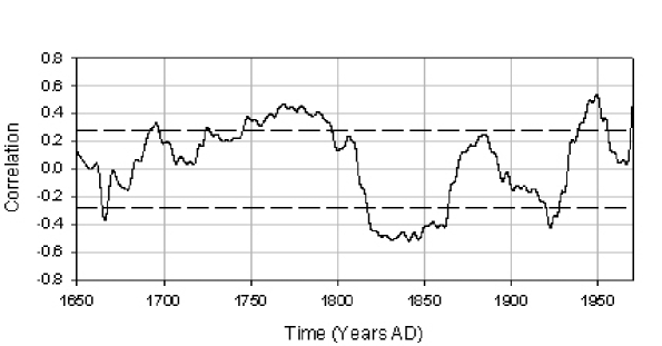
Figure 8: The correlation between the 11-year components of solar irradiance and temperature (Mann et al. data) wavelet spectra as a function of time (measured with respect to the solar irradiance record), for zero phase shift between the signals. The dashed lines indicate the 95% confidence level for the correlation; that is, the correlation is only significant outside of these lines. For most of the data set, the correlation is statistically insignificant. Correlation has been obtained using Pearson’s method.

However, we do not believe this plot is an accurate characterization of sun-climate correlation for several reasons. First, we do not expect the earth’s climate to respond instantaneously to solar variations. There undoubtedly exists a phase lag between irradiance and temperature; furthermore, the phase lag may vary in time. Allowing for phase lags radically changes the results. This first modification is the most important one. Second, although of less significance, is our exclusive use of the 11-year components in the above plot. In fact, we know that the length of the solar cycle varies in time. We can improve our assessment of solar climate forcing by using the appropriate solar cycle length, as calculated above and plotted in figure 5.

5.2 Comparison of 11-Year Wavelet Power with Optimal Phase Shift

To demonstrate the sensitivity of our results to the more important of the two effects, the phase lag, we compute the correlation between irradiance and temperature wavelet spectra as a function of both phase lag and time, still for the 11-year components. The result is plotted in figure 9.

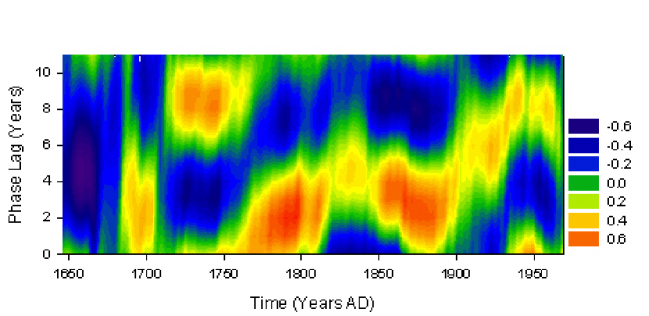
Figure 9: The correlation between wavelet power spectra of the irradiance reconstruction and the surface air temperature reconstruction (Mann et al.) at the 11-year wavelet period. The correlation is plotted as a function of both phase shift and time. The strength of the correlation is color coded in the range (-1,1), from strong negative to strong positive correlation. Time is plotted for the solar irradiance wavelet spectrum, and phase lag is relative to this time. Correlation has been obtained using Pearson’s method.

Figure 8 is the horizontal slice at the bottom of figure 9. Whereas the correlation in figure 8 becomes negative over several intervals, figure 9 demonstrates that one can always find a positive correlation by choosing an appropriate phase shift. For each year, one can find the phase shift that yields the maximum correlation; this amounts to following the yellow-red ridge in the plot. Because we do not a priori know the correct phase shift between the sun and the climate in a given year, we adopt as an “optimal” phase shift that shift that yields the maximum correlation. We require the optimal phase shift to lie in the range $0\leq\phi\leq 10$ years; we choose $\phi\geq 0$ because a positive phase shift corresponds to terrestrial temperature changes lagging behind solar irradiance variations, rather than the other way around. For the remainder of this paper, we will always use this optimal phase shift.

Figure 10 plots this maximum correlation as a function of time, still for the 11-year components. Again, the dashed-line indicates the 95% confidence level above which the correlation is statistically significant. No statistically significant negative correlations exist now, but strong, significant positive correlations clearly stand out. In fact, the correlations are statistically significant throughout most of the range 1720-1955, i.e., after the Maunder minimum and until the recent past.

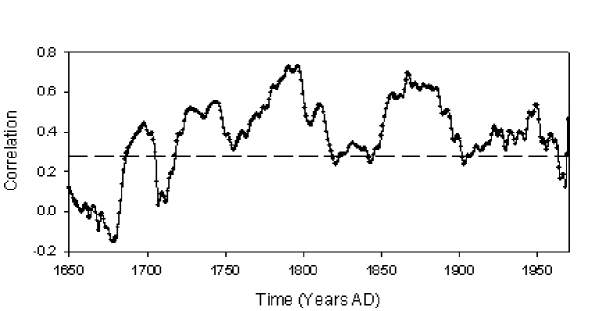
Figure 10: The maximum correlation between wavelet power spectra of the irradiance reconstruction and the surface air temperature reconstruction (Mann et al.) at the 11-year wavelet period. Here, the phase lag between solar output and terrestrial response has been allowed to vary so as to maximize the correlation. Time is plotted appropriate to the solar irradiance wavelet spectrum. The dashed line indicates the 95% confidence level above which the correlation is statistically significant. Correlation is computed using the Pearson’s method.

During the period prior to 1700, the lack of significant correlations at any phase lag may be due to the presence of the Maunder minimum. We do not examine temperature and irradiance directly, but rather their wavelet power spectra; during the Maunder minimum, no power near the 11-year period exists in the solar record.

5.3 Comparison of wavelet power spectra with appropriate solar cycle length and optimal phase shift

Because the solar cycle length changes in time, we can further improve our assessment of solar-climate forcing. Instead of using an 11-year solar cycle, we now use the corrected solar cycle length plotted in figure 5. We compute correlations between the irradiance and temperature wavelet spectra at the timescale corresponding to the corrected solar cycle length; we continue to use the optimal phase shift (i.e., the one that maximizes the correlation). For example, in the year 1798 we observe a solar cycle length of 12.11 years in the solar irradiance reconstruction. We calculate the correlation between the 12.11-year components of the irradiance and temperature wavelet power spectra at the optimal phase shift, which in 1798 is 3 years. We can make such a calculation for each of the 35 years for which we obtained a solar cycle length in figure 5. Figure 11 plots both the maximum correlation and optimal phase shift for each of these years.

In figure 11, we see the time dependence of the optimal phase lag throughout the 400 years of the data sets. Note the large variability of this phase lag, with values ranging from 0 to 10 years. Of course we may wonder about the veracity of very high (e.g. 10 year) phase lags. Early on in the data, we find a large phase lag is required; the phase lag dips to be quite small for about 150 years, and around 1900 begins to rise again.

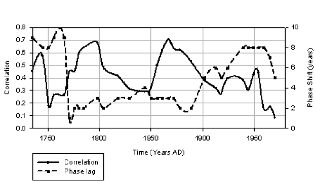
Figure 11: The solid line tracks the correlation for each of the 35 years for which we obtained a solar cycle length in figure 5; the solid line shows the maximized correlation between the wavelet power spectra of the surface air temperature reconstructions of Mann et al. and the solar irradiance reconstruction. The dotted line tracks the optimal phase shift, i.e., the phase shift necessary to achieve maximum correlation. Time is appropriate to the solar irradiance spectrum. Correlation has been computed using the Pearson’s method.

All of the results we have presented in this section have used only the Mann et al. surface air temperature reconstruction, but we have also performed the same analysis with the Jones et al. SAT reconstruction. For comparison, the maximum correlations of both the Mann et al. and Jones et al. are plotted together in figure 12.

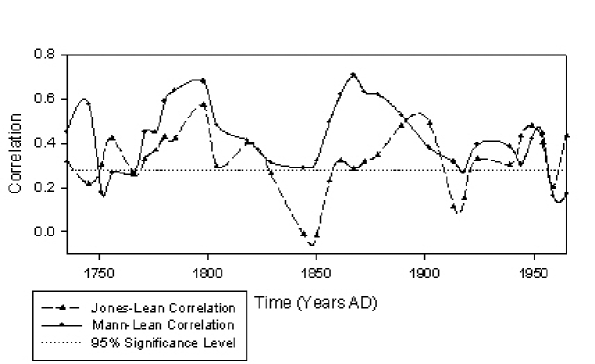
Figure 12: The solid line plots the maximum correlation between wavelet spectra of solar irradiance and the surface air temperature reconstructions of Mann et al.. The dashed line plots the same correlation for the temperature reconstruction of Jones et al. The straight dotted line represents the 95% confidence level above which correlations are statistically significant. Time is appropriate to the solar irradiance spectrum. Correlation has been computed using the Pearson’s method.

5.4 Comparison of wavelet spectra for a variety of timescales (with optimal phase shift)

The focus of this paper is the solar cycle timescale of roughly 11 years. However, the wavelet transforms that we have obtained to date of the solar irradiance and temperature data have yielded much additional information, on scales from 1-50 years. Hence we can investigate the sun-climate correlation on all of these timescales simultaneously by plotting the maximum correlation as a function of time and wavelet period. The results are shown in figure 13. As before, we allow $0\leq\phi\leq 10$ years. In future work we will explore even longer timescales of centuries to millenia with these wavelet techniques.

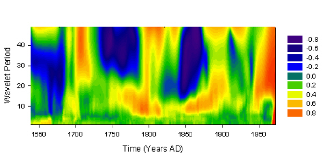
Figure 13: Maximum correlation between solar irradiance and temperature (Mann et al) wavelet spectra, as a function of both time (appropriate to the solar irradiance reconstruction) and wavelet period. Correlation has been computed using Pearson’s method.

5.5 Results using the Probability correlation method

The preceding analyses have all utilized the Pearson’s correlation method. In addition, we have performed the same calculations with the probability correlation method, as a check on our results. Figure 14 compares the results of applying Pearson’s correlation method with that obtained by applying the probability method. In both cases, we compute the correlation between the wavelet power spectra of the Mann, et al. SAT reconstruction, and the Lean, et al., solar irradiance reconstruction, adjusted for optimal phase shift and the appropriate solar cycle length. Although the two measures of correlation are not identical, both contain similar features as a function of time. Since the probability correlation method does not depend on a linear relationship between the two time series, it is encouraging that both methods give the same results.

5.6 Phase Lags

Several authors have previously addressed the phase relationship between solar forcing and climate response. Their results differ markedly from ours. We believe our wavelet analysis to be superior to any previous work on this subject. Thomson claimed moderate, in-phase coherence between Northern Hemisphere global temperatures and sunspot records from 1854 to 1923; from 1923-1991 the same records suggest temperatures 180^∘ out of phase with the solar cycle [Thomson, 1995]. Analyzing the same data, Lawrence and Ruzmaikin reported very different results: they claimed a negative coupling with a phase shift of $\phi\approx-135^{\circ}$ (i.e., with temperature changes leading solar changes) during the period 1860-1920, switching abruptly to a positive coupling ($\phi\approx 45^{\circ}$) from 1920 to the present [Lawrence and Ruzmaikin, 1998]. Furthermore, studies by Currie indicate a possible geographic dependence of the solar-climate phase [Currie, 1993]. Examining United States temperature records, Currie finds that cyclic temperature variations are in phase with solar irradiance East of the Rocky Mountains, while west of the Rockies they are 180^∘ out of phase.

Our work instead uses wavelet analysis to determine an optimal phase lag. This approach has many advantages. By using wavelet transforms of the data we are able to obtain information exclusively on the timescales of interest, namely the solar cycle timescale; the timescale itself is obtained using wavelets (see figure 5). Using wavelets we are clearly able to identify the power on solar cycle timescales at different times, and are able to compare the power in the solar irradiance and terrestrial temperature data. The results of our study are plotted in figure 11. Roughly, we see that temperature records lag solar irradiance records by roughly 90^∘ from 1760 to 1878, then become nearly 180^∘ out of phase until 1924; from 1924-1970, the phase lag is nearly 270^∘. Note that our study only uses global mean averages of the annual data; we have not studied geographic variations.

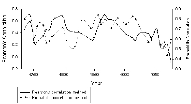
Figure 14: The solid line represents the Pearson’s correlation between the wavelet power of the surface air temperature reconstruction of Mann et al. and the solar irradiance reconstruction. The dashed line tracks the correlation between the same power spectra using the probability correlation method, using the same optimal phase shifts. Time is plotted appropriate to the solar irradiance reconstruction.

6 Stochastic resonance in solar climate forcing: speculation

The results of the previous sections reveal the presence of a time dependent correlation between the terrestrial temperature and solar irradiance, but do not provide a mechanism by which this sun-climate correlation may vary. In fact, the means by which apparently insignificant variations in the incident solar radiation seem to effect relatively large changes in the Earth’s temperature remains an outstanding problem of climate science. The phenomenon of stochastic resonance has been proposed as a mechanism for enhancing the effects of weak forcings[Benzi, et al., 1982]. In particular, a weak periodic forcing signal is amplified by the noise associated with a nonlinear system [Gammaitoni, et al., 1998; McNamara and Wiesenfeld, 1989; Bulsara and Gammaitoni, 1996]. Lawrence and Ruzmaikin have recently proposed that the phenomenon of stochastic resonance may be an important factor in the solar forcing of the climate on 11-year timescales [Lawrence and Ruzmaikin, 1998]. We here illustrate a method (using wavelet techniques) that allows us to test whether or not stochastic resonance has helped to drive solar climate forcing.

Stochastic resonance is a mechanism whereby a weak, periodic forcing signal is amplified by the noise associated with a nonlinear system with more than one minimum. The classic example of stochastic resonance involves an overdamped particle moving in a noisy, quartic potential well,

$${U(x)=-\frac{a}{2}x^{2}+\frac{b}{4}x^{4}}$$ (8)

where $a$ and $b$ are constants that depend on the nature of the problem. The minima for the potential are located at $x=\pm\sqrt{a/b}$, and the height of the potential barrier is $a^{2}/4b$.

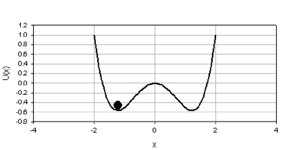
Figure 15: A bistable, quartic potential.

The potential is plotted in figure 15 for a=1.5 and b=1. The particle naturally resides in one of the two stable minima, but an external forcing signal may provide the energy necessary for the particle to move over the potential barrier and down into the adjacent minima. In a noiseless system, if the external forcing signal is too weak, the particle will always remain in one of the minima; however, in a noisy system, the particle may exploit some of the noise energy to leap from minimum to minimum, in phase with the weak forcing signal. In a sense, the weak signal cooperates with the noise to induce a relatively large change in the system.

Lawrence and Ruzmaikin propose that under certain conditions, terrestrial climate systems exhibit a bistability that allows stochastic resonance to amplify a weak 11-year solar signal, thereby producing “transient correlations” between the sun and the terrestrial climate. Whether an appropriate bistability exists in the climate system is unclear, but Ruzmaikin suggested that the ENSO oscillations may act as a stochastic driver, exciting transitions between normal atmospheric states and anomalous ones such as the Pacific North American (PNA) pattern [Ruzmaikin, 1999].

To test whether the observed, transient correlations of figure 11 could be induced by stochastic resonance (regardless of the physical nature of the bistability), we look for a “hallmark” feature of stochastic resonance: the response of the system to a driving signal depends on the intensity of the noise in the system. It is a general feature of stochastic resonance models that the response of the system peaks at a particular value of the noise intensity.

For a bistable system, such as the quartic potential discussed above, one can show that, under certain circumstances, the dependence of response on noise at the fundamental forcing frequency is,

$${\mbox{response}\propto\left(\frac{Ac}{D}\right)^{2}\exp(-U_{\mbox{max}}/D)}$$ (9)

where $A$ is the amplitude of the driving signal, $c$ is the separation of the minima, $U_{\mbox{max}}$ is the height of the potential barrier, and D is the intensity of the noise in the system. This dependence is plotted in figure 16. Although details of the signal response curve depend on the specific system, the fact that response varies with noise intensity is a “fingerprint” feature of stochastic resonance models.

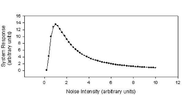
Figure 16: The response, as a function of noise intensity, of a bistable nonlinear system driven with a weak, periodic signal. The peak indicates stochastic resonance.

To test whether or not the solar climate system exhibits stochastic resonance, we generate an analogous plot from our data and compare it with figure 16. We take the sun-climate correlation (between wavelet power spectra on “the adjusted 11-year” time scale), as plotted in figure 11, as a measure of system response. Our system thus exhibits two states: one corresponding to a high sun-climate correlation, and the other to a small sun-climate correlation. As a crude measure of noise intensity, we use the variance of the original temperature time series reconstruction. In other words, we use the variations in Earth temperature as a measure of the noise inherent to the climate system. We will investigate whether these changes in temperature variance strongly affect the magnitude of the sun-climate correlation.

Because the variance of the temperature record changes in time, we can track its effect on the sun-climate correlation. To obtain a plot analogous to figure 16, we plot the sun-climate correlation in a fifty-year window versus the noise in that window. The result is shown in figure 17.

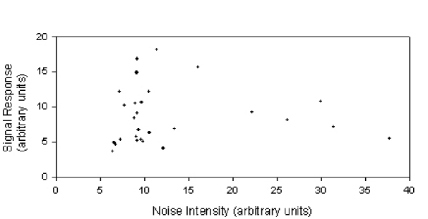
Figure 17: The sun climate correlation as a function of the noise inherent to the system, as estimated by the variance of terrestrial temperature.

The plot suggests that the sun-climate correlation varies as a function of noise intensity, and it even bears a passing resemblance to figure 16. However, we must be cautious: the range of temperature variance is quite small, and most of the points on the plot have a variance between 5 and 15 units. Unfortunately, we are unable to tune the noise as one would in an experiment. We have only a limited terrestrial temperature record to work with. Given this data set, we have no ability to change the intensity of the noise background; we are limited by the natural nonstationarity inherent to the system. Furthermore, we have no reason to believe that a simple bistable potential (such as the one that gives rise to figure 16) adequately represents the terrestrial climate.

There are a number of additional caveats. The use of the variance of the temperature reconstruction as a proxy for noise intensity is most likely naive. The relevant stochastic background may not be noise fluctuations associated with the temperature itself, but rather with some other stochastic phenomenon, such as the ENSO driver, as suggested by Ruzmaikin. Furthermore, assuming that the sun-climate correlation is a good indicator of system response may also be inadequate. Detailed climate models sensitive to stochastic resonance type phenomena may help assess the validity of these ideas.

The transient sun-climate correlation depicted in figures 10 and 11, exhibits a period on the order of 50 years. Because we are examining the sun-climate correlation on 11-year time scales, the presence of such a long period is difficult to explain. Systems exhibiting stochastic resonance are most likely to switch states when the periodic driver peaks; thus, in our case, we would expect the sun-climate correlation to switch from high to low (or vice-versa) on average every, $11/2\approx 5.5$ years. Longer term solar cycles (such as the 88-yr Gleissberg cycle) may force the climate system to switch states on 40-50 year scales, producing the observed transient correlations. Alternatively, because the 11-year forcing signal is so weak, the earth may reside in one state for several (i.e. 4-5) forcing periods before transitioning to the other. In future work we will use wavelets to examine other tests of stochastic resonance in the Earth/Sun system.

Hence our analysis does not exclude stochastic resonance as a possible mechanism by which solar-climate forcing proceeds; in fact, the presence of transient sun-climate correlations and a possible dependence of the sun-climate correlation on background noise intensity suggests that stochastic resonance may be present.

7 Conclusion

We have used wavelet analysis as a tool to investigate the response of terrestrial temperatures to solar variations. Wavelet transforms of solar irradiance and surface air temperature reconstructions are plotted in figures 4 and 6, and reveal the time dependence of the spectral content in those signals. From the wavelet transform of the solar irradiance reconstruction, we objectively determine the solar cycle length as a function of time by looking for peaks in the wavelet spectrum. Using two different methods, we examine the correlation between the wavelet power spectra of the irradiance and temperature records. In this paper we have focused on solar-cycle timescales (near 11 years). In future work, we will extend the analysis to include centennial and millennial-scale variations.

Determining the correlation between the spectral content of two signals is more robust than comparing directly the raw time signals: the wavelet transform acts as a filter, allowing us to examine frequencies of interest while excluding much of the stochastic variability and background noise inherent in the original signal. In addition, we can assess the strength of the correlation on individual timescales, and track that correlation as a function of time.

We have computed the correlation as a function of both phase $\phi$ and time t, where $\phi$ is the phase shift between the solar irradiance and terrestrial temperature wavelet power spectra (i.e., in some sense, the phase lag between solar forcing and climate response).

7.1 Summary of Results

First, we studied the 11-year components of the solar irradiance and surface air temperature wavelet power spectra. We found that, for $\phi=0$ (no phase shift between the signals), there is almost no statistically significant correlation between these components, as shown in figure 8. This result is not surprising, because we expect that the earth takes some time to respond to changes in the sun. A time dependent phase shift must be introduced to obtain a positive correlation of any significance.

Next, we allowed for phase shifts between the solar irradiance and terrestrial temperature wavelet spectra. We looked for the optimal phase shift, i.e., that phase shift that maximizes the correlation. We plotted the correlation as a function of phase lag and time for the 11-year components in figure 9. By choosing an appropriate phase for each year (following the yellow-red ridge in figure 9), we observe that it is possible to achieve a positive correlation. Indeed, we found a significant, positive sun-climate correlation for most of the period AD 1720-1950 (i.e. after the Maunder minimum and until the recent past). This result is plotted for the 11-year timescale in figure 10.

Because the solar cycle length varies in time, we improved our results further by finding the appropriate solar-cycle length, as plotted in figure 5, and computing the irradiance-temperature wavelet spectra correlation at that timescale. This correlation is presented in figures 11 and 12. One can see that the phase-optimized correlations of figures 10, 11, and 12 oscillate in time.

In the case of the sun-climate correlation corrected for phase lag and solar cycle length, shown in figure 11, we found that the strength of the correlation is not at all constant in time: in fact, the correlation increases and decreases between 0.12 and 0.71 over several intervals throughout the past 400 years. One could speculate that there exists some periodicity in the strength of the earth’s response to solar irradiance. The time dependence of the phase lag between earth and sun that would give the maximum correlation between the two signals is plotted over the 400 years of the data set in Figure 13.

Additionally, we plotted the correlation between the irradiance and temperature for wavelet period from 1-50 years, for the optimal phase shift in the range $0<\phi<10$ years. We also speculated on the role of stochastic resonance in this variability in the sun-climate system and presented a possible test for this effect.

Appendix A Wavelet Analysis: Edge Effects

When we are interested in spectral features near the boundary of our time series, we must consider edge effects. Near the beginning and end of a finite time series, the wavelet function becomes unable to satisfy the admissibility condition of Eq. 2, leading to spurious modifications of the wavelet transform in the vicinity of the boundaries. To attenuate these edge effects, our analysis is performed using adaptive wavelets. Using the methods developed by Frick, et al., we allow our wavelet basis functions to “adapt” their shape based on the presence or absence of data in the time series [1997].

We consider a time series, $f(t)$, that is defined over some finite time interval, and which may contain a finite number of “gaps”, where no data has been recorded. To keep track of observed data, we define a gap function, $G(t)$, that is equal to one everywhere data is present and zero otherwise. Using this approach, the boundaries are thus viewed as semi-infinite gaps in the signal. We replace our wavelet $\psi(t)$ with a modified analyzing wavelet, $\psi^{\prime}(t)$.

$${\psi^{\prime}(\frac{t-b}{a})=\psi(\frac{t-b}{a})G(t)}$$ (10)

Near a gap, this modified wavelet “breaks”, becoming unable to satisfy the admissibility condition of Eq. 2. In this manner we shift the blame from the incomplete data set $f(t)$, to an improperly constructed wavelet function $\psi^{\prime}(t)$.

To fix the problem we replace $\psi^{\prime}$ with an adaptive wavelet, $\tilde{\psi}$, which changes shape to guarantee that the admissibility condition is always satisfied. We accomplish this by writing our analyzing wavelet as the product of two functions,

$${\psi=h(t)\Phi(t)}.$$ (11)

In the case of the Mexican hat wavelet used in this analysis, $\Phi(t)$ is the positive definite Gaussian function, exp$(-t^{2}/2),$ and $h(t)$ represents the modulating parabola $c(1-2t^{2})$. The adaptive wavelet is then defined as,

$$\tilde{\psi}(t,b,a)=\left[h\left(\frac{t-b}{a}\right)-C(a,t)\right]\Phi\left(\frac{t-b}{a}\right)G(t).$$ (12)

The function $C(a,t)$ is determined by requiring that $\int\tilde{\psi}(t)dt=0$

$$C(a,t)=\left[\int_{-\infty}^{\infty}\Phi\left(\frac{t-b}{a}\right)G(t)dt\right]^{-1}\times\\ \int_{-\infty}^{\infty}h\left(\frac{t-b}{a}\right)\Phi\left(\frac{t-b}{a}\right)G(t)dt.$$

The gap function must be determined specifically for each data set. In practice, the reconstructed time series are padded with zeros, with the gap function specifying the limits of the actual data. This technique reduces but does not eliminate the error; one must still be wary of spectral features that fall near the boundaries of the time series. Our results will not rely on those portions of the wavelet transform strongly affected by residual edge effects.

Appendix B Wavelet Analysis: Background noise and statistical significance

In order to discern between essential physical features of the geophysical signals and those background noise processes that may mimic them, we must have a means of assessing the statistical significance of our wavelet transform. Wavelet statistical significance tests are accomplished by comparing the normalized wavelet power spectrum $P_{ab}$ with the expected noise power spectrum $P_{noise}$. Thus, in order to judge statistical significance, we must first understand the background noise associated with our signal. Geophysical noise backgrounds are often modeled as either white noise (having a flat Fourier spectrum), or red noise (having more power at lower frequencies).

Following Torrence and Compo, the background noise in the time series reconstructions used in this paper are modeled as first order autoregressive (AR-1) processes, also known as a Markov process [1998]. The simplest model for an AR-1 time series $x_{t}$ is,

$$x_{t}=\alpha x_{t-1}+z_{t},$$ (13)

where $z_{t}$ is normally distributed white noise, and the parameter $\alpha$ is the lag-1 autocorrelation coefficient of the .

It can be shown that the expected Fourier spectrum for an AR-1 noise process is given by,

$$P_{AR-1}(k)=\frac{1-\alpha^{2}}{1+\alpha^{2}-2\alpha\cos(2\pi k/N)}$$ (14)

where $N$ is the number of points in the time series and $k$ is the frequency index. Because the background contains more power at lower frequencies, it is termed a red-noise spectrum. Numerical experiments performed by Torrence and Compo bear out the hypothesis that the spectrum of Eq. (14) is also the expected local wavelet power spectrum at a time $b_{0}$ (i.e., the function $P_{noise}(a)=|w_{a,b=b_{0}}|^{2}$) [1998].

Torrence and Compo also confirm, by Monte Carlo simulation, that the actual noise spectrum is $\chi^{2}$-distributed about the predicted mean background spectrum.  In particular, for real wavelets, such as the Mexican-hat used in this analysis,

$$P_{noise}\rightarrow P_{AR-1}(k)\chi_{1}^{2}$$ (15)

where the arrow indicates “is distributed as”.

The noise background of our signals can be estimated by determining the lag-1 autoregressive coefficient, $\alpha$, appearing in Eq.(13). The coefficient $\alpha$ is estimated from the original geophysical time, $y_{i}$, series by

$$\alpha=\frac{\sum_{i=1}^{i=N}(y_{i}-\bar{y})(y_{i-1}-\bar{y})}{\sum_{i=1}^{i=N}(y_{i}-\bar{y})^{2}}.$$ (16)

By assessing the statistical significance of our results, we may filter those regions of the wavelet spectra associated with stochastic variability and known noise processes, thereby enhancing our ability to detect real signals. Knowing the expected power spectrum and the distribution, we may establish levels of confidence to distinguish a physical component of the wavelet spectrum from the noise background. We regard the wavelet spectrum as significant if it exceeds the expected noise background of Eq. (15) at the 95% confidence level.

References

- [1] Andronova N.G, and M. Schlesinger, Causes of global temperature changes during the 19th and 20th centuries. Geophys. Res. Lett. 27 (14): 2137-2140. Jul 15, 2000.
- [2] Baliunas, S., P. Frick, D. Sokoloff, and W. Soon, Time scales and trends in the central England temperature data (1659-1990): A wavelet analysis, Geophys. Res. Lett., 24, 1351. 1997.
- [3] Benzi, R., G. Parisi, A. Sutera, and A. Vulpiani, Stochastic resonance in climatic change, Tellus 34, 10-16, 1982.
- [4] Berger A. and M.F. Loutre, Insolation values for the climate of the last 10 million years. Quat. Sci. Rev., Vol. 10 No. 4, 297-317, 1991.
- [5] Bulsara, Adi, and Luca Gammaitoni, Tuning In To Noise. Phys. Today, pp.39. March, 1996.
- [6] Burroughs, W.J., Weather Cycles: real or imaginary, Cambridge University Press, Cambridge, 1992.
- [7] Crowley, T.J. and K.-Y. Kim, Towards development of a strategy for determining the origin of decadal-centennial scale climate variability, Quat. Sci. Rev. 12, 375-385, 1993.
- [8] Currie, R. G., 1993, Luni-solar 18.6 and solar cycle 10-11 year signals in USA air temperature records. Intl. J. of Climatology, 13, 31-50.
- [9] Fligge, M., S.K. Solanki, and J. Beer, Determination of solar cycle length variations using the continuous wavelet transform. Astron. Astrophysics. 346, 313-321, 1999.
- [10] Frick, P., S. Baliunas, D. Galyagin, D. Sokoloff, and W. Soon, A Wavelet Analysis of Solar Chromospheric Activity Variations, ApJ. 483, 426-434, 1997.
- [11] Friis-Christensen, E., and K. Lassen, Length of the Solar Cycle: An indicator of solar activity closely associated with climate, Science, 254, 698-700, 1991.
- [12] Gammaitoni, L. Peter Hanggi, Peter Jung, Fabio Marchesoni, Stochastic Resonance. Rev. of Mod. Phys., Vol. 70. 223-287. 1998
- [13] Hoyt, D., and K. Schatten, The Role of the Sun in Climate Change, 279, Oxford University Press, New York, 1997.
- [14] Jones, P.D. K.R. Briffia, T.P. Barnett, and S.F.B. Tett, High-resolution Paleoclimatic Records for the Last Millenium: Interpretation, Integration, and Comparison with General Circulation Model Control-Run Temperatures., The Holocene 8, 455-471. 1998.
- [15] Karl T., and K. Trenberth, The human impact on climate. Sci. Amer. 281 (6): 100-105. Dec, 1999.
- [16] Kumar, Praveen and Efi Foufou-Georgiou, Wavelet Analysis for Geophysical Applications. Rev. of Geophys., 35, 4, 385-4512, 1997.
- [17] Lawrence, J.K., and A.A. Ruzmaikin, Transient solar influence on terrestrial temperature fluctuations. Geophys. Res. Lett. Vol. 25, No. 2, 159-162, 1998.
- [18] Lean, J., J. Beer, and R. Bradley, Reconstruction of solar irradiance since 1610: Implications for climate change. Geophys. Res. Lett., 22, 3195, 1995.
- [19] Mann, Michael, R. Bradley, and M. Hughes, Global-scale temperature patterns and climate forcing over the past six centuries. Nature., 392, 779-787. 1998.
- [20] Mann, Michael, Raymond Bradley, Malcolm Hughes, and Philip D. Jones, Reply to “It Was the Best of Times, It Was the Worst of Times”. Science. 280 (5372). 2001.
- [21] Marshall, S., R. Oglesby, J. Larson, and B. Saltzman, A comparison of GCM sensitivity to changes in CO2 and solar luminosity. Geophys. Res. Lett., 21 (23): 2487-2490 Nov 15, 1994.
- [22] McCormack J., and L. Hood, Apparent solar cycle variations of upper stratospheric ozone and temperature: Latitude and seasonal dependences. J. of Geophys. Res.- Atmos. 101 (D15): 20933-20944. Sep 20, 1996.
- [23] McNamara, B. and K. Wiesenfeld, Theory of Stochastic Resonance, Phys. Rev. A., 39, 4854-4869, 1989.
- [24] North G., and M.J. Stevens, Detecting climate signals in the surface temperature record. J. of Climate, 11 (4): 563-577. Apr, 1998.
- [25] Ochadlick, A. and H. Kritikos, Variations in the Period of the Sunspot Cycle. Geophy. Res. Lett., 20, 1471-1474, 1993.
- [26] Petit, J.R., I. Basile, A. Leruyuet, D. Raynaud, C. Lorius, J. Jouzel, M. Stievenard, V.Y. Lipenkov, N.I. Barkov, B.B. Kudryashov, M. Davis, E. Saltzman, and V. Kotlyakov, Four climate cycles in the Vostok ice core. Nature. 387:359. 1997.
- [27] Pittock, A.B., A critical look at long-term sun-weather relationships, Rev. Geophys. Space Phys., 16 400-420, 1978.
- [28] Reid G.C., Solar variability and the Earth’s climate: Introduction and overview. Space Science Reviews. 94 (1-2): 1-11, Nov 2000.
- [29] Rind, D. J. Lean, and R. Healy, Simulated time-dependent climate response to solar radiative forcing since 1600. J. of Geophys. Res., 104, Number D2, 1973-1990, 1999.
- [30] Rind, D., and J. Overpeck, Hypothesized causes of decade-to-century-scale climate variability- climate model results. Quat. Sci. Rev. 12 (6): 357-374 1993.
- [31] Ruzmaikin, A., Can El Nino amplify the solar forcing of climate? Geophy. Res. Lett. Vol. 26, No. 15. 2255-2258, 1999.
- [32] Schatten, K.H., A model for solar constant secular changes. Geophys. Res. Lett., 15, 121-124, 1988.
- [33] Thomson, David J., The Seasons, Global Temperature, and Precession. Science. Vol 268. April, 1995.
- [34] Torrence, Christopher, and Gilbert P. Compo, A Practical Guide to Wavelet Analysis. Bulletin of the Amer. Meteor. Soc., 79, No. 1 61-78, 1998.
- [35] van Loon H, and K. Labitzke, The influence of the 11-year solar cycle on the stratosphere below 30 km: A review. Space Sci. Rev. 94 (1-2): 259-278. Nov, 2000.
- [36] Weinberg, Beth., Roland Drayson, and Katherine Freese, Wavelet Analysis and Visualization of the formation and evolution of low total ozone events over Northern Sweden. Geophys. Res. Lett., 23, 2223. 1996.
- [37] Weng, H., and K.-M. Lau, Wavelets, period-doubling and time-frequency localization: application to satellite infrared radiance data analysis. J. Atmos. Sci. ,51, 1994 2523 - 2541.
- [38] White W.B., J. Lean, D. Cayan, and M.D. Dettinger, Response of global upper ocean temperature to changing solar irradiance. J. of Geophs. Res. 102 (C2): 3255-3266. Feb 15, 1997.
- [39] Willson, Richard and Alexander V. Mordinov, Time-Frequency Analysis of Total Solar Irradiance Variations. Geophys. Res. Lett., Vol. 26, No. 24, 3605-3608, Dec. 15th, 1999.