SINP MSU 2002-9/693
astro-ph/0203478; v.3

Clusters of EAS with electron number $\mathbf{\gtrsim 10^{4}}$

Abstract

We perform cluster analysis of arrival times of extensive air showers (EAS) registered with the EAS–1000 Prototype array in the period from August, 1997 till February, 1999. We present twenty cluster events each consisting of one or several EAS clusters, study the dynamics of their development, and analyze the angular distribution of EAS in clusters. We find that there may be certain correlation between EAS clusters with mean electron number $\sim 10^{5}$ on the one hand and gamma-ray bursts and ultrahigh energy cosmic rays on the other.

1 Introduction

There are a considerable number of articles devoted to the analysis of arrival times of extensive air showers (EAS) (see, e.g., [1, 2, 3, 4, 5, 6, 7, 8] and references therein). In this paper, we address this problem using the experimental data obtained with the EAS–1000 Prototype array. This array operates at the Skobeltsyn Institute of Nuclear Physics of Moscow State University. It consists of eight detectors situated in the central part of the EAS MSU array along longer sides of the $64\mbox{ m}\times 22$ m rectangle. The array registers EAS generated by cosmic rays with the energy of a primary particle more than $10^{14}$ eV [9, 10].

For the purposes of the present investigation, we selected 203 days of regular operation of the array in the period from August 30, 1997 till February 1, 1999. The total EAS number in this data set equals 1 668 489. The mean interval between consecutive EAS arrival times is equal to 10.5 sec. The discreteness in the moments of EAS registration is approximately 0.055 sec (one tic of the PC clock). Parameters of EAS were found using a program written by V. P. Sulakov [11]. The mean electron number in the EAS under consideration is of the order of $1.2\times 10^{5}$ particles.

As we have mentioned above, this paper is mainly devoted to the analysis of EAS arrival times. Certain results of our investigation have already been presented briefly in [6, 7, 12]. Here we shall go into some details concentrating on EAS clusters.

One may study arrival times either as a sequence of consecutive moments of time $t_{1}$, $t_{2}$,…, $t_{n}$, where $t_{i}$ is the moment of registration of the $i$th EAS, or as a sequence $x_{1}$, $x_{2}$,…, $x_{n}$ of time intervals (“delays”) between consecutive EAS: $x_{i}=t_{i}-t_{i-1}$, $i=1,\dots,n$, where $t_{0}=0$ corresponds to midnight. Since we are interested in EAS clusters, let us discuss their possible formal definitions.

One can define an EAS cluster at least in two different ways:

1. a cluster is a group of consecutive EAS in which all $x_{i}$ are less than some predefined value $\xi$ which in turn is much less than the mean delay $\bar{X}=\frac{1}{n}\sum_{1}^{n}x_{i}$;

2. a cluster is a group of $k$ consecutive EAS such that the full “length” $L_{j,k}=x_{j}+x_{j+1}+\cdots+x_{j+k-1}$ of this group is much less than the expected length that is equal to $k\bar{X}$.

When one uses any of these definitions, a natural question appears: How one should choose $\xi$ or $k$? In general, as soon as the mean delay $\bar{X}$ is known, one has considerable freedom in the choice of $\xi$ or $k$. Actually, if one uses the second definition, then it is possible to select clusters as groups such that $L_{j,k}\leqslant k\bar{X}/a$, $a=2$, $3$, $4$,… But this way makes it difficult to estimate the probability of appearance of the corresponding cluster since the statistical distribution of $x_{i}$ is not known a priori. Thus it seems more reasonable to study the distribution of $x_{i}$ first.

As is well known, the vast majority of statistical methods aimed for time series analysis are developed for stationary time series. Recall that the most common definition of a stationary process found in textbooks (often called strong stationarity) is that all conditional probabilities are constant in time (see, e.g., [13, 14]). Our previous investigation of the distribution of EAS arrival times has revealed that in general case time series obtained during a sufficiently long period of time are not stationary [6, 7]. We have also found that the main reason that makes our time series non-stationary is the barometric effect. Namely, it was found that the mean number of EAS registered in a time unit is inversely proportional to the atmospheric pressure. This dependence can be approximately expressed by a simple formula:

$$\ln N=-\beta P+\mathrm{const},$$

where $N$ is the number of EAS registered in a time unit, $P$ is the atmospheric pressure, mm Hg, and $\beta$ is the barometric coefficient [10, 11]. For the EAS–1000 Prototype array, the value of $\beta$ varies in the interval (1.08–1.24)$\times 10^{-2}$ depending on the concrete data sample and chosen time bin. For our data set, the statistical error in the value of $\beta$ is of the order of $10^{-4}$. It is easy to see that $\beta=1.08\times 10^{-2}$ is the most “pessimistic” for a search of clusters since it gives the highest intensity of EAS registration for a fixed atmospheric pressure.

As we have already shown, almost all samples of sufficient length in our data set are stationary and satisfy the homogeneity hypothesis if we take into account the barometric effect, though certain deviations have been observed for some samples [6, 7]. If one considers homogeneous samples, then it is possible to point out an interval of time delays for which one may accept a hypothesis that time delays have exponential distribution. In other words, for such a set of time delays the number of EAS registered in a unit of time (“the count rate”) obeys the Poisson distribution. This hypothesis has been verified on the basis of $\chi^{2}$–criterion.

On the other hand, it is known that different statistical criteria can lead to different conclusions (see, e.g., [14]). This made us to apply one more criterion to the same data set to verify the above hypothesis. Namely, we have used a criterion that is based on the variable

$$A=\sqrt{\frac{n}{2}}\,\left|\frac{S^{2}/\bar{X}-1}{\bar{X}}\right|,$$

which has standard Gaussian distribution $\mathcal{N}(0,1)$ for $n$ large enough [15]; here $S^{2}=\frac{1}{n}\sum_{1}^{n}(x_{i}-\bar{X})^{2}$. We have calculated $A$ for different values of $\beta$ and found out that the “best fit” is achieved for $\beta=1.16\times 10^{-2}$. For this $\beta$, $A=0.068$ and one may accept the hypothesis that the intensity of EAS registration for data set as a whole obeys the Poisson distribution (the probability $\mathcal{P}(A<0.08)\approx 0.532$, see [16]). At the same time, the “pessimistic” value of the barometric coefficient $\beta\approx 1.08\times 10^{-2}$ also allows one to accept the hypothesis, since $A=0.070$ for this $\beta$. By this reason, in what follows we shall present the results that were obtained with the “pessimistic” barometric coefficient.

2 The Main Results

To guarantee that the time series under consideration is stationary, we have adjusted experimental arrival times to the atmospheric pressure $P^{*}=742$ mm Hg which is close to the average pressure for the whole analyzed data set. This adjustment was made by the following formula:

$$x_{i}=x_{i}^{0}\exp[\,\beta(P^{*}-P_{i})],$$

where $x_{i}^{0}$ is the experimental time delay, and $P_{i}$ is the atmospheric pressure at the $i$th delay, $i=1,2,\dots,n$. The mean delay for $P^{*}$ is equal to 10.4 sec.

Since we have accepted the hypothesis that the distribution of the number of EAS registered in a time unit obeys the Poisson distribution with the intensity $\lambda\approx 5.77$ min^-1, the following algorithm of cluster selection was accepted:

1. Fix some sufficiently small number $\epsilon>0$ and some duration $T$ of the time interval.

2. Basing on the known intensity $\lambda$ of the Poisson process, find $K$ such that the probability to register more than $K$ showers in time $T$ is of the order of $\epsilon$. Recall that this probability is given by the formula

   $$\mathcal{P}(N_{T}>K)=1-\sum_{k=0}^{K}\frac{(\lambda T)^{k}}{k!},$$

   where $N_{T}$ is the number of EAS registered in time $T$.

3. A sequence of EAS that is registered in a period of time less or equal than $T$ and contains more than $K$ showers is selected as a cluster.

We emphasize that the above hypothesis is not important for our results, but only allows us to estimate the probability of appearance of a cluster.

For the given criterion of cluster selection, we performed a search for EAS clusters using GNU Octave [17] running in Mandrake Linux. The search was arranged in the following way. Fix the initial moment of time $t_{0}=0$, add the chosen time interval $T$ to it and count the number $N_{T}$ of EAS registered in time $T$. If $N_{T}>K$, then take the set of EAS that belongs to $T$ as a cluster; otherwise skip it. After this, move the left end of the time interval $T$ to $t_{1}$ (the arrival time of the first shower in the data set) and repeat the analysis. The procedure goes on until the end of the data set. Notice that this procedure does not exclude the appearance of intersecting clusters. This is possible when one cluster belongs to the time interval $[t_{i},t_{i}+T]$, another one belongs to $[t_{j},t_{j}+T]$, and $t_{j}<t_{i}+T$.

One may certainly choose another strategy of cluster search. For example, one can move along the data set by a sequence of steps with a fixed length. But in this case there is a chance to loose a sufficiently dense cluster that is divided between two intervals. One may also spread time intervals $T$ over the time series in a random way. This procedure seems to be accurate, but it needs a considerable amount of computer time to be performed.

Parameters $T$ and $K$ that were used for the selection of EAS clusters are given in Table 1. These values of parameters has lead to the discovery of eighteen cluster events—sequences of EAS that may be identified as clusters. Below we shall also discuss two events that were chosen for $K$ which was less by a unit than the values given in Table 1. We have added them to the list because they demonstrate certain interesting features. Table 1 also contains an expected number of observed clusters

$$N_{\mathrm{exp}}=\frac{1}{T}\times(\mbox{duration of the observation period})\times\mathcal{P}(N_{T}>K).$$

Table 1: Parameters of selection of EAS clusters and the expected number of corresponding clusters in a 203-day period ($N_{\mathrm{exp}}$).

$T$, sec	$K$	$\mathcal{P}(N_{T}>K)$	$N_{\mathrm{exp}}$	$T$, min	$K$	$\mathcal{P}(N_{T}>K)$	$N_{\mathrm{exp}}$
5	7	$4.6\times 10^{-8}$	0.16	2	30	$1.5\times 10^{-6}$	0.22
10	9	$7.8\times 10^{-8}$	0.14	3	39	$2.1\times 10^{-6}$	0.20
15	11	$4.5\times 10^{-8}$	0.05	4	48	$1.8\times 10^{-6}$	0.13
20	12	$1.3\times 10^{-7}$	0.11	5	57	$1.2\times 10^{-6}$	0.07
25	13	$2.6\times 10^{-7}$	0.18	6	65	$1.3\times 10^{-6}$	0.06
30	15	$7.4\times 10^{-8}$	0.04	7	73	$1.3\times 10^{-6}$	0.05
35	16	$1.1\times 10^{-7}$	0.06	8	81	$1.2\times 10^{-6}$	0.04
40	17	$1.4\times 10^{-7}$	0.06	9	89	$1.0\times 10^{-6}$	0.03
45	18	$1.7\times 10^{-7}$	0.07	10	96	$1.5\times 10^{-6}$	0.04
50	19	$1.9\times 10^{-7}$	0.07	11	104	$1.1\times 10^{-6}$	0.03
55	20	$2.0\times 10^{-7}$	0.06	12	111	$1.4\times 10^{-6}$	0.03
60	21	$2.0\times 10^{-7}$	0.06	13	119	$1.0\times 10^{-6}$	0.02
65	22	$2.0\times 10^{-7}$	0.05	14	126	$1.2\times 10^{-6}$	0.03
70	23	$2.0\times 10^{-7}$	0.05	15	133	$1.4\times 10^{-6}$	0.03
75	24	$1.8\times 10^{-7}$	0.04	16	141	$9.6\times 10^{-7}$	0.02
80	25	$1.7\times 10^{-7}$	0.04	17	148	$1.0\times 10^{-6}$	0.02
85	26	$1.6\times 10^{-7}$	0.03	18	155	$1.1\times 10^{-6}$	0.02
90	27	$1.4\times 10^{-7}$	0.03	19	162	$1.1\times 10^{-6}$	0.02
				20	169	$1.2\times 10^{-6}$	0.02

As one can see, in all cases $N_{\mathrm{exp}}\ll 1$, i.e., if we have strictly Poisson distribution of the count rate, we should observe no clusters at all. But this is not the case, since we have found nearly twenty events that contain one or several (partially) intersecting clusters. It is possible to find a number of other EAS clusters if less strong conditions of their selection are used.

For the purposes of this discussion, we have conditionally divided all events into two groups defined as follows:

• Events that consist of a single cluster (see Table 2a).

• Events that contain several clusters (Tables 2b and 2c).

Let us discuss these two types of events consecutively.

2.1 Single Clusters

As one can see from Table 2a, the first group consists of eight events. Clusters in this group have different length: from approximately 5 seconds to more than 4 minutes. Let us briefly discuss these events beginning with the shortest one.

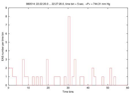
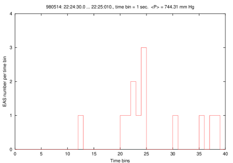
Figure 1: The count rate during an interval that contains a cluster registered on May 14, 1998 (left), see Table 2a, and the “interior structure” of this event (right). In both cases, the cluster begins in the center of the plot. Titles of these and the following figures with the count rate contain the date of the event (yymmdd), the time interval, the time bin, and the average pressure $\langle P\rangle$.

Let us begin with a cluster registered on May 14, 1998 (it was selected for $T=5$ sec). The count rate at an interval that contains this cluster is shown in Fig. 1. Notice that the amplitude of the peak that presents the cluster is nearly 19 times higher than the average value. Remark that though the cluster is very short, the distribution of arrival times of EAS that form this cluster is not uniform. The right plot in Fig. 1 demonstrates that the highest count rate is at the end of this event.

Table 2a: Single clusters. See the parameters of selection in Table 1. Notation: $P$—the atmospheric pressure; $T_{\mathrm{real}}$—the real duration of a cluster (for single clusters), sec; $N_{\mathrm{EAS}}$—the number of EAS in a cluster (group of clusters); $N_{\mathrm{cl}}$—the number of clusters in a group; $T_{\mathrm{adj}}$—the duration of a cluster adjusted to $P^{*}=742$ mm Hg; $\mathcal{P}_{\mathrm{adj}}$—the probability that $N_{\mathrm{EAS}}$ are registered in time $T_{\mathrm{adj}}$. For events marked by $*$ in the $T$-column, $K$ is less by a unit than the value given in Table 1. Moscow local time $T_{M}$ is used: $T_{M}=T_{\mathrm{UT}}+3+\Delta$ (hours); $T_{\mathrm{UT}}$ is the UT time, and $\Delta=1$ hour during Daylight Saving Time, 0 otherwise.

Date	$P$,	$T$,	Beginning	End	$T_{\mathrm{real}}$,	$N_{\mathrm{EAS}}$	$N_{\mathrm{cl}}$	$T_{\mathrm{adj}}$,	$\mathcal{P}_{\mathrm{adj}}$
dd.mm.yy	mm Hg	sec	hh:mm:ss	hh:mm:ss	sec			sec
14.05.98	744.3	5	22:24:50.09	22:24:54.70	4.61	8	1	4.49	$1.9\times 10^{-8}$
24.08.98	735.4	10	07:09:23.89	07:09:33.07	9.17	10	1	9.86	$6.2\times 10^{-8}$
24.12.98	750.5	10	04:29:21.91	04:29:30.64	8.73	10	1	7.97	$8.9\times 10^{-9}$
06.01.99(a)	735.1	25	13:51:57.23	13:52:19.64	22.41	14	1	24.16	$1.5\times 10^{-7}$
28.12.98	740.8	45∗	15:22:33.18	15:23:17.34	44.16	18	1	44.74	$5.4\times 10^{-7}$
05.10.97	717.0	180	20:38:00.60	20:40:17.75	137.15	40	1	179.90	$1.2\times 10^{-6}$
03.01.99	748.6	180	15:36:06.89	15:39:19.73	192.84	40	1	179.49	$1.2\times 10^{-6}$
16.08.98	744.0	240	02:09:42.38	02:13:46.58	244.19	49	1	239.07	$8.8\times 10^{-7}$

Now let us consider longer clusters.

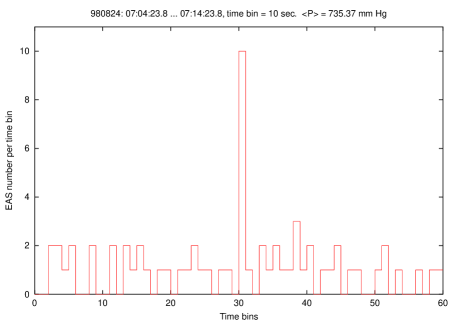
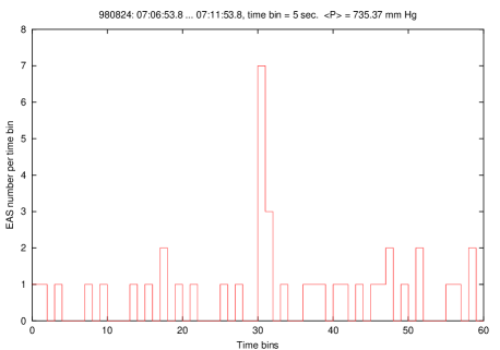
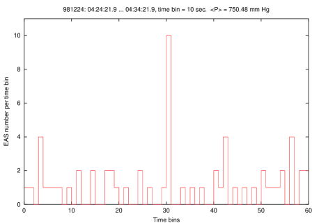
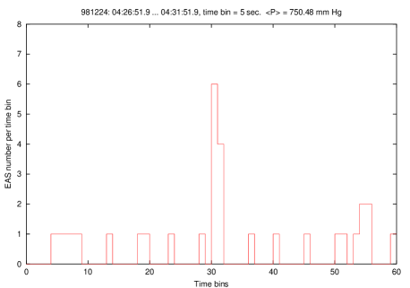
Figure 2: The count rate during time intervals that contain clusters registered on August 24, 1998 (top row) and December 24, 1998 (bottom row), see Table 2a. The right column shows the 5-second structure of the events.

• 24.08.98 and 24.12.98: Both clusters were chosen for $T=10$ sec. They have close duration, consist of an equal number of EAS, and have a very small probability of appearance. The distribution of arrival times of EAS in these clusters is qualitatively the same: the highest count rate is observed at the first half of the events, though the amplitude of the highest peaks is different, see Fig. 2. It is interesting to notice that if we slightly weaken the criterion of cluster search by taking $K=6$ instead of $K=7$ for $T=5$ sec, we find a shorter cluster inside the cluster selected on 24.08.98. For this cluster, 7 showers arrive in 4.06 sec with $T_{\mathrm{adj}}=4.37$ sec and $\mathcal{P}_{\mathrm{adj}}=3.0\times 10^{-7}$.

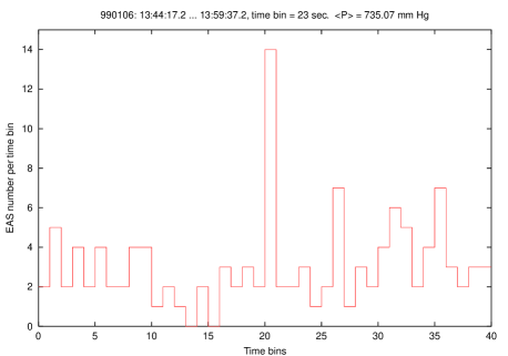
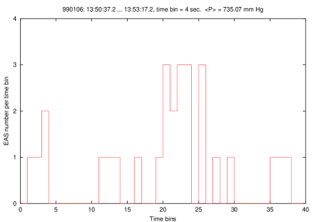
Figure 3: The count rate during time intervals that contain a cluster registered on January 6, 1999(a), see Table 2a. The right plot shows the 4-second structure of the event (bins No. 21–26).

• 06.01.99(a): This cluster is approximately two times longer than two previous clusters, see Table 2a and Fig. 3. It has an interesting “interior structure” if we look at it using 4-second bins. Namely, one can see a “hole” near the end of the cluster: there is a 4-second time interval, during which no EAS have arrived. We shall see below that such “holes” are quite usual for sufficiently long clusters.

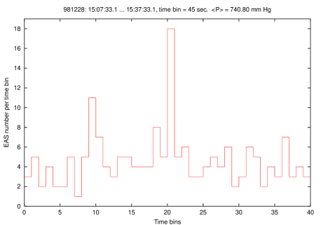
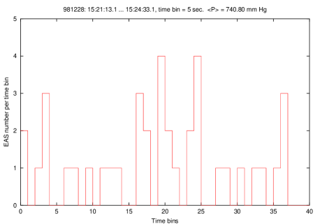
Figure 4: The count rate at an interval that contains a cluster registered on December 28, 1998, see Table 2a. The right plot shows the 5-second structure of the cluster (bins No. 17–25).

• 28.12.98: This event was chosen for $T=45$ sec with $K=17$ instead of $K=18$, see Table 1. We have added it to the list of events because of its possible correlation with some other astrophysical events, see Sec. 4. The cluster has an interesting “interior structure” if one considers 5-second time bins: there are two bins with zero count rate and two bins of equally high count rate equal to 4 EAS per 5 sec, see Fig. 4.

While it is obvious that our selection procedure could not lead to a discovery of a cluster embedded into a 5-second cluster, it may be a bit surprising that clusters which cover several minutes do not contain any shorter clusters inside (compare events registered on 05.10.97, 16.08.98, and 03.01.99 with those presented in Tables 2b and 2c). A natural question arises: Do arrival times of EAS that form these clusters have the uniform distribution? Our analysis reveals that the answer is negative.

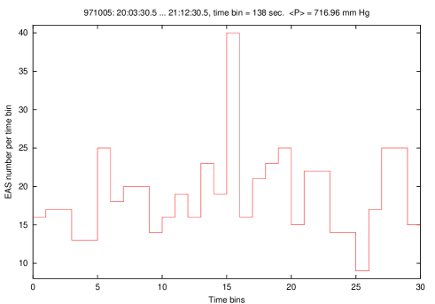
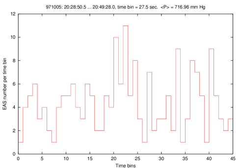
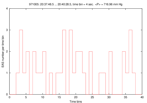
Figure 5: The count rate during time intervals that contain a cluster registered on October 5, 1997, see Table 2a. Two bottom plots reveal the “interior structure” of the cluster. In the middle plot, the cluster occupies bins No. 21–25.

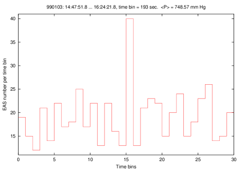
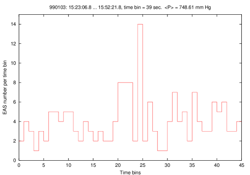
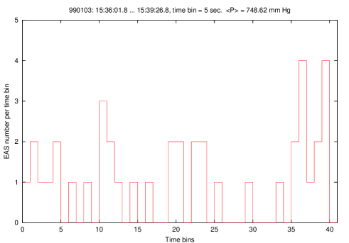
Figure 6: The count rate during time intervals that contain a cluster registered on January 3, 1999, see Table 2a. Two bottom plots reveal the “interior structure” of the cluster. In the middle plot, the cluster occupies bins No. 21–25.

Let us take a look at Figs. 5, 6, and 7. These figures depict the structure of the events registered on October 5, 1997, January 3, 1999, and August 16, 1998 respectively. It is clearly seen that for all three events one can point out short time intervals within a cluster where the count rate is the highest. Let us consider these events in more details:

• 05.10.97 and 03.01.99: Both events were selected for $T=3$ min, see Table 1. They contain equal number of showers, but have different $T_{\mathrm{real}}$ because of different atmospheric pressure at the moments of registration. It is clearly seen from the plots that for these two events, distributions of EAS arrival times are drastically different. For the first cluster, the distribution of EAS arrival times is highly non-uniform, and the highest count rate is observed in the middle and at the beginning of the event (see Fig. 5). For the second cluster, the situation is opposite: the highest count rate takes place at the end of the event (see Fig. 6). Both clusters contain high “sub-peaks,” but none of them is high enough to be selected as a separate cluster.

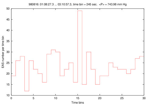
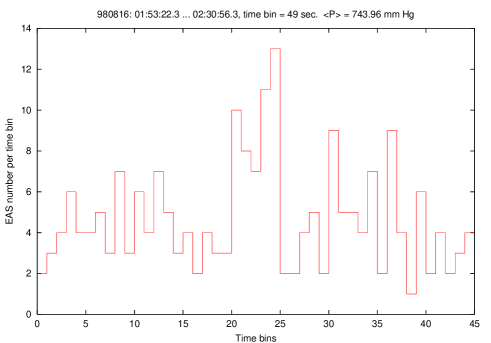
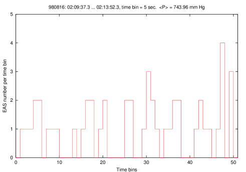
Figure 7: The count rate during time intervals that contain a cluster registered on August 16, 1998, see Table 2a. Two bottom plots reveal the “interior structure” of the cluster. In the middle plot, the cluster occupies bins No. 21–25.

• 16.08.98: This cluster is the longest among single ones. The count rate for this cluster is shown in Fig. 7. It is clearly seen that similar to the above two events, this cluster consists of a number of short bursts, though none of them is intensive enough to form a separate cluster. Fig. 7 also demonstrates that the highest count rate for this event takes place in the end of the cluster.

Thus the arrival times of EAS that form a cluster can have different distributions. More than this, single clusters are not single “bursts” of the count rate with the uniform distribution of EAS arrival times, but consist of several “sub-bursts.” Hence the reason that we find single clusters is that the amplitude of “sub-bursts” is not high enough to satisfy our selection criterion. This is true for all events in the first group.

2.2 Embedded Clusters

Now let us turn to the second group of events. As one can see from Tables 2b and 2c, this group consists of twelve events. It is convenient to divide this group into two subgroups in accordance with the complexity of the events:

1. Simple embedding, see Table 2b.

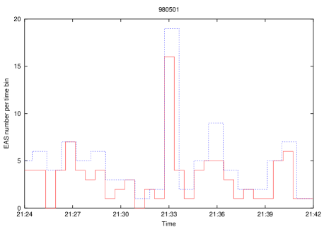
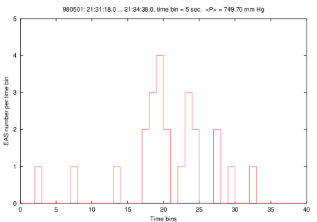
Figure 8: An event registered on May 1, 1998, see Table 2b. The left plot: the innermost cluster (37-second bins) embedded into the outer cluster (55-second bins). The right plot: the 5-second “substructure” of the event (the outer cluster occupies bins No. 18–28).

• 01.05.98: For this event, two clusters are strictly embedded into the longest one. Notice that all clusters begin simultaneously. Fig. 8 shows the innermost and the outer clusters and the 5-second substructure of this event. It is clearly seen how a short cluster appears inside a longer one.

  Notice that this event was selected for the values of $K$ that are less by a unit than those given in Table 1. We have included this event in the list because of an interesting property of the arrival directions of EAS in it, see the discussion in Sec. 3.

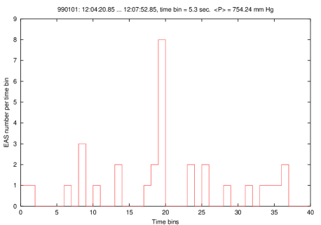
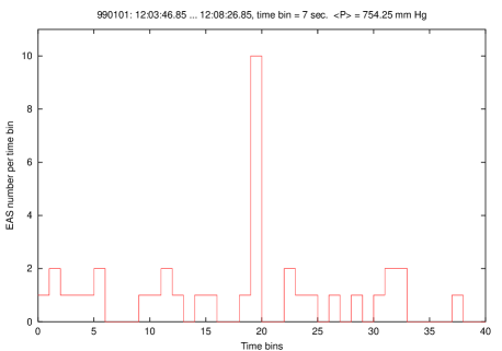
Figure 9: An event registered on January 1, 1999, see Table 2b. The left plot: the interior cluster. The right plot: the outer cluster. In both cases, the cluster ends at the center of the plot.

• 01.01.99: This event is similar to the above one except that it consists of only two clusters, which do not begin, but end simultaneously. It is clearly seen in Fig. 9 that the highest count rate is at the end of the event. Notice that the outer cluster has an extremely small $\mathcal{P}_{\mathrm{adj}}$.

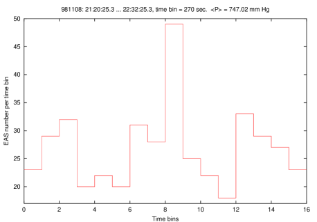
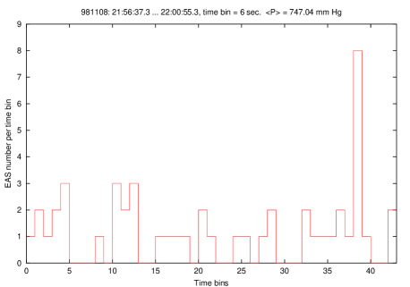
Figure 10: An event registered on November 8, 1998: the outer cluster (left) and its “interior structure” (right). Notice a short cluster (39th bin in the right plot) embedded into the outer one, see Table 2b.

• 08.11.98: An interesting situation takes place for this event, since a 5-second cluster is embedded into a 4-minute cluster, and no clusters of intermediate duration are found, see Fig. 10.

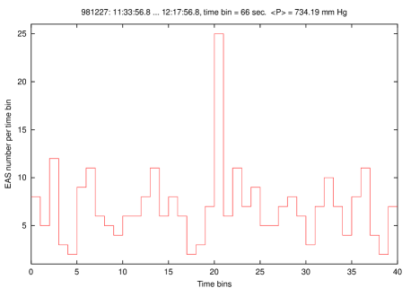
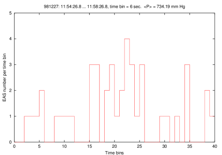
Figure 11: An event registered on December 27, 1998 (left), see Table 2b, and its “substructure” (right). In the latter case, the cluster occupies bins No. 16–26.

• 27.12.98: Two clusters that begin at consecutive showers are selected for $T=70$ sec. We assume that there is no phenomenological reason in the appearance of these two clusters, since they cover exactly the same interval of time as a cluster selected for $T=75$ sec. It is likely that a “real” cluster is the outer one, and thus this event may be referred to the first group. This cluster and its “substructure” are shown in Fig. 11.

Table 2b: Events that consist of several EAS clusters. See notation in Tables 1 and 2a.

Date	$P$,	$T$,	Beginning	End	$T_{\mathrm{real}}$,	$N_{\mathrm{EAS}}$	$N_{\mathrm{cl}}$	$T_{\mathrm{adj}}$,	$\mathcal{P}_{\mathrm{adj}}$
dd.mm.yy	mm Hg	sec	hh:mm:ss	hh:mm:ss	sec			sec
01.05.98	749.7	35∗	21:32:43.01	21:33:19.92	36.91	16	1	33.95	$3.0\times 10^{-7}$
		40∗	21:32:43.01	21:33:21.78	38.77	17	1	35.67	$1.1\times 10^{-7}$
		50∗	21:32:43.01	21:33:37.17	54.16	19	1	49.82	$5.8\times 10^{-7}$
01.01.99	754.2	5	12:06:01.57	12:06:06.84	5.27	8	1	4.62	$2.4\times 10^{-8}$
		10	12:05:59.98	12:06:06.84	6.86	10	1	6.01	$6.4\times 10^{-10}$
08.11.98	747.0	5	22:00:25.36	22:00:30.58	5.22	8	1	4.94	$4.0\times 10^{-8}$
		240	21:56:41.54	22:00:54.63	253.09	49	1	239.65	$9.4\times 10^{-7}$
27.12.98	734.2	70	11:55:56.85	11:57:02.59		25	2
		75	11:55:56.85	11:57:02.59	65.74	25	1	71.55	$5.7\times 10^{-8}$
04.11.98	730.9	30	08:17:44.90	08:18:10.99	26.09	16	1	29.41	$4.7\times 10^{-8}$
		35	08:17:38.91	08:18:09.83	30.92	17	1	34.85	$8.3\times 10^{-8}$
		40	08:17:36.88	08:18:10.99		19	2
		45	08:17:36.88	08:18:10.99	34.11	19	1	38.45	$1.3\times 10^{-8}$
		50	08:17:36.88	08:18:19.56	42.68	20	1	48.10	$8.1\times 10^{-8}$
10.08.98	732.3	50	16:47:43.15	16:48:28.13	44.98	20	1	49.98	$1.5\times 10^{-7}$
		240	16:47:36.61	16:51:19.83		53	5
11.11.98	752.3	900	01:21:17.47	01:38:02.27		136	3
06.01.99(b)	733.2	180	09:22:52.51	09:25:50.41		43	4
08.01.99(a)	726.9	120	03:56:45.66	03:58:28.26		33	3
		180	03:55:50.40	03:58:28.26		44	5
		240	03:55:05.31	03:58:28.26		50	2

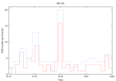
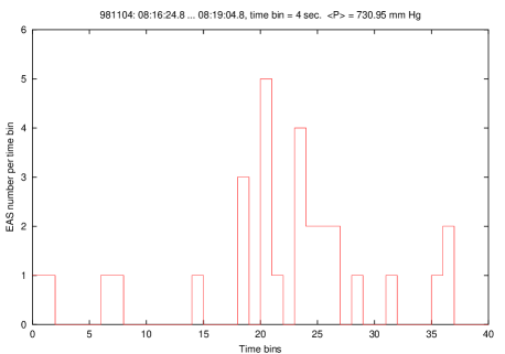
Figure 12: An event registered on November 4, 1998: the innermost (27-second bins) and the outer (43-second bins) clusters (left), see Table 2b, and the 4-second “substructure” of the event (right). In the latter case, the outer cluster occupies bins No. 19–29, the interior cluster occupies bins No. 21–27.

• 04.11.98: For this event, shorter clusters are almost exactly embedded into longer ones. Similar to the event registered on 27.12.98, two clusters selected for $T=40$ sec begin at consecutive EAS and cover exactly the same time interval as a cluster selected for $T=45$ sec. The innermost cluster points at the interval of the highest count rate, see Fig. 12.

  This event has another interesting feature, see the discussion in Sec. 3.

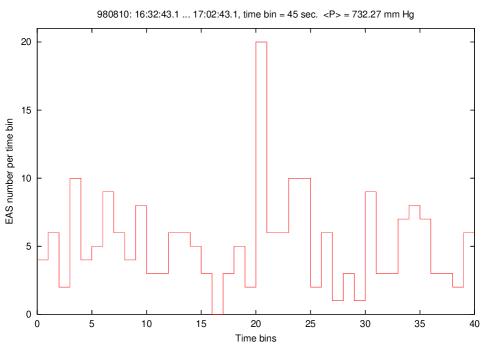
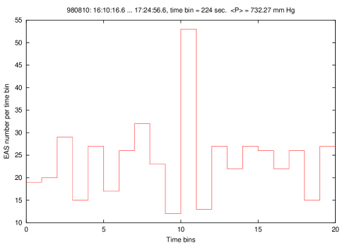
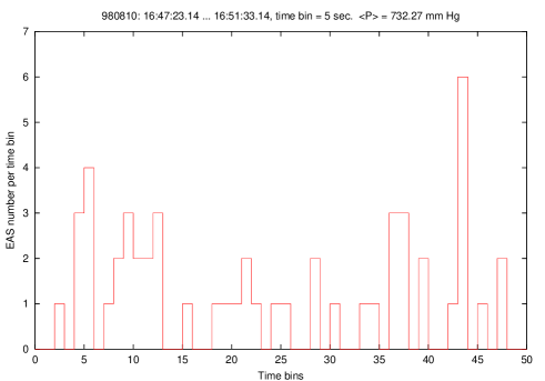
Figure 13: An event registered on August 10, 1998, see Table 2b. From top: the interior cluster, the group selected for $T=240$ sec, and the 5-second “substructure” of the event. In the later case, the interior cluster occupies bins No. 5–13.

• 10.08.98: For this event, a bit more surprising situation takes place: a 45-second cluster is found within a sequence of five nearly 4-minute clusters that begin at consecutive arrival times. The situation is in a sense similar to that one with the event registered on 08.11.98. Notice that the short cluster and the sequence of long clusters begin nearly simultaneously. This event and its “interior structure” are shown in Fig. 13.

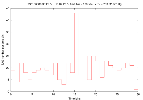
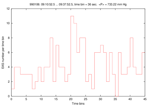
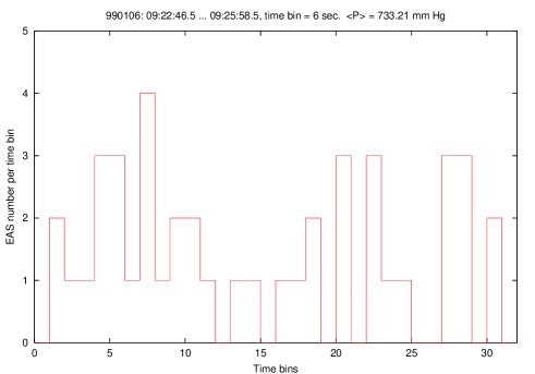
Figure 14: An event registered on January 6, 1999(b) (top plot), see Table 2b, and its “substructure.” In the middle plot, the cluster occupies bins No. 21–25.

• 11.11.98 and 06.01.99(b): For these events, a surprising situation takes place, since a sequence of long clusters (3 and 4 respectively) is found, and no other clusters are inside or outside. All clusters in these events begin at consecutive EAS, and thus it is likely that the only reason of such a situation is a comparatively big time step in $T$ equal to one minute. As one can see from Figs. 14 and 15, it is possible to find intervals of the maximum count rate for these events, too. Namely, the highest count rate is shifted to the beginning of the event registered on January 6, 1999, while for the other event one can find two 20-second bins with maximum count rate, located at the very beginning and soon after the middle of the event respectively.

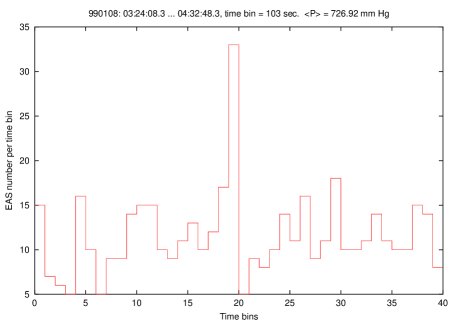
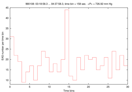
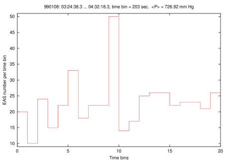
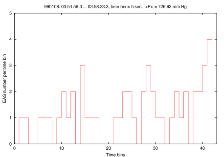
Figure 16: An event registered on January 8, 1999(a), see Table 2b. The embedding of clusters and the “substructure” of the event are shown. Except for the right bottom plot, the clusters end in the center of the plots.

• 08.01.99(a): An event that is similar to the two previous events, but three groups of clusters are found. Each group consists of clusters that begin at consecutive arrival times. The most likely reason of the fact that we do not find a separate cluster neither inside nor outside those given in Table 2b is again the discreteness of $T$. Notice that all sequences end at the same moment of time, and the highest count rate is shifted to the second half of the event, see Fig. 16. It is also interesting to mention that the first group of clusters (selected for $T=2$ min) is almost exactly two times shorter than the third group (selected for $T=4$ min).

2. Complicated embedding, see Tables 2c and 3.

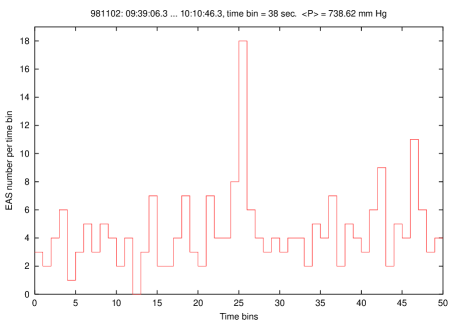
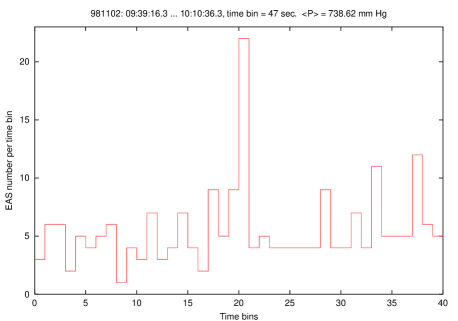
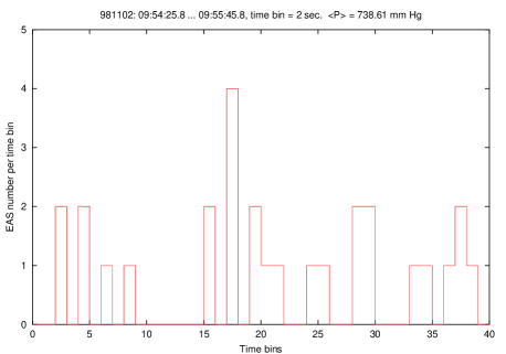
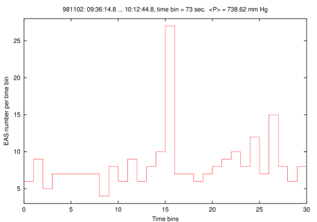
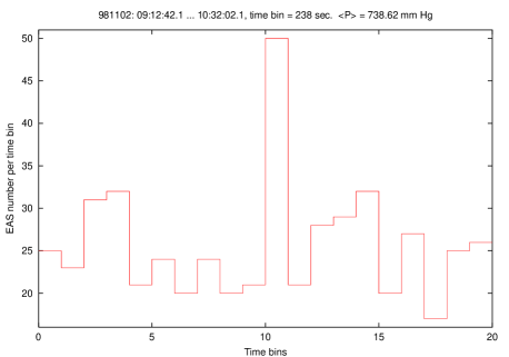
Figure 17: An event registered on November 2, 1998, see Tables 2c and 3. Top row: a cluster selected for $T=40$ sec (left), the first of the clusters selected for $T=50$, 55 sec (right). Middle row: two clusters found for $T=60$ sec (left) (56-second bins are used for the first cluster, 47-second bins are used for the second cluster); the “interior structure” of this group (right): the first cluster occupies bins No. 3–30, the second cluster occupies bins No. 16–39. Bottom row: one of the clusters selected for $T=80$ sec (left): it consists of the showers that form two clusters found for $T=60$ sec, see the text; the outer group of clusters (right).

• 02.11.98: First of all, there is a single cluster found for $T=40$ sec, see the top left plot in Fig. 17. Next, for $T=45,50$, and $55$ sec there are sequences of 4, 3, and 2 consecutive clusters, which begin simultaneously with the 40-second cluster. All three sequences cover the same range of EAS and contain the 40-second cluster. It is remarkable that the first of the clusters selected for $T=50$ and $55$ sec coincide and cover the complete range of EAS arrival times, containing the following clusters inside. Thus this one is the most pronounced of the clusters. It has very small $\mathcal{P}_{\mathrm{adj}}=4.0\times 10^{-9}$: 22 showers arrive in 46.58 sec with $T_{\mathrm{adj}}=48.32$ sec, see the top right plot in Fig. 17.

  For $T=60$ sec, the situation changes: there are two clusters, but to the contrary to the above sequences, they do not begin at consecutive arrival times. The first cluster consists of 22 showers arriving in 55.75 sec ($T_{\mathrm{adj}}=57.84$ sec, $\mathcal{P}_{\mathrm{adj}}=8.4\times 10^{-8}$). The second cluster appears 26.4 seconds later and is more intensive: it also contains 22 EAS, but they arrive in 46.58 sec ($T_{\mathrm{adj}}=48.32$ sec, $\mathcal{P}_{\mathrm{adj}}=4.0\times 10^{-9}$), see Fig. 17, the middle row.

  Next, for $T=65\dots 90$ sec the range of EAS becomes a bit wider. It is interesting that for $T=80$ sec there appears a cluster that covers EAS No. 3717–3744 thus containing the 60-second group (28 showers), see the left bottom plot in Fig. 17. For this cluster, $T_{\mathrm{real}}=72.99$ sec, $T_{\mathrm{adj}}=75.73$ sec, and $\mathcal{P}_{\mathrm{adj}}=3.1\times 10^{-9}$. The same cluster is identified for $T=85$ sec. This makes us conclude that two “shifted” clusters found for $T=60$ sec do not present different astrophysical events but are two “bursts” within one event.

  Finally, for $T=2$, 3, and 4 min the range of EAS covered by clusters becomes more wide, though the right end shifts very little: the first event in $T=4$ min group begins 124.12 sec earlier than the 40-second cluster, but ends only 45.75 sec later, see Table 2c. Thus the highest count rate for this event is shifted toward its end.

  The group of clusters selected for $T=4$ min is shown in the right bottom plot of Fig. 17.

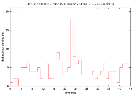
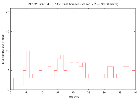
Figure 18: Two of the clusters found on January 2, 1999: a single cluster selected for $T=40$ sec (left) and the first of the clusters selected for $T=45$, 50 sec (right), see Tables 2c, 3 and the text. Notice that both clusters begin simultaneously.

• 02.01.99: Similar to the above event, the shortest cluster in this event is a single one. This cluster is shown in Fig. 18. As $T$ grows, the number of clusters increases. As one can see from Table 3, for $T=45$ and 50 sec we have found groups that contain two and three consecutive clusters respectively. It is remarkable that for each of these two groups, the first cluster appears simultaneously with the shortest one, while the right boundary of each sequence slightly moves. For both groups, the first cluster covers the range of EAS No. 4231–4250 thus containing 20 showers arriving in 48.72 sec, see Fig. 18. For this cluster, $T_{\mathrm{adj}}=44.98$ sec, $\mathcal{P}_{\mathrm{adj}}=2.8\times 10^{-8}$.

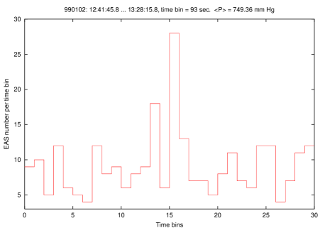
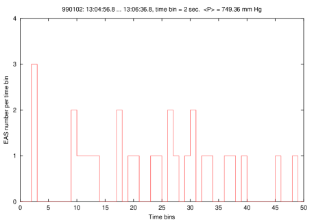
Figure 19: A single cluster found on January 2, 1999 for $T=90$ sec (left) and its “interior structure” (right), see Tables 2b and 3. Notice that the cluster selected for $T=40$ sec occupies bins No. 9–31.

  Next, for $T=55\dots 90$ sec all events begin at shower No. 4228 thus appearing nearly 14 sec earlier than the shortest cluster. It is interesting that for $T=80$ and 85 sec the first cluster begins at EAS No. 4228, while the second one is “shifted” to the EAS No. 4231, which is the first shower for the shortest cluster in this event. For $T=80$ sec, the first cluster consists of 26 EAS arriving in 75.85 sec with $T_{\mathrm{adj}}=70.03$ sec and $\mathcal{P}_{\mathrm{adj}}=1.0\times 10^{-8}$. The second cluster is a bit less intensive: it also consists of 26 EAS, but they occupy 85.96 sec with $T_{\mathrm{adj}}=79.37$ sec and $\mathcal{P}_{\mathrm{adj}}=1.1\times 10^{-7}$. No other clusters are identified between them. Finally, for $T=90$ sec a single cluster is found, see Table 2c and Fig. 19. Notice that it consists of exactly the same EAS that are covered by three clusters selected for $T=75$ sec. Notice also that the right boundary of this cluster has moved by 35.92 sec in comparison with the shortest cluster, while the left boundary has shifted by 13.95 sec only. Thus the peak count rate is closer to the beginning of the event. This is clearly seen in the figure.

  For $T=2$ and 3 min, besides other clusters, there are clusters that begin at EAS No. 4228 and 4231. For $T=2$ min, they cover the range of EAS No. 4228–4260 and 4231–4261 and contain 33 and 31 showers with $\mathcal{P}_{\mathrm{adj}}=1.0\times 10^{-7}$ and $\mathcal{P}_{\mathrm{adj}}=2.9\times 10^{-7}$ respectively. For $T=3$ min, they cover the range of EAS No. 4228–4269 and 4231–4270 and contain 42 and 40 showers with $\mathcal{P}_{\mathrm{adj}}=1.0\times 10^{-7}$ and $\mathcal{P}_{\mathrm{adj}}=7.3\times 10^{-7}$ respectively.

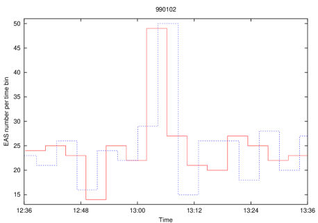
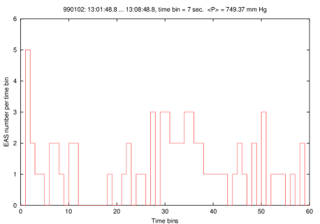
Figure 20: Left plot: two “shifted” clusters selected for $T=4$ min on January 2, 1999, see Tables 2c, 3, and the text. Time bins are equal to 257 sec. Right plot: the “interior structure” of these clusters. The first cluster occupies bins No. 2–38, the second cluster occupies bins No. 22–59. Notice that the clusters shown in Fig. 18 occupy bins No. 30–36 and 30–37 respectively.

  An interesting situation takes place for $T=4$ min. There are only three clusters in the group, and the first one covers the range of EAS No. 4204–4252. It consists of 49 showers arrived in 256.28 sec. The other two clusters cover the range of EAS No. 4223, 4224–4272 thus containing 50 and 49 showers respectively. The second cluster begins 144.95 sec later than the first one and ends 145.66 sec later (so that their durations are nearly equal), see Fig. 20. This allows us to assume that these two clusters are found not because of the search method, but may represent an astrophysical process that consists of two consecutive bursts.

  For $T=5$ min, the beginning of the group of clusters moves more to the left, so that four clusters in this group cover the range of EAS No. 4196–4253, 4197–4254, and 4203–4260, 4204–4261 respectively, thus splitting into two subgroups. Notice that the last cluster begins simultaneously with the first 4-minute cluster.

  For $T=6$ min, the group again splits into two subgroups of consecutive clusters. The first one begins at EAS No. 4195 (at 13:00:44.42) and consists of four clusters, the last of them ending at EAS No. 4263 (at 13:07:28.11). The second subgroup consists of five clusters, the first of them beginning at EAS No. 4210 (at 13:01:20.17) and the last one ending at EAS No. 4270 (at 13:08:25.23).

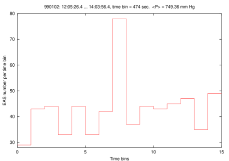
Figure 21: The widest group of clusters selected for the event registered on January 2, 1999 (left) and its “interior structure” (right). Notice that the first of the clusters selected for $T=4$ min (see Fig. 20) begins at the 6th bin of the right plot, while the second one begins at the 13th bin. Bins No. 18–20 represent the first of the clusters selected for $T=45$, 50 sec (see the right plot in Fig. 18).

  Finally, for $T=7$ min there are only five consecutive clusters. They cover the widest range of EAS arrival times that occupies nearly eight minutes, see Tables 2c, 3, and the left plot in Fig. 21. An analysis of the “interior structure” of this group of clusters clearly demonstrates how two subgroups of clusters appear in this event, see the right plot in Fig. 21.

Table 2c: Events that have a complicated structure of embedded clusters. See notation in Tables 1 and 2a.

Date	$P$,	$T$,	Beginning	End	$T_{\mathrm{real}}$,	$N_{\mathrm{EAS}}$	$N_{\mathrm{cl}}$	$T_{\mathrm{adj}}$,	$\mathcal{P}_{\mathrm{adj}}$
dd.mm.yy	mm Hg	sec	hh:mm:ss	hh:mm:ss	sec			sec
02.11.98	738.6	40	09:54:56.30	09:55:34.04	37.74	18	1	39.15	$8.3\times 10^{-8}$
		$\cdots$
		60	09:54:29.89	09:55:42.88		28	2
		$\cdots$
		90	09:54:19.67	09:55:56.61		31	4
		120	09:53:39.25	09:56:19.79		39	9
		$\cdots$
		240	09:52:22.18	09:56:19.79		50	2
02.01.99	749.4	40	13:05:14.81	13:05:57.82	43.01	18	1	39.71	$1.0\times 10^{-7}$
		$\cdots$
		65	13:05:00.86	13:06:16.71		26	4
		$\cdots$
		90	13:05:00.86	13:06:33.74	92.88	28	1	85.75	$3.9\times 10^{-8}$
		120	13:04:20.77	13:07:28.11		41	10
		$\cdots$
		240	13:01:55.82	13:08:37.76		69	3
		$\cdots$
		420	13:00:44.42	13:08:37.76		78	5
08.01.99(b)	726.7	55	00:20:50.36	00:21:36.94	46.58	21	1	54.95	$1.5\times 10^{-7}$
		60	00:20:50.36	00:21:40.29	49.93	22	1	58.90	$1.1\times 10^{-7}$
		65	00:20:22.51	00:21:33.15		30	5
		$\cdots$
		90	00:20:11.97	00:21:40.29		34	7
		120	00:19:32.48	00:21:40.29		43	13
		180	00:18:59.36	00:23:08.77		58	13
		$\cdots$
		420	00:19:32.48	00:25:49.64		79	5
		$\cdots$
		660	00:19:32.48	00:28:39.25	546.77	105	1	645.07	$1.8\times 10^{-7}$
		$\cdots$
		900	00:19:47.03	00:32:26.31	759.28	134	1	895.75	$4.0\times 10^{-7}$

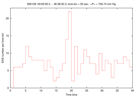
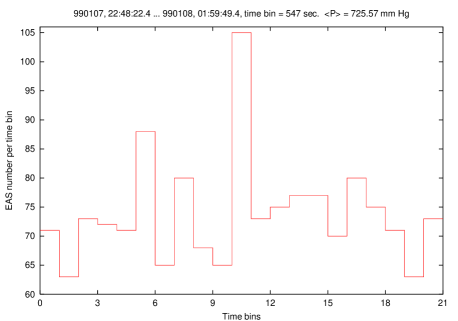
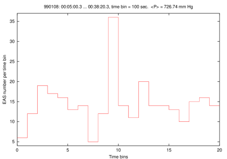
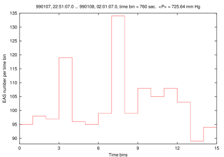
Figure 22: Some of the clusters that constitute an event registered on January 8, 1999(b), see Tables 2c and 3. Top row: single clusters found for $T=60$ sec and $T=11$ min. Bottom row: the eighth of the clusters selected for $T=2$ min and a single cluster found for $T=15$ min. Notice that clusters in the left column end simultaneously.

• 08.01.99(b): This is an event with the biggest number of clusters. As one can see from Table 3, separate clusters are found for $T=55$ and 60 sec and for $T=11$ and 15 min. The last three clusters are shown in Fig. 22. Surprisingly enough, but no clusters were found for $T=6$ and 13 min.

  If we compare the clusters selected for $T=55$ and 60 sec with longer ones then we find that for $T=65\dots 90$ sec, the left boundary of the sequences of clusters is shifted from EAS No. 164 to EAS No. 152–154, while the right boundary remains practically unchanged, see Tables 2c and 3. Beginning with $T=2$ min, the left boundary of the selected groups jumps further to EAS No. 141–145. Then at $T=3$ min, the right boundary begins to move considerably to the right. It is interesting to notice that while the right boundary moves monotonically as $T$ grows, the left boundary fluctuates around EAS No. 143, so that the longest group ($T=15$ min) appears later than the majority of the groups selected for $T=2\dots 14$ min.

Table 3: Three events with a complicated structure of embedded clusters. For each event, the first number gives the number of clusters for a given $T$; letter “c” means that the corresponding clusters begin at consecutive arrival times. Then the range of EAS numbers for each event follows.

$T$		02.11.98		02.01.99		08.01.99(b)
40	sec	1 :	3723–3740	1 :	4231–4248
45		4c:	3723–3744	2c:	4231–4250
50		3c:	3723–3744	3c:	4231–4252
55		2c:	3723–3744	4 :	4228–4253	1 :	164–184
60		2 :	3717–3744	4 :	4228–4253	1 :	164–185
65		4 :	3717–3745	4c:	4228–4253	5 :	154–183
70		5 :	3715–3744	4c:	4228–4254	6 :	153–184
75		5c:	3716–3744	3 :	4228–4255	8 :	153–185
80		5c:	3715–3744	2 :	4228–4256	9c:	152–185
85		4c:	3715–3744	2 :	4228–4257	7c:	153–185
90		4c:	3715–3745	1 :	4228–4255	7c:	152–185
2	min	9c:	3710–3748	10c:	4223–4263	13c:	143–185
3		7 :	3701–3748	8 :	4223–4270	13 :	141–198
4		2c:	3699–3748	3 :	4204–4272	10c:	143–200
5				4 :	4196–4261	5 :	141–203
6				9 :	4195–4270
7				5c:	4195–4272	5 :	143–221
8						7c:	143–230
9						5 :	143–237
10						7c:	143–245
11						1 :	143–247
12						3c:	145–258
13
14						3c:	143–271
15						1 :	145–278

• Some of the clusters that form the groups found for $T=2$ and 3 min are really remarkable. In particular, the fourth of the clusters selected for $T=2$ min begins at EAS No. 146 (at 00:19:52.63) and consists of 38 showers arriving in 100.51 sec with $T_{\mathrm{adj}}=118.58$ sec and $\mathcal{P}_{\mathrm{adj}}=3.1\times 10^{-10}$; the cluster ends simultaneously with a group found for $T=65$ sec and contains it inside itself. There is another cluster inside this one: it begins at EAS No. 147 and ends simultaneously with the outer cluster. For this cluster, $T_{\mathrm{adj}}=116.19$ sec, $\mathcal{P}_{\mathrm{adj}}=6.1\times 10^{-10}$. The eighth cluster is also worth mentioning: it begins at EAS No. 150 and consists of 36 showers arriving in 99.19 sec with $T_{\mathrm{adj}}=117.03$ sec and $\mathcal{P}_{\mathrm{adj}}=2.4\times 10^{-9}$. This cluster ends simultaneously with the single cluster selected for $T=60$ sec, see the left bottom plot in Fig. 22.

  For $T=3$ min, there is a cluster with an extremely small $\mathcal{P}_{\mathrm{adj}}=2.3\times 10^{-10}$. It covers the range of EAS No. 145–185 and consists of 41 showers arriving in 113.25 sec with $T_{\mathrm{adj}}=133.62$ sec. It is remarkable that this cluster begins simultaneously with the cluster selected for $T=15$ min and ends simultaneously with the one found for $T=60$ sec.

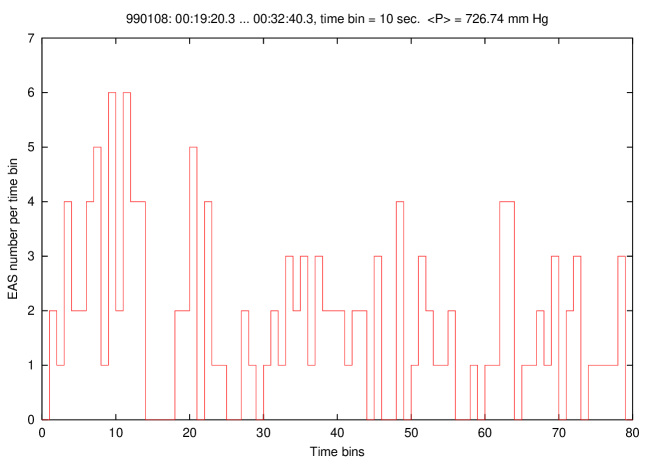
Figure 23: The “interior structure” of the outer cluster found for the event registered on January 8, 1999(b). Bins No. 10–14 represent the single cluster selected for $T=60$ sec, see Table 2c and Fig. 22. Bins No. 5–14 represent the eighth of the clusters selected for $T=2$ min; the whole group occupies bins No. 2–14. Bins No. 39 and 56 are the last bins for the clusters found for $T=7$ and 11 min respectively.

  The groups selected for $T>3$ min do not contain any outstanding clusters. Thus we assume that this event is presented by the cluster selected for $T=15$ min with the peak count rate located at the most intensive interior clusters, see Fig. 23 for the “substructure” of this cluster.

Now we see that though the presented clusters have been selected by the same formal procedure, they are not identical but differ in a considerable number of properties such that the duration, the interior structure, the location of the peak count rate, etc. It seems to be a great challenge to try to figure out which astrophysical events are responsible for the observed EAS clusters and the variety of their properties.

3 Arrival Directions of EAS in Clusters

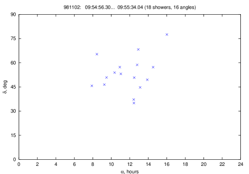
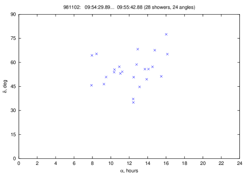
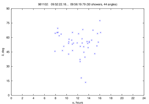
Figure 24: Arrival directions of EAS in the cluster event registered on November 2,1998. One can see how showers with close arrival directions appear if an interior cluster is compared with an outer one, see Tables 2b and 2c. The titles of the plots contain the total number of showers in a cluster and the number of arrival directions (“angles”) determined.

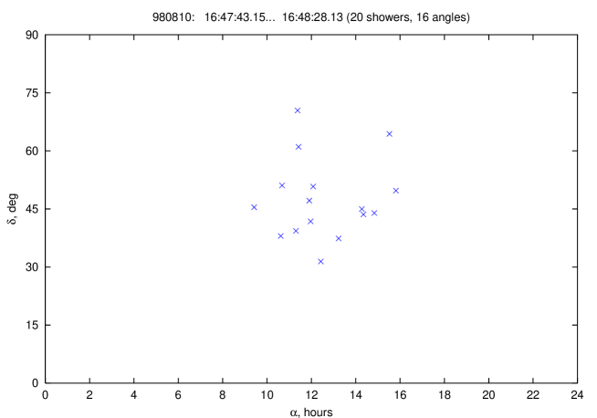
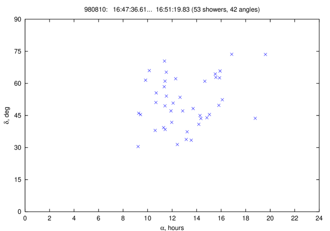
Figure 25: Arrival directions of EAS in the cluster event registered on August 10, 1998.

As soon as one finds an EAS cluster, a natural question arises: Do any of the showers that form a cluster have the same astrophysical source, i.e., do they have the same arrival direction? As one can see from Figs. 24, 25, and 26, the majority of showers in a cluster do not have a joint source. (We recall that Japanese researchers have come to a similar conclusion [1, 2, 3].) On the other hand, one can often find pairs and sometimes even triplets of showers that have very close or coincident arrival directions. The number of such groups grows for clusters that consist of a sufficiently large number of showers. Figs. 24 and 25 show how the number of EAS with close arrival directions grows if an interior cluster is compared with an exterior one. This leads us to the conjecture that a part of showers in a cluster may have common sources. Nevertheless, we must remark that a similar situation sometimes takes place for samples that do not form a cluster. Thus this is an open question to be clarified in a future investigation: Do pairs and triplets of showers with close arrival directions found in some clusters have purely statistical origin or not?

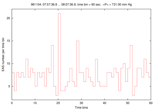
Figure 27: An event registered on November 4, 1998, cf. Fig. 12. The top plot: the count rate during an hour time interval. The bottom plot: arrival directions of EAS that constitute the cluster ($\vartriangle$) and three peaks located at 29th, 37th, and 52th bins ($\times$, $+$, and $\circ$ respectively).

It should be marked that as a rule the clusters represent single “bursts” of the count rate in a sense that there are no other bursts around. In view of this fact, an event with some kind of an “afterglow” seems to be especially interesting. It has been registered on November 4, 1998 (one of the events with a “simple embedding,” see above). As it is clearly seen from Fig. 27, this cluster is accompanied by a sequence of less intensive “bursts.” This figure also shows arrival directions of EAS that form the cluster and three following peaks (located at 29th, 37th, and 52th bins). One can see that the cluster has showers that are close to the showers in the first and the third peaks; these peaks also have EAS with close arrival directions. It is also interesting that time intervals between the peak that contains the cluster and three highest peaks that follow it are equal to 7, 7, and 14 minutes.

One can also see a “burst” that precedes the cluster. It also contains showers that have arrival directions close to some of the EAS in the following peaks. In our opinion, this may be a manifestation of some astrophysical event.

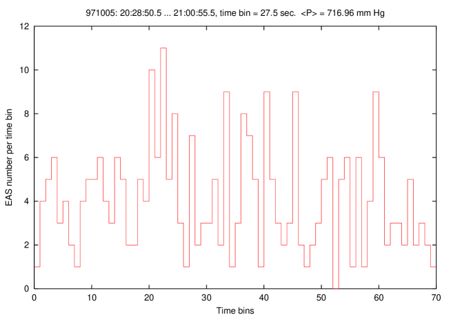
Figure 28: An event registered on October 5, 1997, cf. Fig. 5. The top plot: the count rate during a 32-minute time interval; the cluster occupies bins No. 20–25. The bottom plot: arrival directions of EAS that constitute the cluster ($\bullet$) and those that belong to bins No. 28 ($\times$), 34 ($+$), 41 and 42 ($\circ$), 46 ($\Box$), 60 and 61 ($\vartriangle$).

A similar phenomenon can be observed for the event registered on October 5, 1997, see Table 2a and Fig. 5. This time, the “afterglow” is observed if one studies the “interior structure” of the cluster, see Fig. 28. Namely, if we consider the count rate at a time interval that contains the cluster using comparatively small time bins (approximately in the range 25–55 sec) then we observe a sequence of peaks that follow the cluster. It is remarkable that some of EAS that form these peaks have arrival directions close to those of the EAS that form the cluster (arrival directions were determined for 32 of 40 showers in the cluster). Namely, as one can see from Fig. 28, at least ten of the EAS in the cluster have close counterparts from the following peaks: there are six pairs, three triplets, and a quadruplet. It is interesting that if we add arrival directions of EAS that form peaks at bins No. 37–39 then we find only one more pair. It is also important that if we compare arrival directions of EAS that form the cluster with arrival directions of the following 150 EAS (thus covering all 9-shower peaks shown in Fig. 28) then we find that almost all showers with arrival directions close to that of the cluster belong to the selected peaks. In our opinion, the observed sequence of short “bursts” can be caused by a common astrophysical process.

Another interesting phenomenon revealed by our analysis is the fact that showers that form different clusters can also have close arrival directions. For instance, we have found numerous showers with nearly coincident arrival directions in the cluster events registered on 01.05.98, 10.08.98, 02.11.98, 04.11.98, 08.01.99(a) and 09.04.98, 16.08.98, 08.11.98, 28.12.98, 03.01.99, see Fig. 29. Notice in particular that there are five showers with very close arrival directions in the upper plot (around $\alpha=9.43$ hour, $\delta=46^{\circ}$). In our opinion, this finding can give a clue to the search of point sources of cosmic rays with the energy $\sim 10^{15}$ eV.

Finally, a few remarks concerning the electron number $N_{e}$ in EAS that form clusters are in order. As we have already mentioned above, the mean value $\bar{N}_{e}$ for the whole data set under consideration approximately equals $1.2\times 10^{5}$. For the clusters presented in Tables 2a–c, $\bar{N}_{e}$ has the same order of magnitude. The most energetic showers were found within clusters registered on November 11, 1998 and January 6, 1999(b) with $N_{e}\approx 10^{6}$ particles. Slightly less powerful showers with $N_{e}\approx 5\div 7\times 10^{5}$ were detected within clusters registered on December 24 and 28, 1998, November 8, 1998, and January 3, 1999.

4 Discussion

It is interesting to compare the results of our investigation with results obtained at other experimental EAS arrays. Unfortunately, we have found very few results of similar investigations undertaken during the same period of data collection. The authors of [19] studied sequences of EAS arrival times that demonstrated chaotic behavior. Among the data they present, we find two events that were registered during the days which are also present in our data set (namely, those registered on 15.05.98 and 01.08.98). A similar investigation presented in [20] also contains an event observed on a day present in our data (11.04.98). A comparison did not reveal any correlation between these events and our results of clusters search. This seems to be quite natural since the energy of the events under consideration is comparatively low. Finally, the results presented by the LAAS group [21] contain seven successive air shower (SAS) events observed during the period covered by our data set. SAS events are defined as sequences of EAS detected within a short time interval and thus may be called clusters in our terminology. It is interesting that two of the SAS events have arrival time comparatively close to that of the clusters we have found on August 16, 1998 and January 8, 1999. A question whether there may be some correlation between these events needs to be studied in details.

Besides this, we have studied ultrahigh energy events ($>4\times 10^{19}$ eV) registered with the AGASA array either [18]. Again, two of the AGASA events were registered during the days that belong to our data set (04.04.98 and 27.10.98). For these days, our data contain a number of EAS with arrival directions close to the arrival directions of the corresponding AGASA event, but there are no coincidences between these events and EAS clusters we selected, since these days do not contain EAS clusters. Still, we have found that there is some interesting correlation between arrival direction of the C2 triplet of the AGASA events and arrival directions of showers in several EAS clusters, see Fig. 30. It is worth recalling that this AGASA triplet is located near the supergalactic plane in the direction of the Ursa-Major II cluster of galaxies and near such astrophysical objects as NGC 3642, Mrk 40, and Mrk 171 [18].

Finally, we have compared our EAS clusters with the gamma-ray bursts (GRBs) registered by BATSE [22]. In total, we have found 78 GRBs in the BATSE Catalog that have a positive value of declination $\delta$ and which were registered during the days present in our data set. (One of them has also been analyzed within Project GRAND [23], namely the one registered on April 20, 1998.) Nine of these GRBs were observed during the days when EAS clusters were registered, though four of them have arrived before the corresponding cluster.

To obtain a more detailed understanding of possible correlation between GRBs and EAS, we have analyzed our data looking for EAS that have arrival times close to the corresponding GRB and arrival directions that deviate from the GRB coordinates at most by $6^{\circ}$ in declination $\delta$ and by $6/\cos(\delta)$ in right ascension $\alpha$ (the division by the cosine was used to have an equivalent area of the window for all $\delta$). We have found that for 62 GRBs there is at least one EAS with a close arrival direction and registered during the same day. (It is necessary to mention that though the arrival direction is usually determined for the majority of registered EAS, there are always a number of showers with an unknown arrival direction. Thus the number of EAS with arrival directions close to the corresponding GRB may be bigger.) For 31 GRBs there are more than 60 EAS with close arrival directions, and 16 GRBs have more than 100 close EAS (up to 137). Among them, there are 11 GRBs that have one or more EAS counterparts within a 200-second interval. For six of these events, the deviation in coordinates does not exceed 2–3^∘. Recall that the geometry of the EAS-1000 prototype array allows one to determine arrival directions of EAS with an error of the order of $5^{\circ}$. Hence the difference in arrival directions of these GRBs and the corresponding EAS is really small.

It is interesting to note that for the above mentioned 62 GRBs the corresponding sequences of showers often contain a number of doublets and even triplets of EAS registered within a short period of time. This finding gives rise to another problem to be studied, namely to analyze the distribution of arrival times of these EAS. This may give useful information for the search of point sources of both EAS and GRBs.

Concerning the EAS clusters discussed above, we have found that the cluster registered on January 2, 1999 contains a shower with the arrival direction close to that one of the GRB No. 7293: the GRB has $\alpha=277^{\circ}$, $\delta=39^{\circ}$, while the corresponding EAS has $\alpha=271^{\circ}$, $\delta=45^{\circ}$. On the other hand, there are no EAS that have arrival directions close to that of the GRB and registered at the time of the GRB observation.

The most interesting GRB/EAS-cluster pair is the one registered on December 28, 1998. The first shower in the EAS cluster has arrived approximately one minute before the trigger time of the GRB No. 7285. In this connection, recall that the BATSE Catalog, besides other information, provides ST90 (start time for the T90 interval relative to the trigger time) and T90 (the duration of time after ST90 which includes 90% of the total observed counts in the GRB). For the GRB No. 7285, ST$90=-77.824$ sec and T$90=156.096$ sec with the uncertainty equal to $1.590$ sec. Thus this GRB begins by 14.6 sec earlier than the EAS cluster, and the time interval of the GRB observation contains the time interval of the EAS cluster registration.

In connection with this pair, let us also mention that the GRB No. 7285 has the equatorial coordinates $\alpha=286^{\circ}$ and $\delta=31^{\circ}$. In its turn, the EAS cluster contains a shower with $\alpha=279^{\circ}$ and $\delta=29^{\circ}$. Taking into account the precision of the EAS–1000 prototype array, we assume that these arrival directions are close.

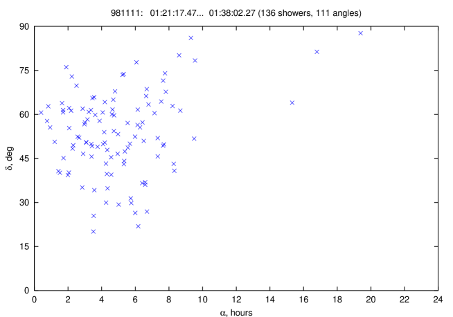
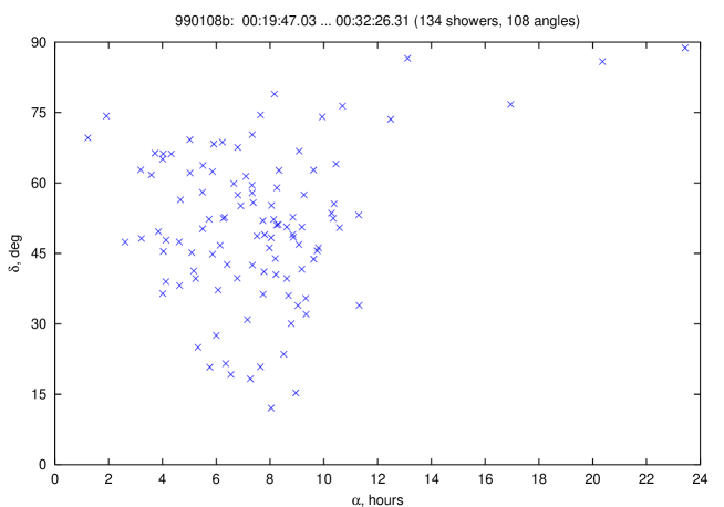
Figure 26: Arrival directions of EAS in two longest events (11.11.98 and 08.01.99(b), see Tables 2b and 2c). One can see pairs and triplets of showers with almost coincident arrival directions.

We would also like to mention a situation that takes place with the EAS cluster registered on 11.11.98 (see Table 2b and the discussion above) and the GRB No. 7207. This GRB was registered more than eight hours later than the EAS cluster (the trigger time equals 09:43:40.90). The EAS data set does not contain any shower with an arrival direction close to this GRB within an hour time interval. As for the cluster, it consists of 136 EAS, and the arrival directions are known for 111 of them (see Fig. 26). To compare, 353 EAS were registered within the hour 01:00…02:00 (Moscow local time), the arrival directions were determined for 299 of them, 13 of them are close to that of the GRB, and 8 belong to the cluster. Thus we see some excess of EAS with arrival directions close to the GRB within a cluster. It is interesting, whether this can be a manifestation of an astrophysical process.

Thus we think that there may be certain correlation between GRBs and EAS clusters and even single EAS generated by cosmic rays with the energy $\sim 10^{15}$ eV. A more detailed analysis of the arrival directions and moments of registration of EAS and the corresponding GRBs is planned to be carried out to verify this hypothesis.

5 Conclusion

The analysis of arrival times of extensive air showers registered with the EAS–1000 prototype array has revealed a number of events that may be identified as clusters. The discovery of these events gives rise to numerous questions in both statistics and phenomenology. First of all, it is a question about possible sources and physical reasons of cluster appearance, and their connection with other astrophysical phenomena. The presented results demonstrate that there may be a correlation between some GRBs, ultrahigh energy events, and clusters of EAS with mean electron number of the order of $10^{5}$ particles.

One of the most promising approaches in future study of EAS arrival times and in particular the clusters we have already found is an application of methods of the nonlinear time series analysis (see, e.g., [24, 25, 26, 27, 28]). A preliminary investigation based on fractal analysis approach has revealed that some of EAS clusters demonstrate signs of chaotic dynamics. These results will be presented elsewhere [29].

A separate problem is connected with the distribution of arrival times of showers that form a cluster. As it was shown above, the position of the highest count rate may vary in different clusters. By the moment, we did not find a statistical distribution that is valid for all clusters. A study of this question is in the plan of our future research, especially in connection with the clusters that contain a sufficiently big number of EAS.

Finally, our investigation has also revealed a number of superclusters—EAS clusters that have duration more than 30 min. As a rule, they do not contain short embedded clusters. But two of the clusters given in Tables 2b and 2c belong to the corresponding superclusters. A detailed analysis of superclusters may be the subject of a separate investigation.

Figures

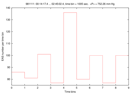
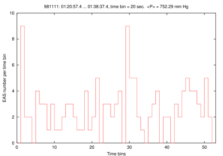
Figure 15: An event registered on November 11, 1998, see Table 2b, and its “substructure.”

Figure 29: Close arrival directions of EAS in different clusters.

Figure 30: Arrival directions of EAS in four clusters and the C2 cluster of AGASA events ($\bullet$) [18].

References

- [1] M. Chikawa, T. Kitamura, T. Konishi, K. Tsuji, “An analysis of candidates of non-random component in extensive air showers above 0.1 PeV at sea level,” Proc. 22nd ICRC, Dublin, 4, 287–290, 1991.
- [2] K. Tsuji, T. Konishi, T. Kitamura, M. Chikawa, “Search for bursts of extensive air showers by adaptive cluster analysis,” Proc. 23rd ICRC, Calgary, 4, 223–226, 1993.
- [3] Y. Katayose, Y. Inoue, Y. Kawasaki et al., “Search for bursts of extensive air showers,” Proc. 24th ICRC, Rome, 1, 305–308, 1995.
- [4] N. Ochi, A. Iyono, T. Nakatsuka et al., “Study of the arrival time structure of serial air showers,” Proc. 27th ICRC, Hamburg, 2001, 1, 193–194.
- [5] N. Ochi, T. Wada, Y. Yamashita et al., “Search for non-random features in arrival times of air showers,” Nuovo Cim. 24C (2001) 719–723.
- [6] O. V. Vedeneev, N. N. Kalmykov, G. V. Kulikov et al., “Arrival time distribution of extensive air showers,” Izv. Ros. Akad. Nauk, Ser. Fiz. 65 (2001) 1224–1225 [Bull. Rus. Acad. Sci., Ser. Phys.].
- [7] Yu. A. Fomin, N. N. Kalmykov, G. V. Kulikov et al., “Distribution of EAS arrival times according to data of the EAS-1000 Prototype array,” Proc. 27th ICRC, Hamburg, 2001, 1, 195–196; astro-ph/0201343.
- [8] T. Maeda, H. Kuramochi, S. Ono et al., “The arrival time distribution of EAS at Taro,” Proc. 27th ICRC, Hamburg, 2001, 1, 189–192.
- [9] S. S. Ameev, I. Ya. Chasnikov, Yu. A. Fomin et al., “EAS–1000. Status 1997,” Proc. 25th ICRC, Durban, 1997, 7, 257–260.
- [10] Yu. A. Fomin, A. V. Igoshin, N. N. Kalmykov et al., “New results of the EAS-1000 Prototype operation,” Proc. 26th ICRC, Salt Lake City, 1999, 1, 286–289.
- [11] V. B. Atrashkevich, O. V. Vedeneev, A. V. Igoshin et al., “Prototype of the EAS-1000 array. The first results,” Preprint 98-53/554, Skobeltsyn Institute of Nuclear Physics at Moscow State University, Moscow, 1998, 50 pp. (in Russian).
- [12] O. V. Vedeneev, Yu. A. Fomin, G. V. Kulikov, M. Yu. Zotov, “EAS clusters with ,” Izv. Ros. Akad. Nauk, Ser. Fiz. 65 (2001) 1653–1656 [Bull. Rus. Acad. Sci., Phys. Ser.].
- [13] T. Anderson, The Statistical Analysis of Time Series, New York, Wiley, 1971.
- [14] J. S. Bendat, A. G. Piersol, Random Data: Analysis and Measurement Procedure, New York, Wiley, 1986.
- [15] Yu. N. Tyurin, A. A. Makarov, Computer-based Statistical Analysis of Data, Moscow, Infra-M, 1998 (in Russian).
- [16] L. N. Bol’shev, N. V. Smirnov, Tables of Mathematical Statistics, Moscow, Nauka, 1983.
- [17] J. W. Eaton, “GNU Octave: A high-level interactive language for numerical computations,” Edition 3 for version 2.0.13, 1997; http://www.che.wisc.edu/octave/
- [18] M. Takeda, N. Hayashida, K. Honda et al., “Small-scale anisotropy of cosmic rays above eV observed with the Akeno Giant Air Shower Array,” Astrophys. J. 522 (1999) 225–237. Y. Uchihori, M. Nagano, M. Takeda et al., “Cluster analysis of extremely high energy cosmic rays in the northern sky,” Astropart. Phys. 13 (2000) 151–160. N. Hayashida, K. Honda, N. Inoue et al., “Updated AGASA event list above eV,” astro-ph/0008102. M. Takeda, M. Chikawa, M. Fukushima et al., “Clusters of cosmic rays above eV observed with AGASA,” Proc. 27th ICRC, Hamburg, 2001, 1, 341–344.
- [19] T. Harada, S. Chinomi, K. Hisayasu et al., “Fractal study of extensive air showers time series,” Proc. 26th ICRC, Salt Lake City, 1999, 1, 309–312. S. Saito, S. Chinomi, T. Harada et al., “Fractal study of extensive air showers time series,” Proc. 27th ICRC, Hamburg, 2001, 1, 212–215.
- [20] S. Ohara, T. Konishi, K. Tsuji et al., “The periodicity of the cosmic ray chaos,” Proc. 26th ICRC, Salt Lake City, 1999, 3, 244–247.
- [21] N. Ochi, T. Wada, Y. Yamashita et al., “Anisotropy of successive air showers,” Nucl. Phys. B (Proc. Suppl.) 97 (2001) 173–176.
- [22] The BATSE Gamma Ray Bursts Catalogs, http://www.batse.msfc.nasa.gov/batse/
- [23] T. F. Lin, J. Carpenter, S. Desch et al., “Possible detection of gamma ray air showers in coincidence with BATSE gamma ray bursts,” Proc. 26th ICRC, Salt Lake City, 1999, 4, 24–27; astro-ph/005180. J. Poirier, T. F. Lin, J. Gress et al., “Sub-TeV gammas in coincidence with BATSE gamma ray bursts,” astro-ph/0004379.
- [24] J.-P. Eckmann, D. Ruelle, “Ergodic theory of chaos and strange attractors,” Rev. Mod. Phys. 57 (1985) 617–656.
- [25] J. Theiler, “Estimating fractal dimension,” J. Opt. Soc. Am. A7 (1990) 1055–1073.
- [26] H. Kantz, T. Schreiber, Nonlinear Time Series Analysis, Cambridge Univ. Press, Cambridge, 1997.
- [27] T. Schreiber, “Interdisciplinary application of nonlinear time series methods,” Phys. Reports 308 (1999) 1–64; chao-dyn/9807001.
- [28] G. G. Malinetskii, A. B. Potapov, Modern Problems of Nonlinear Dynamics, Moscow, URSS, 2000 (in Russian).
- [29] Yu. A. Fomin, G. V. Kulikov, M. Yu. Zotov, “Nonlinear analysis of EAS clusters,” to appear, see the astro-ph archive.