The luminosity functions and stellar masses of galactic disks and spheroids

Abstract

We present a method to obtain quantitative measures of galaxy morphology and apply it to a spectroscopic sample of field galaxies in order to determine the luminosity and stellar mass functions of galactic disks and spheroids. For our sample of approximately 600 galaxies we estimate, for each galaxy, the bulge-to-disk luminosity ratio in the I-band using a two-dimensional image fitting procedure. Monte Carlo simulations indicate that reliable determinations are only possible for galaxies approximately two magnitudes brighter than the photometric completeness limit, leaving a sample of 90 galaxies with well determined bulge-to-total light ratios. Using our measurements of individual disk and bulge luminosities for these 90 galaxies, we construct the luminosity functions of disks and spheroids and, using a stellar population synthesis model, we estimate the stellar mass functions of each of these components. The disk and spheroid luminosity functions are remarkably similar, although our rather small sample size precludes a detailed analysis. We do, however, find evidence in the bi-variate luminosity function that spheroid-dominated galaxies occur only among the brightest spheroids, while disk-dominated galaxies span a much wider range of disk luminosities. Remarkably, the total stellar mass residing in disks and spheroids is approximately the same. For our sample (which includes galaxies brighter than $M_{*}+2$, where $M_{*}$ is the magnitude corresponding to the characteristic luminosity), we find the ratio of stellar masses in disks and spheroids to be $1.3\pm 0.2$. This agrees with the earlier estimates of Schechter & Dressler, but differs significantly from that of Fukugita, Hogan & Peebles. Ongoing large photometric and redshift surveys will lead to a large increase in the number of galaxies to which our techniques can be applied and thus to an improvement in the current estimates.

1 Introduction

It has long been known that galaxies in the nearby Universe display a range of morphological characteristics that distinguish between disk-dominated (e.g. spiral) and spheroid-dominated (e.g. elliptical) galaxies, with many fine subdivisions within each class (e.g. Hubble 1926; de Vaucouleurs 1959). The origins of these different types of galaxy and the evolutionary connections, if any, between them are still unclear, although there is a wealth of observational data and several proposed theories.

Traditionally, morphology has been assigned by human classifiers directly from galaxy images, a process that is accurate only to within about two T-types (Naim et al., 1995). More recently, computer-based algorithms have been developed which show a reasonable correlation with “eyeball” estimates, at least for bright galaxies (e.g. Abraham et al. 1996). Unfortunately, all these classifications tend to give considerable weight to detailed morphological features, such as spiral arms or asymmetries in the image, and are difficult to compare with current theoretical predictions which focus on simpler quantities such as the total stellar mass or luminosity in the disk and spheroidal components. Here, we consider a morphological quantifier that is more easily related to theoretical models.

It is widely believed that disks form by slow accretion of gas which acquired angular momentum through tidal torques (Hoyle, 1949; Peebles, 1969), although whether this picture works in detail remains an open question (Navarro, Frenk & White, 1995; Navarro & Steinmetz, 1997, 2000; van den Bosch, Burkert & Swaters, 2001). Spheroids, on the other hand, are thought to form either by a “monolithic collapse” (Eggen, Lyden-Bell & Sandage, 1962; Jimenez et al., 1999), or as a result of mergers of pre-existing galaxies (Toomre 1977; Barnes & Hernquist 1992 and references therein). Detailed theoretical predictions for the statistical morphological properties of galaxies and their evolution have been calculated for the hierarchical merging formation mechanism appropriate to cold dark matter cosmologies (Kauffmann, White & Guiderdoni, 1993; Kauffmann, 1995, 1996; Baugh, Cole & Frenk, 1996a,b; Somerville, Primack & Faber, 2001). Among other things, these models give the relative luminosities and stellar masses of the spheroids and disks of galaxies.

In this work, we measure the I-band bulge-to-total light ratio, B/T, for a large sample of galaxies with spectroscopic redshifts by fitting two-dimensional models to the observed galaxy images. We use this information to estimate the spheroid and disk luminosity functions, as well as the total stellar mass that resides in disks and spheroids. An earlier attempt to estimate the relative contributions to the luminosity from spheroids and disks was carried out by Schechter & Dressler (1987), based on “eyeball” estimates of the bulge-to-total ratio.

The remainder of this paper is arranged as follows. In §2 we describe our basic dataset. In §3 we introduce the method used to fit model images to the data and thereby extract B/T (along with other interesting parameters) and describe how we estimate errors. In §4 we examine the accuracy of our technique and determine how well the B/T ratio can be measured as a function of the apparent magnitude of a galaxy. We then compute luminosity functions and total stellar masses for spheroids and disks. Finally, in §5 we present our conclusions.

2 Data

The galaxy sample used in this work is that of Gardner et al. (1997). The reader is referred to that work for a full description of the data. Here we summarize the most important features of the dataset.

Imaging of two fields of total area $10$ deg² was carried out in the B, V and I bands using the T2KA camera on the Kitt Peak National Observatory (KPNO) 0.9-m telescope, resulting in images with $0.68$-arcsec per pixel. Exposures of 300s reached $5\sigma$ detection depths of B=21.1, V=20.9 and I=19.6 in 10-arcsecond circular apertures. Imaging was also carried out in the K-band using the IRIM camera on the KPNO 1.3-m telescope resulting in 1.96-arcsecond per pixel images, and a $5\sigma$ detection depth of K=15.6 in a 10-arcsecond circular aperture. The positions of the fields were chosen randomly (the field centers are RA 14^h15^m, Dec. $+00^{\circ}$ and RA 18^h0^m, Dec. $+66^{\circ}$). The I-band images, which we will use in this work, were bias-subtracted, flattened using twilight flats and with median sky flats. Objects were identified with the sextractor program (Bertin & Arnouts 1996), using a $3\sigma$ threshold. The seeing in the optical images varied in the range $1.3<{\rm FWHM}<2.0$ arcsec. One field contained a nearby rich galaxy cluster.

Spectroscopic follow-up was obtained for a K-selected sample in sub-regions of total area $4.4$ deg², using the Autofib-2 fiber positioner and WYFFOS spectrograph on the 4.2m William Herschel Telescope on La Palma. Spectra were obtained for 567 galaxies with K$<15$, which allowed redshifts to be measured for 510 galaxies (a redshift completeness of 90%). Although the spectroscopic sample is K-selected, this does not introduce any incompleteness in the I$<16$ sample used extensively in this work (i.e. there are no galaxies with I$-$K$<1$ in the sample). We also briefly consider an I$<18$ sample, for which the spectroscopic completeness falls to around 50% because of the K-band selection (which also introduces a bias in this fainter sample against objects that are blue in I$-$K). For the I$<16$ and I$<18$ samples the median redshift is $z=0.08$ and $0.14$ respectively.

3 Method

Wadadekar, Robbason & Kembhavi (1999) have proposed a two-dimensional galaxy decomposition technique that can efficiently recover B/T ratios (and other parameters) of model galaxy images with high accuracy (see also Byun & Freeman 1995; de Jong 1996). They present a detailed study of the effects of uncertainties in the point spread function (PSF), the presence of nearby stars and the stability of the B/T estimates as a function of signal-to-noise. Our approach is similar to theirs, but we apply the technique to a large photometric sample of real galaxies. We consider the “real-world” problems of automated masking of nearby galaxies and stars and make a thorough assessment of the errors in the measured parameters. We also present, in an Appendix, estimators for the luminosity functions of disks and spheroids.

For this analysis, we have used the sample of 636 ${\rm I}<18$ galaxies of Gardner et al. (1997) imaged in B, V, I and K, as described in §3. Postage stamp images of $33\times 33$ pixels ($0.68^{{}^{\prime\prime}}$/pix) around each galaxy were extracted from the I-band data. This was the best observed band by Gardner et al. (1997) and is particularly well-suited for our purposes because it minimizes the effects of young blue stars. This image size is large enough to include the entire region of the galaxy for which reasonable signal-to-noise is achieved (and in most cases extends well beyond it.) To determine the bulge-to-total ratio, B/T, we fit the two-dimensional surface brightness profile of each galaxy using a combination of an exponential disk,

$$\Sigma_{\rm d}(\theta)=\Sigma_{\rm d,0}\exp(-\theta/\theta_{\rm d}),$$ (1)

and an $r^{1/4}$-law spheroid,

$$\Sigma_{\rm s}(\theta)=\Sigma_{\rm s,e}\exp(-7.67[(\theta/\theta_{\rm e})^{1/4}-1]),$$ (2)

where $\theta$ is the angular distance from the galaxy center. We will also consider a more general $r^{1/n}$ spheroid profile, as Wadadekar, Robbason & Kembhavi (1999) did. The disk is allowed to be inclined, and to have arbitrary position angle. The spheroid is allowed an ellipticity (defined as the ratio of semi-major to semi-minor axes) in the range 1 to 6, and can also have an arbitrary position angle. To mimic seeing, we construct mock images using these profiles which we then smooth with a Gaussian filter (integrated over each pixel to account for the variation of the PSF across the pixel),

$$p(\theta)=\exp[-(\theta/\sigma)^{2}/2]/2\pi\sigma^{2}.$$ (3)

The width of the Gaussian is treated as a free parameter, to account for variations in seeing between the images. (We will examine in §4.1 the effect of using a more realistic PSF.) The postage stamp images were centered on the galaxy of interest, but we allow the position of the image center to vary since in many cases the resulting sub-pixel variations lead to lower values of $\chi^{2}$. We also allow a small contribution from a faint, constant surface brightness background in order to take into account small inaccuracies in sky subtraction. The best fitting parameters for each galaxy were then obtained by minimizing $\chi^{2}$ using Powell’s algorithm (Brent, 1973). There are a total of 12 fit parameters (13 if we include $n$ when fitting $r^{1/n}$ spheroid profiles) summarized in Table 1. In §4.1 we will consider how accurately this procedure recovers the B/T ratio of the galaxies.

Table 1: The parameters used to construct mock galaxy images in the fitting procedure. Each parameter is described in the text.

$\Sigma_{\rm d,0}$	Disk central surface brightness
$\Sigma_{\rm s,e}$	Spheroid surface brightness at the effective radius
$\theta_{\rm d}$	Disk angular scalelength
$\theta_{\rm e}$	Spheroid effective radius
$P_{\rm d}$	Disk position angle
$P_{\rm s}$	Spheroid position angle
$i$	Disk inclination angle
$e$	Spheroid ellipticity
$(x,y)$	Center of image
$B$	Excess background surface brightness
$\sigma$	Seeing (c.f. eqn. 3)
$n$	Spheroid profile index (fixed at $n=4$ unless otherwise stated)

A significant fraction of the postage stamp images was contaminated by a secondary galaxy (and occasionally by more than one). We use a simple algorithm to identify such contaminants and mask them from the image. The aim is to remove objects which are physically distinct from the galaxy of interest without masking any pixels of the galaxy itself. We first rank the pixels in the image by surface brightness and then proceed to find groups of bright pixels. The brightest pixel is assigned to the first group. Successive pixels are assigned to a pre-existing group if they touch it (i.e. if they are adjacent either horizontally, vertically or diagonally), or else are assigned to a new group. In the case where a pixel touches more than one group, the two groups are merged. This process is continued until pixels of a fixed signal-to-noise are reached (specifically, we consider only pixels more than $3\sigma$ above the sky background). If more than one group exists at this point, the group at the center is deemed to be the galaxy of interest and the pixels of all secondary groups are marked as being contaminated and are not included in the $\chi^{2}$ sum. This simple algorithm works well in the majority of cases, but it fails in a few (28 out of 636 galaxies), either by not removing a contaminating galaxy, or by removing a significant fraction of the primary galaxy. Rather than attempting to use a more complex algorithm in these cases, we resorted to cleaning the image by hand (i.e. we view the image and manually mark the contaminated pixels).

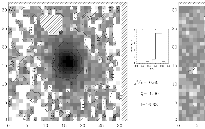
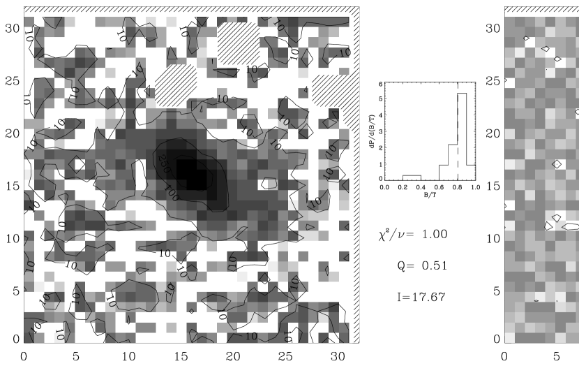
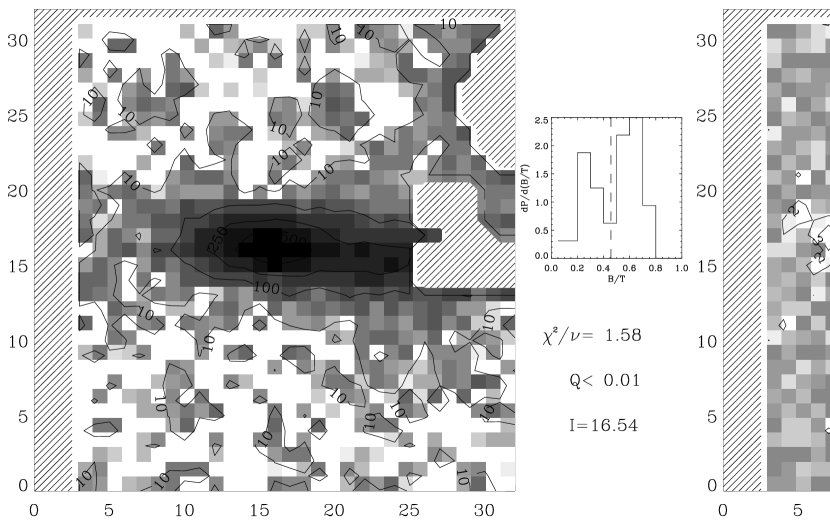
Figure 1: (cont.) Postage stamp images of three representative galaxies from our sample. The top row shows a galaxy that is fit very well by our procedure, the bottom row shows one that is poorly fit and the middle row shows a more typical result. The left hand column is the original $33\times 33$ pixel galaxy image with contours indicating the pixel value in ADUs. The right hand column is the residual image after subtracting the best fit model galaxy. Contours show the absolute value of the residual in units of $\sigma$, the rms uncertainty on each pixel value. Hatched regions contained contaminant galaxies and were removed by our automated cleaning procedure before fitting. (Where an entire row or column is hatched, the postage stamp image was recentered prior to fitting.) Between the original image and the residual maps we quote the value of $\chi^{2}$ per degree of freedom, $Q$ (the probability that a random fluctuation exceeds this value of $\chi^{2}$) and the I-band apparent magnitude. Also shown is a histogram of ${\rm d}P/{\rm d}({\rm B/T})$, the distribution of bulge-to-total ratios found from the Monte Carlo simulations described in the text, with a vertical dashed line indicating the best-fit B/T value for the original image.

The majority of galaxies (363 out of 626) are fit reasonably well by this procedure. We regard a galaxy as being reasonably well fit when $Q$, the probability that the measured value of $\chi^{2}$ is exceeded by random fluctuations, is greater than 5%. Not surprisingly though, many galaxies are not well fit. These typically show signs of strong morphological disturbance (perhaps due to a recent or imminent merger) or other inhomogeneities. Examples of well-fit and poorly-fit galaxies are given in Figure 1. Poorly-fit galaxies are easily identified by their large $\chi^{2}$ values and so may be excluded from further analysis if desired. It should be noted that a poor-fit does not indicate a failure of our fitting procedure per se, rather it signals that the galaxy is not well described by a combination of a spheroid and a disk. We choose to show results computed using the entire sample, regardless of how well a galaxy was fit, but we will comment on how our results change if badly fit galaxies are excluded from the analysis.

Errors on the fitted parameters could, in principle, be determined using a $\Delta\chi^{2}$ approach, but this would require mapping $\chi^{2}$ in the 12 dimensional parameter space of the fit — an exceedingly time consuming exercise — and, in any case, the errors are unlikely to be normally distributed given that the model is highly nonlinear in the parameters. We therefore adopt a Monte Carlo approach to error estimation. Using the best fitting model for each galaxy, we generate 30 realizations of that model, add random noise at the same level as in the real image, and mask out any pixels which were masked out in the original. We then find the best fitting parameters for each realization and take their distribution as indicative of the uncertainties in the actual fit. It should be noted that this is only a valid procedure if the original image is well fit by the model. In cases where this is not the case, there is no reason to expect the Monte Carlo distributions to give an estimate of the true errors. The B/T distributions for the three galaxies illustrated in Figure 1 are shown in that figure.

4 Results

4.1 Accuracy Checks

We begin by assessing the reliability of our procedure for recovering the true B/T ratio of a galaxy (assuming, of course, that real galaxies are well described by our model). Our Monte Carlo procedure for error estimation allows a determination of the accuracy of our technique. For each galaxy, the value of B/T input into the Monte Carlo simulations may be compared to the mean and standard deviation of the distribution of 30 recovered B/T values. Figure 2 gives the results of these accuracy tests. The left-hand panel shows the standard deviation of the recovered B/T ratio, as a function of the I-band apparent magnitude of the mock image. For bright galaxies ($m_{\rm I}~{}\hbox to0.0pt{$<$\hss}{\lower 4.30554pt\hbox{$\sim$}}16$), $\sigma_{\rm MC}$ is fairly small, typically less than about 0.1. However, for fainter galaxies, $\sigma_{\rm MC}$ increases very rapidly, resulting in rather poorly constrained B/T values. (In reality, $\sigma_{\rm MC}$ depends also upon the other parameters that describe the mock image, but the correlation with apparent magnitude is the most important.)

In the right-hand panel of Figure 2, we plot the mean value of B/T recovered from the Monte Carlo simulations against the true value for the mock image. The large solid circles indicate those images for which $\sigma_{\rm MC}\leq 0.1$. Evidently, for these galaxies the value of B/T is recovered accurately and without any strong systematic bias. The small dots show the results for all other galaxies. Now the scatter is much larger and, more importantly, there are systematic biases in the mean recovered B/T, such that very low and very high values are avoided. This effect is not surprising: the values of B/T for these faint galaxies are almost entirely unconstrained. (Note that the standard deviation for a completely uniform distribution of B/T is approximately 0.3.) As a result, the distribution of B/T from the Monte Carlo simulations becomes close to uniform, with the mean tending towards 0.5 as $\sigma_{\rm MC}$ increases. For the 90 galaxies in our sample with $m_{\rm I}\leq 16$, there is a tight correlation between $(B/T)_{\rm true}$ and the mean value recovered from the Monte Carlo simulations and it is this subsample that we will use below to compute luminosity functions. Unfortunately, its relatively small size limits the statistical accuracy of our estimates quite considerably.

Figure 2: Left-hand panel: the standard deviation, $\sigma_{\rm MC}$, of the distribution of recovered B/T ratios from 30 Monte Carlo realizations of a model galaxy image, as a function of the apparent I-band magnitude of the model image. Right-hand panel: the mean recovered B/T ratio from 30 Monte Carlo realizations of a model galaxy image plotted against the true B/T value. Large, filled circles show those galaxies for which $\sigma_{\rm MC}\leq 0.1$, while small open circles show all other galaxies.

To find the best fit solution we must choose initial values for the parameters to be fit and then use Powell’s algorithm to search for values producing a better fit. For parameters such as the position angles, disk inclination and spheroid/disk sizes we make initial guesses based on the image being fitted. Other parameters are initially assigned “typical” values. We have checked the effect of altering these initial values. For galaxies with $\sigma_{\rm MC}\leq 0.1$, the choice of initial value makes almost no difference to the recovered values of the parameters, indicating that our technique is finding the true minimum $\chi^{2}$. As $\sigma_{\rm MC}$ becomes larger, however, the recovered parameters begin to depend strongly upon the initial values chosen. For these images, the $\chi^{2}$ surface in the 12 dimensional parameter space does not possess an obvious minimum (i.e. it is very noisy). This is just another way of saying that the values of the fitted parameters for these faint images are highly uncertain.

Andredakis, Peletier & Balcells (1995) have demonstrated that the bulges of spiral galaxies are more accurately fit by an $r^{1/n}$, rather than by the more usual $r^{1/4}$, surface brightness profile, with values of $n$ ranging from around 1 to 6 (similar variations in $n$ are seen for elliptical galaxies; Bingelli & Cameron 1991; Caon, Capaccioli & D’Onofrio 1993). They show that the value of $n$ is strongly correlated with morphological type. Although our present data provide only rather poor constraints on the value of $n$ (due to limited angular resolution and signal-to-noise), we have nevertheless repeated the fitting procedure using $r^{1/n}$ profiles for the spheroids, treating $n$ as a free parameter. For galaxies where the B/T ratio is well determined, we find that there is a strong correlation between the B/T values obtained with $r^{1/4}$ and $r^{1/n}$ profiles, although inevitably some scatter is present. The disk and spheroid luminosity functions computed using B/T ratios from $r^{1/n}$ fits show no statistically significant difference from those using $r^{1/4}$ fits.

Finally, we remind the reader that our analysis makes use of a Gaussian PSF to mimic the effects of seeing in the data. A Gaussian accurately describes the core of the PSF measured from bright stars in the images. However, a profile consisting of a Gaussian core plus power-law wings provides a better match to many of the stellar profiles. (The variation of Gaussian and core components from night to night in the imaging data is not so well characterized, however, and this is why we make use of a simple Gaussian for our main analysis.) Fitting the images using such a profile (keeping the relative proportions of Gaussian and power-law wings fixed, but allowing the overall radial scale of the PSF to be a free parameter) results in small changes in the B/T ratio, typically significantly smaller than the error in the best fit value. Thus, the luminosity functions presented below are unaffected by the exact choice of PSF. However, it is clear that a good characterization of the PSF and its variation will be crucial to obtain accurate disk and spheroid luminosity functions from larger, higher quality datasets.

4.2 Luminosity Functions

Using the I$<16$ sample of approximately 90 galaxies for which we have good estimates of the B/T ratio we now proceed to estimate the disk and spheroid luminosity functions. Our aim here is to develop the techniques required for this measurement and demonstrate them using a particular dataset. Given the small size of the dataset we must expect that both statistical (due to the small number of galaxies) and systematic (due, for example, to the lack of rich clusters in the dataset) errors will be present. These issues are considered further in §5.

To determine the present-day luminosity functions, we need to apply k$+$e corrections to the galaxy luminosities. We use the type-dependent k$+$e corrections obtained by Gardner et al. (1997). Briefly, a set of model galaxy colors was computed using an updated version of the Bruzual & Charlot (1993) stellar population models with a range of star formation histories. The observed colors of each galaxy were matched to one of the models and that particular model was then used to extrapolate the observed galaxy luminosity to $z=0$. Note that our type-dependent k$+$e corrections are based on the total (i.e. disk plus spheroid) color of each galaxy. In principle, k$+$e corrections could be applied to each component separately if spheroid/disk decompositions were carried out in several bands. Given the uncertainties in our present estimates of B/T, we refrain from this degree of complexity in this analysis.

We use the stepwise maximum likelihood (SWML) estimator proposed by (Efstathiou, Ellis & Peterson, 1988, hereafter EEP) and also the parametric maximum likelihood method proposed by (Sandage, Tammann & Yahil, 1979, hereafter STY) to compute disk and spheroid luminosity functions. The detectability of a spheroid depends on both its apparent magnitude and the B/T ratio, and we must account for this in constructing the likelihood function. This leads us to define a two-dimensional function, $\Phi(M,B)$, such that $\Phi(M,B){\rm d}M{\rm d}B$ is the number of galaxies per unit volume with B/T ratio in the range $B$ to $B+{\rm d}B$ and spheroid absolute magnitude in the range $M$ to $M+{\rm d}M$ (with an equivalent definition for disks). The application of the maximum likelihood estimator to this function is discussed in detail in Appendix A. The normal luminosity function of spheroids is readily derived using $\phi(M)=\int_{0}^{1}\Phi(M,B){\rm d}B$ (and similarly for disks). For the STY method we must assume some parametric form for the luminosity function. We have tried fitting the disk and spheroid luminosity functions with a “Schechter$\otimes$exponential” form, namely $\Phi(M,B)=\phi(M)\exp(\beta B)$, where $\phi(M)$ is the normal Schechter function and $\beta$ is a parameter to be fit, motivated by the shape of the SWML estimate of these luminosity functions.

Figure 3: I-band luminosity functions. Triangles, circles and stars show the SWML estimates of the total, spheroid and disk luminosity functions respectively. Only galaxies brighter than $I=16$ have been used, k$+$e corrections have been applied to all galaxies, and distances have been calculated assuming $(\Omega_{0},\Lambda_{0})=(0.3,0.7)$. Errorbars are the sum in quadrature of the standard SWML errors and the variance in estimates of the luminosity function from 30 Monte Carlo realizations of the spheroid/disk decomposition procedure. The very heavy solid line shows the best fit Schechter function to the total luminosity function, while the inset shows the values of $\alpha$ and $M_{\star}$ for this fit, together with their 1 and $2\sigma$ error ellipses. The heavy and thin solid lines show the best-fit “Schechter$\otimes$exponential” functions to the spheroid and disk luminosity functions respectively, and confidence regions for $\alpha$ and $M_{\star}$ for these fits are given in the inset (the remaining parameter of the fits was $\beta=0.0\pm 0.37$ and $2.1\pm 0.37$ for spheroids and disks respectively).

Figure 3 shows the resulting I-band luminosity functions with distances computed assuming $(\Omega_{0},\Lambda_{0})=(0.3,0.7)$ and $H_{0}=100h$ km/s/Mpc. Triangles show the total luminosity function; circles and stars show the spheroid and disk luminosity functions separately. These SWML luminosity functions are normalized to the I-band number counts in the Sloan Digital Sky Survey using the procedure described in the Appendix. For the total luminosity function, we plot the standard SWML errorbars (obtained from the covariance matrix of the luminosity function as described by EEP), but for the spheroid and disk luminosity functions, the errorbars are the sum in quadrature of the standard SWML errors and the variance in the luminosity function estimated from the 30 Monte Carlo realizations of the spheroid/disk decomposition process. The errors from each source are of comparable magnitude (although the variance from the Monte Carlo realizations is the smaller of the two). The very heavy solid line shows the best-fitting Schechter function to the total luminosity function (determined using the STY method); the inset shows the values of $\alpha$ and $M_{\star}$ for this fit, together with their 1 and $2\sigma$ error contours. (The small sample size is reflected in rather large and correlated uncertainties in $M_{\star}$ and $\alpha$.) Heavy and thin solid lines show the best fit STY “Schechter$\otimes$exponential” luminosity function fits to the spheroid and disk luminosity functions respectively (with the corresponding confidence ellipses for $\alpha$ and $M_{\star}$ shown in the inset, and the values of $\beta$ given in the figure caption). A likelihood ratio test (Efstathiou, Ellis & Peterson, 1988) shows that the Schechter$\otimes$exponential luminosity function is not a particularly good fit to the data. With the present small dataset we have been unable to find a better functional form. This situation will be rectified with a larger dataset (assuming that some suitable functional form does actually exist).

The I-band luminosity functions of disks and spheroids are remarkably similar. The only significant difference is that the spheroid luminosity function is somewhat lower at faint magnitudes. However, given the small size of the present sample, this difference may not be robust. The luminosity densities in disks and spheroids obtained by integrating the SWML luminosity functions over the range of absolute magnitudes shown in Fig. 3 are $5.8\pm 0.8$ and $4.7\pm 0.7\times 10^{7}hL_{\odot}/\hbox{Mpc}^{3}$ respectively (where we have taken $M_{\odot}=4.14$ in the I-band; Cox 2000). In principle, we can use our Schechter$\otimes$exponential fits to estimate the total luminosity density, extrapolating to include the contribution from arbitrarily faint spheroids and disks. Doing so yields results which agree with the SWML estimates within the quoted errors, suggesting that our determination may have suitably converged. However, it must be kept in mind that the Schechter$\otimes$exponential form is not a particularly good fit to the current datasets.

Figure 4: Slices through the SWML estimate of the bi-variate luminosity function, $\Phi(M,B)$, for different absolute magnitudes, $M$, as indicated in the figure. Points were computed in bins of size $(\Delta M,\Delta B)=(0.48,0.33)$ and errors obtained as described by EEP. The upper panel shows the spheroid luminosity function, and the lower panel the disk luminosity function. The points without errorbars above the dotted line in each panel indicate the mean B/T (and D/T) for spheroids (and disks) in the corresponding absolute magnitude bins. Solid lines indicate the best-fit “Schechter$\otimes$exponential” parametric luminosity function for the $M_{\rm I}-5\log h=-19.82$ bin.

In Fig. 4, we show slices through the bi-variate luminosity function, $\Phi(M,B)$, at constant $M$ for several values of $M$ (as indicated in the figure, and in bins of width $\Delta M=0.48$). It is evident that $\Phi(M,B)$ is not independent of $B$ and that, in fact, it may not be separable into a simpler form $\Phi(M,B)=\phi(M)g(B)$. This is particularly noticeable for the spheroid luminosity function. Figure 4 shows that spheroid-dominated systems (i.e. B/T$>2/3$) are found only in the brightest spheroids, while disk-dominated systems (i.e. D/T$>2/3$) have disks with a much broader range of luminosities. This point is made more clearly in Fig. 5 where we show the spheroid luminosity function of spheroid-dominated systems and the disk luminosity function of disk-dominated systems. We find spheroid-dominated systems in abundance only brightwards of $M_{\rm I}-5\log h\approx-21$, but disk-dominated systems across the whole range of luminosities.

Figure 5: SWML estimates of the I-band luminosity functions of spheroids in spheroid-dominated galaxies (i.e. B$>2/3$; circles) and disks in disk-dominated galaxies (i.e. D/T$>2/3$; stars). The samples include 13 and 36 galaxies respectively. Errors are the sum in quadrature of the standard SWML errors and the variance found in luminosity functions estimated from 30 Monte Carlo realizations of the spheroid/disk decomposition procedure.

4.3 The stellar mass in disks and spheroids

The stellar mass associated with the luminosity of each galaxy is easily obtained by a similar procedure to that employed to calculate the k-corrections (namely fitting their BVIK colors to a set of template galaxies). We use these estimates to construct the stellar mass functions of spheroids and disks in the local Universe and thereby estimate the total mass content in each component. The method that we adopt is the same that Cole et al. (2001) used to measure the total stellar mass density in the Universe from a combination of 2dFGRS and 2MASS data. Cole et al. (2001) found the stellar mass density in units of the critical density to be $\Omega_{\rm stars}=0.0016\pm 0.00024h^{-1}$ or $\Omega_{\rm stars}=0.0029\pm 0.00043h^{-1}$, depending on whether a Kennicutt (1983) or a Salpeter (1955) stellar initial mass function (IMF) was assumed. (Both estimates include the effects of dust on galaxy luminosities as described by Cole et al. 2001.) We normalize our stellar mass functions by requiring them to produce the same number density of galaxies more massive than $M_{*}$ as the Cole et al. (2001) stellar mass function. The total stellar mass density inferred from our ${\rm I}<18$ sample is then $\Omega_{\rm stars}=0.0009\pm 0.00007h^{-1}$ or $\Omega_{\rm stars}=0.0017\pm 0.00012h^{-1}$ for the same two IMFs respectively and the same prescription for dust-extinction. Errors on the stellar mass density were found by summing in quadrature the error from each individual bin in the SWML mass function, together with the error in the overall normalization. Our estimates include contributions from galaxies with stellar masses greater than $10^{9}h^{-2}M_{\odot}$ below which the SWML stellar mass function is not well determined. We can check our result using the STY stellar mass function. For this, we fit a Schechter function convolved with a Gaussian of width $0.1$ in $\log_{10}M_{\rm stars}$ to account for the scatter in the relation between stellar mass and I-band absolute magnitude. We find that our estimates of $\Omega_{\rm stars}$ using the SWML and STY mass functions agree within the errors, suggesting that the result has already converged to sufficient accuracy. Our estimates, however, are lower than those of Cole et al. (2001), a reflection of the flatter faint end slope of our mass functions which may well be due to the small size of our sample.

For our ${\rm I}<16$ sample, for which the bulge-to-total ratio is well measured, we find a slightly higher total stellar mass density of $\Omega_{\rm stars}=0.0012\pm 0.00014h^{-1}$ for the Kennicutt (1983) IMF. Splitting into spheroidal and disk components, we find $\Omega_{\rm stars,spheroids}=0.00039\pm 0.00006h^{-1}$ and $\Omega_{\rm stars,disks}=0.00051\pm 0.00008h^{-1}$ for this same IMF. (Note that with the SWML method the stellar mass densities of disks and spheroids are not guaranteed to sum to give the total stellar mass density.) If, instead, we assume a Salpeter IMF, the ratio of disk to spheroid stellar mass densities increases slightly from 1.31 to 1.37, but this change is negligible given the current errors in these quantities. Although the small size of our sample is clearly a significant limitation, this initial result suggests that spheroids and disks contribute about equally to the stellar mass density of the Universe. The techniques developed in this paper, when applied to a much larger dataset, should allow their contributions to be more accurately determined.

5 Discussion

We have presented a detailed method to determine the bulge-to-total ratios of galaxies by fitting to two-dimensional photometry, and have applied this technique to determine the I-band bulge-to-total luminosity ratios of a sample of approximately 600 galaxies brighter than I$=18$ with spectroscopic redshifts. Our approach is designed to work with realistic galaxy images, dealing automatically with contamination by nearby objects, a varying PSF and small changes in the background from image to image. A crucial part of the fitting procedure is a Monte Carlo determination of the errors on the fitted parameters, an approach which is favored since it is fast and automatically accounts for the highly non-linear nature of the model parameters. For the current sample of galaxies, around 60% are well fit by a combination of an exponential disk and an $r^{1/4}$-law spheroid. Those that are not well fit frequently show signs of morphological disturbance. We find that bulge-to-total ratios are determined accurately (i.e. with errors of around $10\%$) only for galaxies brighter than I$\approx 16$.

For the 90 galaxies brighter than I$=16$ in this sample we measure the B/T ratio with reasonable accuracy. We have used the resulting disk/spheroid decomposition of these bright galaxies to construct separate luminosity functions for disks and spheroids. We find no significant differences between them when considered purely in terms of luminosity, although the statistical uncertainties associated with the small sample size make the detection of any differences difficult. However, when we consider the bi-variate distributions of luminosity and bulge-to-total or disk-to-total light, we find that spheroid dominated systems (B/T$>2/3$) only occur for the brightest spheroids, while disk-dominated systems (D/T$>2/3$) occur for a much broader range of disk luminosities.

The relative contributions of disks and spheroids to the total stellar mass density in the Universe is a very important constraint on theories of galaxy formation which attempt to describe the assembly of galaxies as a function of time. We find, perhaps surprisingly, that the disks and spheroids in our sample contribute almost equally to the stellar mass density today (in a ratio of $1.3\pm 0.2$). Since the stellar populations in disks are generally younger than those in spheroids, it is an interesting coincidence that the total stellar mass in the two kinds of structural components should be so similar at the present time.

Schechter & Dressler (1987) reached a similar conclusion to ours using a photometric comparison technique to estimate the B-band bulge-to-disk ratios of galaxies. While this technique may not be as accurate as our own on a galaxy-by-galaxy basis, it should provide a good estimate of the total contribution of each component to the stellar mass density. It is therefore reassuring that our results agree well with those of Schechter & Dressler (1987). A different result was obtained by Fukugita, Hogan & Peebles (1998), who derived a ratio of disk to spheroid stellar mass density of $0.33\pm 0.23$. Although they found comparable B-band luminosity density in spheroids and disks, they adopted a spheroid mass-to-light ratio around four times greater than that for disks, resulting in spheroids making a significantly greater contribution to the stellar mass density. While we use a more accurate technique for converting from luminosity to stellar mass (a technique which could be improved further if B/T ratios were measured for each galaxy in several bands), the small size of our sample limits the accuracy of our results. In particular, our sample may not contain enough rich clusters which are known to contain higher fractions of spheroid dominated galaxies than the field (e.g. Dressler 1980) and this could introduce a small bias in our results.

Clearly the greatest limitation of this work is the small size of the sample of galaxies for which accurate disk/spheroid decompositions can be performed. Fortunately, this problem should be remedied in the near future with the advent of high quality, large area photometric surveys such as that being carried out by the SDSS project.

Appendix A. Estimators for Spheroid and Disk Luminosity Functions

The traditional $1/V_{\rm max}$ estimator is trivially adapted to the case of disk and spheroid luminosity functions. The estimator is applied just as in the case of the standard luminosity function, except that the total luminosity of the galaxy (i.e. disk plus spheroid luminosity) is used to compute $V_{\rm max}$, since it is this total luminosity that determines the volume within which the galaxy could have been detected.

The maximum likelihood estimator of Efstathiou, Ellis & Peterson (1988, hereafter EEP) is also easily generalized to the case of spheroid and disk luminosity functions. Consider the case of the spheroid luminosity function (the same arguments apply to disks). As noted earlier, the detectability of a spheroid depends upon both its absolute magnitude, $M$, and on the bulge-to-total ratio which we denote by $B$ in this Appendix. We begin therefore by defining a two-dimensional function, $\Phi(M,B)$, such that $\Phi(M,B){\rm d}M{\rm d}B$ is the number of galaxies with bulge-to-total ratio in the range $B$ to $B+{\rm d}B$ and spheroid absolute magnitude $M$ to $M+{\rm d}M$ per unit volume. The normal luminosity function of spheroids is easily recovered using $\phi(M)=\int_{0}^{1}\Phi(M,B){\rm d}B$. The probability that galaxy $i$ with spheroid magnitude $M_{i}$ and bulge-to-total ratio $B_{i}$ is seen in a magnitude limited survey is

$$p_{i}\propto\Phi(M_{i},B_{i})\left/\int_{0}^{1}\int_{-\infty}^{M^{\prime}_{\rm lim}(z_{i},B)}\Phi(M,B){\rm d}M{\rm d}B\right.,$$ (4)

where $M^{\prime}_{\rm lim}(z_{i},B)=M_{\rm lim}(z_{i})-2.5\log_{10}B$ and $M_{\rm lim}(z_{i})$ is the limiting absolute magnitude of the survey at redshift $z_{i}$. The use of $M^{\prime}_{\rm lim}$ is necessary since arbitrarily faint spheroids will make it into the survey provided that they have a sufficiently low bulge-to-total ratio (corresponding to sufficiently bright disks).

From this definition we can construct the usual likelihood function

$$\ln{\mathcal{L}}=\sum_{i=1}^{N}\ln\Phi(M_{i},B_{i})-\sum_{i=1}^{N}\ln\left\{\int_{0}^{1}\int_{-\infty}^{M^{\prime}_{\rm lim}(z_{i},B)}\Phi(M,B){\rm d}M{\rm d}B\right\}+\hbox{const},$$ (5)

where $N$ is the total number of galaxies. There are now two ways to proceed. In the first we assume a simple parametric form for $\Phi(M,B)$ and maximize the likelihood with respect to the parameters. This is analogous to fitting a Schechter function (Schechter, 1976) to the normal luminosity function (e.g. Sandage, Tammann & Yahil 1979). A simple parametric form which we have tried to fit our data is

$$\Phi(M,B)=\phi(M)\exp(\beta B),$$ (6)

where $\phi(M)$ is the usual Schechter function and $\beta$ is a parameter to be estimated from the fit. With this method, the likelihood function of eqn. (5) can be evaluated for each value of the three parameters $\alpha$, $\beta$ and $M_{\star}$, and hence the parameter values which maximize the likelihood are readily obtained.

The second approach involves splitting $\Phi(M,B)$ into bins in $M$ and $B$ and treating each as a parameter. This is equivalent to the SWML method of EEP for estimating the standard luminosity function.

We represent $\Phi(M,B)$ as follows:

$$\Phi(M,B)=\Phi_{k,h},\left\{\begin{array}[]{ll}M_{k}-\Delta M/2<M<M_{k}+\Delta M/2,&k=1,\ldots,N_{p}\\ B_{h}-\Delta B/2<B<B_{h}+\Delta B/2,&h=1,\ldots,N_{q}.\end{array}\right.$$ (7)

The likelihood function may then be written as

$$\ln{\mathcal{L}}=\sum_{i=1}^{N}W(M_{i}-M_{k},B_{i}-B_{h})\ln\Phi_{k,h}-\sum_{i=1}^{N}\ln\left\{\sum_{h=1}^{N_{q}}\sum_{k=1}^{N_{p}}\Phi_{k,h}\Delta M\Delta BH[M_{k},B_{h},M_{\rm lim}(z_{i})]\right\}+\hbox{const},$$ (8)

where

$$W_{k,h}(M_{i},B_{i})=\left\{\begin{array}[]{ll}1&\hbox{if }M_{k}-\Delta M/2<M_{i}<M_{k}+\Delta M/2,\hbox{ and }B_{h}-\Delta B/2<B_{i}<B_{h}+\Delta B/2,\\ 0&\hbox{otherwise}\end{array}\right.$$ (9)

and

$$H[M_{k},B_{h},M_{\rm lim}(z_{i})]={1\over\Delta M\Delta B}\int_{B_{h}-\Delta B/2}^{B_{h}+\Delta B/2}\int_{M_{k}-\Delta M/2}^{M_{k}+\Delta M/2}Q(M,B){\rm d}M{\rm d}B,$$ (10)

where $Q(M,B)=0$ if $M>M_{\rm lim}(z_{i})-2.5\log_{10}B$ and $Q(M,B)=1$ otherwise. Since only the shape of the luminosity function is constrained by the above likelihood function, we introduce an additional constraint, $g=\sum_{k}\sum_{h}\Phi_{k,h}(L_{k,h}/L_{\rm f})^{\beta}\Delta M\Delta B-1=0$, where $L_{k,h}$ is the total luminosity of a galaxy with spheroid magnitude $M_{k}$ and bulge-to-total ratio $B_{h}$ and $L_{\rm f}$ is a fiducial luminosity (which we will take to be that corresponding to $M_{\rm I}-5\log h=-20.5$), using a Lagrangian multiplier $\lambda$ as did EEP. Maximizing $\ln{\mathcal{L}}^{\prime}=\ln{\mathcal{L}}+\lambda g$ then yields

$$\Phi_{k,h}={\sum_{i=1}^{N}W(M_{i}-M_{k},B_{i}-B_{k})\over\sum_{i=1}^{N}H[M_{k},B_{h},M_{\rm lim}(z_{i})]/\sum_{l=1}^{N_{p}}\sum_{m=1}^{N_{q}}\Phi_{l,m}H[M_{l},B_{m},M_{\rm lim}(z_{i})]}$$ (11)

which are easily solved with an iterative procedure. The covariance matrix for the parameters is obtained in a manner entirely analogous to that outlined by EEP.

Normalization of the maximum likelihood luminosity function can be achieved using the actual redshift data as described by Loveday et al. (1992), but using $M^{\prime}_{\rm lim}$ in the selection function to account for the effects of the bulge-to-total ratio. A better approach is to normalize by performing a least squares fit to the number counts of galaxies from a wide area survey. The cumulative number count to apparent magnitude $m$ is given by

$$n(m)=\int_{0}^{\infty}\int_{0}^{1}\int_{-\infty}^{M^{\prime}_{\rm lim}}\Phi(m-D(z)-K(z)-2.5\log_{10}B,B){{\rm d}V\over{\rm d}z}{\rm d}M{\rm d}B{\rm d}z,$$ (12)

where $D(z)$ and $K(z)$ are the distance modulus and k$+$e correction respectively at redshift $z$, which we can compute from the SWML estimate of $\Phi$.

References

- Abraham et al. (1996) Abraham R. G., van den Bergh S., Glazebrook K., Ellis R. S., Santiago B. X., Surma P., Griffiths R. E., 1996, ApJS, 107, 1