The mode trapping properties of full DA white dwarf evolutionary models

An adiabatic, non-radial pulsation study of a 0.563 M_⊙DA white dwarf model is presented on the basis of new evolutionary calculations performed in a self-consistent way with the predictions of time dependent element diffusion, nuclear burning and the history of the white dwarf progenitor. Emphasis is placed on the role played by the internal chemical stratification of these new models in the behaviour of the eigenmodes, and the expectations for the full g-spectrum of periods. The implications for the mode trapping properties are discussed at length. In this regard, we find that, for high periods, the viability of mode trapping as a mode selection mechanism is markedly weaker for our models, as compared with the situation in which the hydrogen-helium transition region is treated assuming equilibrium diffusion in the trace element approximation.

1 Introduction

Since photometric variations were detected in the white dwarf HL Tau 76 (Landolt 1968), astronomers have been observing multimode pulsations in an increasing number of these objects. Of particular interest are the variable white dwarfs characterized by hydrogen-rich atmospheres. These variable stars, known in the literature as ZZ Ceti or DAV stars, constitute the most numerous group amongst degenerate pulsators. Other class of pulsating white dwarfs are the DBV, with helium-rich atmospheres, and the pre-white dwarfs DOVs and PNNVs, which show spectroscopically pronounced carbon, oxygen and helium features (for reviews of the topic, see Winget 1988 and Kepler & Bradley 1995). In particular, ZZ Ceti stars are found in a narrow interval of effective temperature ($T_{\rm eff}$) ranging from 12500 K $\gtrsim T_{\rm eff}\gtrsim$ 10700 K. Their brightness variations, which reach up to 0.30 magnitudes, are interpreted as being caused by spheroidal, non-radial g(gravity)-modes of low degree ($\ell\leq 2$) and low and intermediate overtones $k$ (the number of zeros in the radial eigenfunction), with periods ($P_{k}$) between 2 and 20 minutes. Radial modes, although found overstables in a number of theoretical studies of pulsating DA white dwarfs (see, e.g. Saio et al. 1983), have been discarded as the cause of variability in such stars. This is so because the periods involved are shorter than 10 seconds. Observationally these high-frequency signatures have not been detected thus far. With regard to the mechanism that drives pulsations, the $\kappa-\gamma$ mechanism is the traditionally accepted one (Dolez & Vauclair 1981 and Winget et al. 1982). Nonetheless, Brickhill (1991) proposed the convective driving mechanism as being responsible for the overstability of g-modes in DAVs (see also Goldreich & Wu 1999). Although both mechanisms predict roughly the observed blue edge of the instability strip, none of them are capable to yield the red edge, where pulsations of DA white dwarfs seemingly cease in a very abrupt way (Kanaan 1996).

A longstanding problem in the study of pulsating DA white dwarfs is to find the reason of why only a very reduced number of modes are observed, as compared with the richness of modes predicted by theoretical studies. Indeed, it has been long suspected that some filtering mechanism must be acting quite efficiently. The explanation commonly proposed is that of “mode trapping” phenomenon (Winget et al. 1981; Brassard et al. 1992a; Bradley 1996). According to this mechanism, those modes (the trapped ones) having a local radial wavelength comparable with the thickness of the hydrogen envelope, require low kinetic energy to reach observable amplitudes. Then, most of the observed periods should correspond to trapped modes. Nevertheless, in a recent asteroseismological study of the ZZ Ceti star G117-B15A (Bradley 1998), the observed period of 215 s, which has the larger amplitude in the power spectrum, does not correspond to the trapped mode predicted by the best fitting model.

The exploration of these very important aspects requires the construction of detailed DA white dwarf evolutionary models, particularly regarding the treatment of the chemical abundance distribution. Work in this direction has recently begun to be undertaken. In fact, Althaus et al. (2002) have carried out full evolutionary calculations which take into account time dependent element diffusion, nuclear burning and the history of the white dwarf progenitor in a self-consistent way. Specifically, these authors have followed the evolution of an initially 3 M_⊙stellar model all the way from the stages of hydrogen and helium burning in the core through the thermally pulsing and mass loss phases till the white dwarf state. Althaus et al. (2002) find that the shape of the Ledoux term (an important ingredient in the computation of the Brunt-Väisälä frequency; see Brassard et al. 1991, 1992ab) is markedly different from that found in previous detailed studies of white dwarf pulsations. This is due partly to the effect of smoothness in the chemical abundance distribution caused by element diffusion, which gives rise to less pronounced peaks in the Ledoux term. This, in turn, leads to a substantially weaker mode trapping effect, as it has recently been found by Córsico et al. (2001). These authors have presented the first results regarding the trapping properties of the Althaus et al. (2002) evolutionary models.

The present work is designed to explore at some length the pulsation properties of the Althaus et al. (2002) evolutionary models and to compare our predictions with those of others investigators. In addition, the work is intended to bring some more insight to the phenomenon of mode trapping in the frame of these new evolutionary models. In particular, we shall restrict ourselves to analyse the same stellar model as that studied in Córsico et al. (2001). Specifically, the model, which belongs to the ZZ Ceti instability strip, is analyzed in the frame of linear, non-radial stellar pulsations in the adiabatic approximation. Emphasis will be placed on assessing the role played by the internal chemical stratification in the behaviour of eigenmodes, and the expectations for the full spectrum of periods. Specifically, we shall explore the effects of the chemical interfaces on the kinetic energy distribution of the modes and their ability to modify the properties of the g-mode propagation throughout the star interior. We want to mention that, because of the high computational demands involved in the evolutionary calculations in which white dwarf cooling is assessed in a self-consistent way with element diffusion and the history of the pre-white dwarf, we are forced to restrict our attention to only one value for the stellar mass.

The article is organized as follows. In Sect. 2, we briefly describe our evolutionary and pulsational codes. In this section we also discuss some aspects concerning the evolutionary properties of our models. In Sect. 3 we present in detail the pulsation results. Finally, Sect. 4 is devoted to summarizing our findings.

2 Details of computations

Our selected ZZ Ceti model on which the pulsational results are based has been calculated by means of an evolutionary code developed by us at La Plata Observatory. The code, which is based on a detailed and up-to-date physical description, has enabled us to compute the white dwarf evolution in a self-consistent way with the predictions of time dependent element diffusion, nuclear burning and the history of the white dwarf progenitor. The constitutive physics includes: new OPAL radiative opacities for different metallicities, conductive opacities, neutrino emission rates and a detailed equation of state. In addition, a network of 30 thermonuclear reaction rates for hydrogen burning (proton-proton chain and CNO bi-cycle) and helium burning has been considered. Nuclear reaction rates are taken from Caughlan & Fowler (1988) and Angulo et al. (1999) for the ${}^{12}{\rm C}(\alpha,\gamma)^{16}{\rm O}$ reaction rate. This rate is about twice as large as that of Caughlan & Fowler (1988). Abundance changes resulting from nuclear burning are computed by means of a standard implicit method of integration. In particular, we follow the evolution of the chemical species ¹H, ³He, ⁴He, ⁷Li, ⁷Be, ¹²C, ¹³C, ¹⁴N, ¹⁵N, ¹⁶O, ¹⁷O, ¹⁸O and ¹⁹F. Convection has been treated following the standard mixing length theory (Böhm-Vitense 1958) with the mixing-length to pressure scale height parameter of $\alpha=$1.5. The Schwarzschild criterium was used to determine the boundaries of convective regions. Overshooting and semi-convection were not considered. Finally, the various processes relevant for element diffusion have also been taken into account. Specifically, we considered the gravitational settling, and the chemical and thermal diffusion of nuclear species ¹H, ³He, ⁴He, ¹²C, ¹⁴N and ¹⁶O. Element diffusion is based on the treatment for multicomponent gases developed by Burgers (1969). It is important to note that by using this treatment of diffusion we are avoiding the widely used trace element approximation (see Tassoul et al. 1990). After computing the change of abundances by effect of diffusion, they are evolved according to the requirements of nuclear reactions and convective mixing. Radiative opacities are calculated for metallicities consistent with the diffusion predictions. This is done during the white dwarf regime in which gravitational settling leads to metal-depleted outer layers. In particular, the metallicity is taken as two times the abundance of CNO elements. For more details about this and other computational details we refer the reader to Althaus et al. (2002) and Althaus et al. (2001).

We started the evolutionary calculations from a 3 M_⊙  stellar model at the zero-age main sequence. The adopted initial metallicity is $Z$= 0.02 and the initial abundance by mass of hydrogen and helium are, respectively, $X_{\rm H}$= 0.705 and $X_{\rm He}$= 0.275. Evolution has been computed at constant stellar mass all the way from the stages of hydrogen and helium burning in the core up to the tip of the asymptotic giant branch where helium thermal pulses occur. After experiencing 11 thermal pulses, the model is forced to evolve towards the white dwarf state by invoking strong mass loss episodes. The adopted mass loss rate was $\approx 10^{-4}$ M_⊙yr^-1 and it was applied to each stellar model as evolution proceeded. After the convergence of each new stellar model, the total stellar mass is reduced according to the time step used and the mesh points are appropriately adjusted. As a result of mass loss episodes, a white dwarf remnant of 0.563 M_⊙  is obtained. The evolution of this remnant is pursued through the stage of planetary nebulae nucleus till the domain of the ZZ Ceti stars on the white dwarf cooling branch.

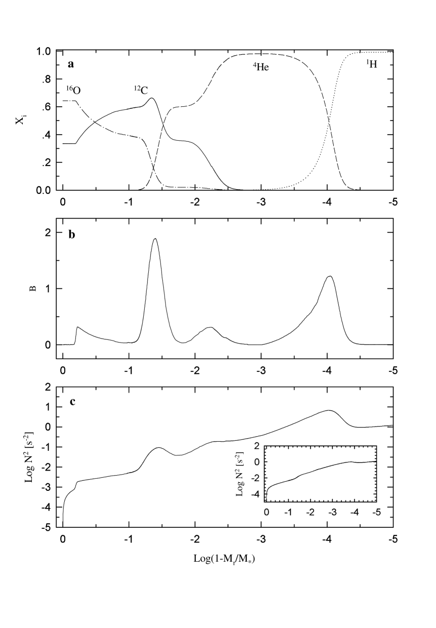
Figure 1: Panel a: The chemical abundance distribution of our stellar model for hydrogen (dotted line), helium (dashed line), carbon (solid line) and oxygen (dot-dashed line). Panel b: the Ledoux term, $B$. Panel c: the logarithm of the squared of the Brunt-Väisälä frequency ($N^{2}$). In the inset of this panel, the logarithm of the squared of the Brunt-Väisälä frequency computed neglecting the term $B$ is depicted. Note that the imprints of the chemical transition zones in the functional form of $N^{2}$ are not completely eliminated, in particular at the helium-carbon-oxygen and hydrogen-helium interfaces. The stellar mass of the white dwarf model is 0.563 ${\rm M_{\odot}}$ and the effective temperature is $\approx$ 12000K. Quantities are shown in terms of the outer mass fraction.

As well known, the shape of the composition transition zones plays an important role in the pulsational properties of DAV white dwarfs. In this sense, an important aspect of these calculations concerns the evolution of the chemical abundance during the white dwarf regime. In particular, element diffusion makes near discontinuities in the chemical profile at the start of the cooling branch be considerably smoothed out by the time the ZZ Ceti domain is reached (see Althaus et al. 2002). The chemical profile throughout the interior of our selected white dwarf model is depicted in the upper panel of Fig. 1. Only the most abundant isotopes are shown. In particular, the inner carbon-oxygen core emerges from the convective helium core burning and from the subsequent stages in which the helium-burning shell propagates outwards. Note also the flat profile of the carbon and oxygen distribution towards the centre. This is a result of the chemical rehomogenization of the innermost zone of the star due to Rayleigh-Taylor instability (see Althaus et al. 2002). Above the carbon-oxygen interior there is a shell rich in both carbon ($\approx$ 35%) and helium ($\approx$ 60%), and an overlying layer consisting of nearly pure helium of mass 0.003 M_⊙. The presence of carbon in the helium-rich region below the pure helium layer is a result of the short-lived convective mixing which has driven the carbon-rich zone upwards during the peak of the last helium pulse on the asymptotic giant branch. We want to mention that the total helium content within the star once helium shell burning is eventually extinguished amounts to 0.014 M_⊙  and that the mass of hydrogen that is left at the start of the cooling branch is about $1.5\times 10^{-4}$ M_⊙, which is reduced to $7\times 10^{-5}$ M_⊙  due to the interplay of residual nuclear burning and element diffusion by the time the ZZ Ceti domain is reached. Finally, we note that the inner carbon-oxygen profile of our models is somewhat different from that of Salaris et al. (1997). In particular, we find that the size of the carbon-oxygen core is smaller than that found by Salaris et al. (1997) with the consequent result that the drop in the oxygen abundance above the core is not so pronounced as in the case found by these authors. We suspect that this different behaviour could be a result of a different treatment of the convective boundary during the core helium burning.

For the pulsation analysis we have employed the code described in Córsico & Benvenuto (2002). We refer the reader to that paper for details. Here we shall describe briefly our strategy of calculation and mention the pulsation quantities computed that are relevant in this study. The pulsational code is based on the general Newton-Raphson technique (like the Henyey method employed in stellar evolution studies). The code solves the differential equations governing the linear, non-radial stellar pulsations in the adiabatic approximation (see Unno et al. 1989 for details of their derivation). The boundary conditions at the stellar centre and surface are those given by Osaki & Hansen (1973) (see Unno et al. 1989 for details). Following previous studies of white dwarf pulsations, the normalization condition adopted is $\delta r/r=1$ at the stellar surface. After selecting a starting stellar model we choose a convenient period window and the interval of interest in $T_{\rm eff}$. The evolutionary code computes the white dwarf cooling until the hot edge of the $T_{\rm eff}$-interval is reached. Then, the program calls the set of pulsation routines to begin the scan for modes. In order to obtain the first approximation to the eigenfunctions and the eigenvalue of a mode we have applied the method of the discriminant (Unno et al. 1989). Specifically, we adopt the potential boundary condition (at the surface) as the discriminant function (see Córsico & Benvenuto 2002). When a mode is found, the code generates an approximate solution which is iteratively improved to convergence (of the eigenvalue and the eigenfunctions simultaneously) and then stored. This procedure is repeated until the period interval is covered. Then, the evolutionary code generates the next stellar model and calls pulsation routines again. Now, the previously stored modes are taken as initial approximation to the modes of the present stellar model and iterated to convergence.

For each computed mode we obtain the eigenperiod $P_{k}$ ($P_{k}=2\pi/\sigma_{k}$, being $\sigma_{k}$ the eigenfrequency) and the dimensionless eigenfunctions $y_{1},\cdots,y_{4}$ (see Unno et al. 1989 for their definition). With these eigenfunctions and the dimensionless eigenvalue $\omega_{k}^{2}=\sigma^{2}_{k}(GM_{*}/R_{*}^{3})^{-1}$ we compute for each mode considered the oscillation kinetic energy, $(E_{\rm kin})_{k}$, given by:

$$(E_{\rm kin})_{k}=\frac{1}{2}(GM_{*}R_{*}^{2})\omega_{k}^{2}\int_{0}^{1}x^{2}\rho\left[x^{2}y_{1}^{2}+x^{2}\frac{\ell(\ell+1)}{(C_{1}\omega_{k}^{2})^{2}}y_{2}^{2}\right]dx,$$ (1)

and the first order rotation splitting coefficient, $C_{\ell,k}$,

$$C_{\ell,k}=\frac{(GM_{*}R_{*}^{2})}{2(E_{\rm kin})_{k}}\int_{0}^{1}\frac{x^{2}\rho}{C_{1}}\left[2x^{2}y_{1}y_{2}+\frac{x^{2}}{C_{1}\omega_{k}^{2}}y_{2}^{2}\right]dx,$$ (2)

where $M_{*}$ and $R_{*}$ are the stellar mass and the stellar radius respectively, $G$ is the gravitation constant, $C_{1}=(r/R_{*})^{3}(M_{*}/M_{r})$ and $x=r/R_{*}$. In addition, we compute the weight functions, $WF$, and the variational period, $P_{k}^{\rm V}$, as given by Kawaler et al. (1985). Finally, for each model computed we derive the asymptotic spacing of periods, $\Delta P_{\rm A}$, given by (Tassoul 1980; Tassoul et al. 1990):

$$\Delta P_{\rm A}=\frac{P_{0}}{\sqrt{\ell(\ell+1)}},$$ (3)

and $P_{0}$ is defined as

$$P_{0}=2\pi^{2}\ \left[\int_{0}^{x_{2}}\frac{N}{x}dx\right]^{-1},$$ (4)

where $x_{2}$ correspond to the location of the base of the outer convection zone. The Brunt-Väisälä frequency ($N$), a fundamental quantity of white dwarf pulsations, is computed employing the “modified Ledoux” treatment. This treatment explicitly accounts for the contribution to $N^{2}$ from any change in composition in the interior of model (the zones of chemical transition) by means of the Ledoux term $B$ (see Brassard et al. 1991). We want to mention that we have also employed a numerical differentiation scheme for computing $N^{2}$ directly from its definition. We found that this scheme yields the same results as those derived from the modified Ledoux treatment.

As mentioned, for the pulsation analysis in this study we have selected a white dwarf model representative of the ZZ Ceti instability band. Specifically, we have picked out a 0.563 ${\rm M_{\odot}}$ model at $T_{\rm eff}\approx$ 12000 K. In Table 1 we show the main characteristics of our template model. In the interests of comparison, the same quantities corresponding to a similar model of P. Bradley (2002) (private communication) are shown. The Brunt-Väisälä frequency and the Ledoux term ($B$) corresponding to our template model are shown in the middle and bottom panels of Fig. 1 in terms of the outer mass fraction. Note the particular shape of $B$, which is a

Table 1.

	Our template	Bradley’s model
	model
$M_{*}/{\rm M_{\odot}}$	0.563	0.560
$T_{\rm eff}$ [K]	11996	12050
$\log(L_{*}$/L${}_{\odot})$	-2.458	-2.462
$\log(R_{*}$/R${}_{\odot})$	-1.864	-1.866
$\log(M_{\rm H}/M_{*})$	-3.905	-3.824
$\log(M_{\rm He}/M_{*})$	-1.604	-1.824
$\log(\rho_{c})$ [g cm-3]	6.469	6.466
$\log(T_{c})$ [106 K]	7.086	7.087

direct consequence of the chemical profile. In turn, the features of $B$ are reflected in the Brunt-Väisälä frequency. As a result of element diffusion, the chemical profiles of our evolutionary models are very smooth in the interfaces (see upper panel of Fig. 1), and this explains the presence of extended tails in the shape of $B$. Also, note that our model is characterized by a chemical interface in which three ionic species in appreciable abundances coexists: helium, carbon and oxygen (see early in this section). This transition region gives two contributions to $B$, one of them of relatively great magnitude, placed at $\log q\sim-1.4$, and the other, more external and of very low height at $\log q\sim-2.2$. As a last remark, the contribution of the hydrogen-helium interface to $B$ is less than that corresponding to the helium-carbon-oxygen transition. Note that the contributions from the Ledoux term are translated into smooth bumps on $N^{2}$. The characteristics of $B$ and $N^{2}$ as predicted by our models are markedly different from those found in previous studies in which the white dwarf evolution is treated in a simplified way, particularly regarding the chemical abundance distribution in the outer layers (e.g., Tassoul et al. 1990; Brassard et al. 1991, 1992ab; Bradley 1996). For more details see Althaus et al. (2002).

3 Results

For our template model we have computed g-modes with $\ell=1,2$ and $3$ (we do this because geometric cancellation effects grow progressively for larger $\ell$ in non-radial oscillations; see Dziembowski 1977), with periods in the range of 50 s $\lesssim P_{k}\lesssim$ 1300 s. Let us quote that for mode calculations we have employed up to 5000 mesh points. For all of our pulsation calculations, the relative difference between $P_{k}$ and $P_{k}^{\rm V}$ remains lower than $10^{-3}$. This gives an indication of the accuracy of our calculations.

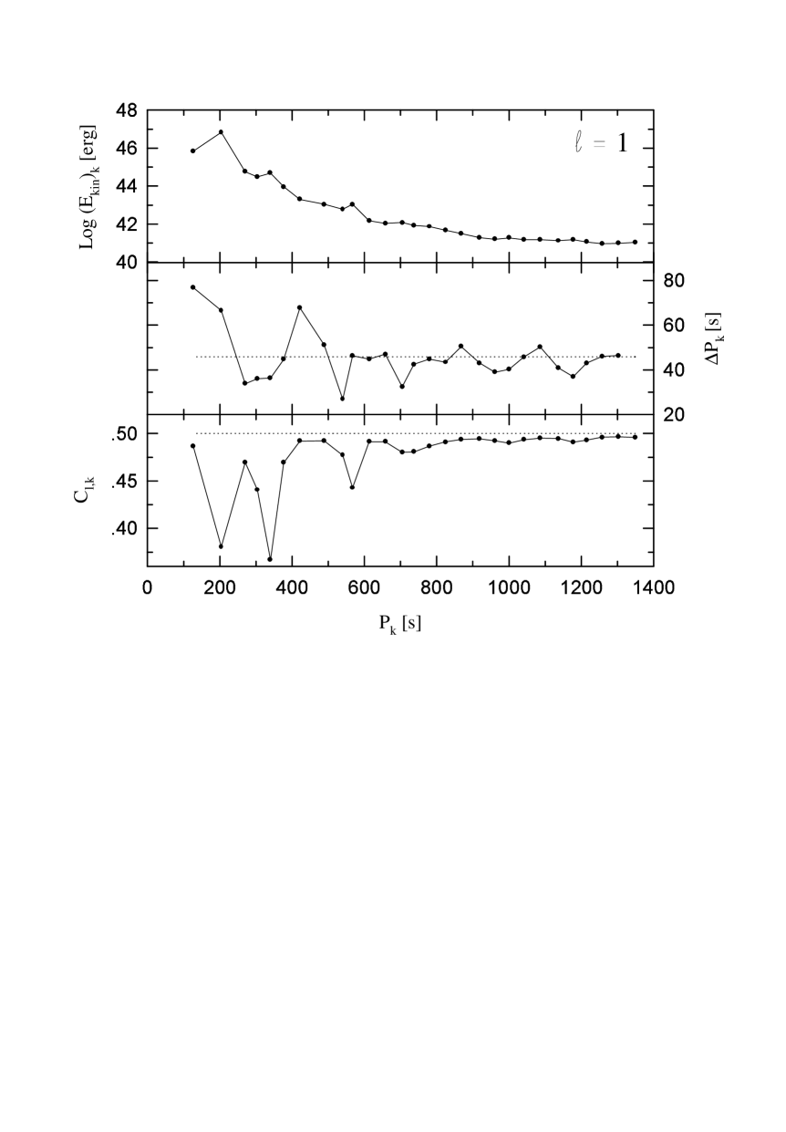
Figure 2: The logarithm of the oscillation kinetic energy, forward period spacing and first order rotation splitting coefficient (upper, middle and lower panels, respectively) for modes with $\ell=1$ as a function of computed periods. Dotted lines show the asymptotic behaviour for $\Delta P_{k}$ and $C_{\ell,k}$. The values of $(E_{\rm kin})_{k}$ correspond to the normalization $y_{1}=\delta r/r=1$ at $r=R_{*}$.

We begin by examining Figs. 2 to 4, the upper panels of which show the logarithm of the oscillation kinetic energy of modes with, respectively, $\ell=1,2$ and $3$ in terms of computed periods. Middle panels depict the values for the forward period spacing $\Delta P_{k}$ ($\equiv P_{k+1}-P_{k}$) together with the asymptotic value $\Delta P_{\rm A}$ as given by dotted lines . Finally, in the bottom panel of these figures we depict the $C_{\ell,k}$ values as well as the asymptotic values (dotted lines) that these coefficients adopt for high overtones, that is $C_{\ell,k}\approx 1/\ell(\ell+1)$ (Brickhill 1975). An inspection of plots reveals some interesting characteristics. To begin with, the quantities plotted exhibit two clearly different trends. Indeed, for $P_{k}\gtrsim 500-600$ s and irrespective of the value of $\ell$, the distribution of oscillation kinetic energy is quite smooth. Note that the $\log(E_{\rm kin})_{k}$ values of adjacent modes are quite similar, which is in contrast with the situation found for lower periods. On the other hand, the period spacing diagrams show appreciable departures of $\Delta P_{k}$ from the asymptotic prediction (Eq. 3) for $P_{k}\lesssim 500-600$ s. As well known, this is due mostly to the presence of chemical abundance transitions in DA white dwarfs. In contrast, for higher periods the $\Delta P_{k}$ of the modes tend to $\Delta P_{\rm A}$. Also, note that the $C_{\ell,k}$ values tend to the asymptotic value for $P_{k}\gtrsim 500-600$ s.

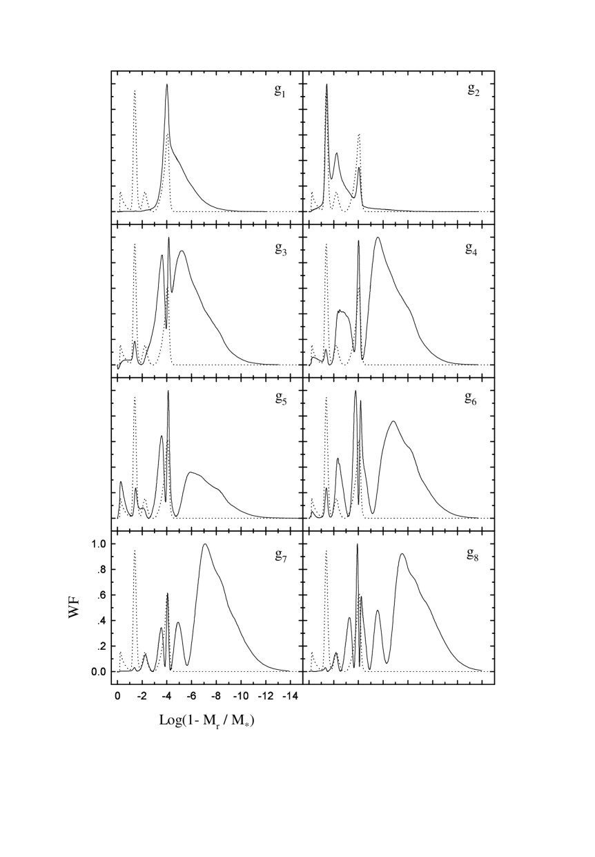
Figure 5: The normalized weight function (solid lines) in terms of the outer mass fraction, for modes g₁ to g₈ with $\ell=1$. In the interests of comparison, dotted lines depict the run of the Ledoux term (arbitrary units).

An important aspect of the present study is related to the mode trapping and confinement properties of our models. For the present analysis we shall employ the weight functions, $WF$. We elect $WF$ because this function gives the relative contribution of the different regions in the star to the period formation (Kawaler et al. 1985; Brassard et al. 1992ab). We want to mention that we have also carefully examined the density of kinetic energy (the integrand of Eq. 1) for each computed mode. For our purposes here, this quantity gives us basically the same information that provided by $WF$. We show in Fig. 5 to 7 the $WF$ for all of the computed modes corresponding to $\ell=1$. In addition, we include in each plot of these figures the Ledoux term in arbitrary units (dotted lines) in order to make easier the location of the chemical transition regions of the model. In the interests of a proper interpretation of these figures, we suggest the reader to see also Fig. 2. For low periods, a variety of behaviour is encountered. For instance, the g₁ mode is characterized by a $WF$ corresponding to the well known mode trapping phenomenon, that is, g₁ is formed in the very outer layers irrespective of the details of the deeper chemical profile, as previously reported by previous studies (see Brassard et al. 1992ab). In contrast, it is the helium-carbon-oxygen transition that mostly contributes to the formation of the g₂ mode, whilst the hydrogen-helium transition plays a minor role. This mode would be representative of the “confined modes” according to Brassard et al. (1992ab). $WF$ for modes g₃ and g₄ is qualitatively similar to that of g₁, except that they are not exclusively formed in the hydrogen-rich envelope, but also in the helium-carbon-oxygen interface. On the other hand, the high-density zone underlying the helium-carbon-oxygen transition plays a major role in the formation of mode g₅. From Eq. (1) is clear that the $(E_{\rm kin})_{k}$ values are proportional to the integral of the squared eigenfunctions, weighted by $\rho$. As a result, the g₅ mode is characterized by a high oscillation kinetic energy value (see Fig. 2). Note that the helium-carbon-oxygen transition region also contributes to the formation of modes g₆ and g₁₀. The g₁₀ mode is particularly interesting, because it is formed over a wide range of the stellar interior, thus being also a high kinetic energy mode. The $WF$s corresponding to remaining modes do not differ appreciably amongst them. They exhibit contributions mainly from the outer layers of the model, though they also show small amplitudes in deeper regions. Note that for all of the modes shown in Figs. 5 to 7 there is a strong contribution to $WF$s from the hydrogen-helium transition region. This indicate that, as found in previous studies, this chemical interface plays a fundamental role in the period formation of modes. We want to mention that we have elected for this analysis the dipolar modes ($\ell=1$) for brevity; the results for $\ell=2,3$ are qualitatively similar to those of $\ell=1$.

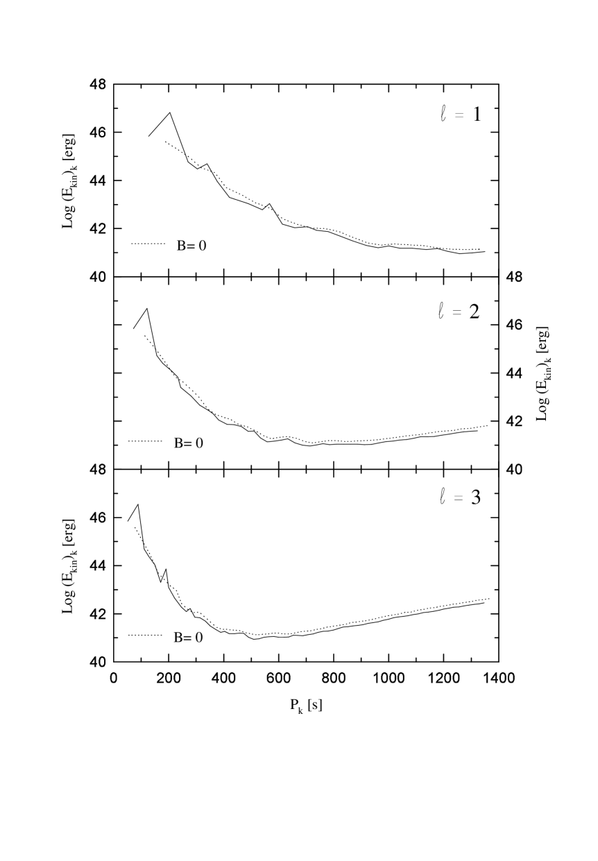
Figure 8: The logarithm of the oscillation kinetic energy for modes with $\ell=1$, $\ell=2$ and $\ell=3$ (upper, middle and lower panel, respectively), as a function of computed periods. In the interests of clarity, symbols corresponding to eigenmodes have been omitted. Solid lines correspond to our template model, and dotted lines correspond to the “homogeneous” model in which $B=$ 0.

From the analysis performed above based on the weight functions, we can clearly appreciate that for $P_{k}\gtrsim 500-600$ s the outer layer of the model appreciably contribute to the $WF$s. This is expected, because, as well known, $g$-modes in white dwarfs are envelope modes. As mentioned, the $WF$s of high order modes are very similar, indicating that these modes have essentially the same characteristics. At this point, we could, in principle, classify these modes either like trapped or partially trapped in the outer envelope or like “normal” modes (in the terminology of Brassard et al. 1992), that is, without enhanced or diminished oscillation kinetic energies as in the case of eigenmodes corresponding to chemically homogeneous stellar models. In fact, the curves $\log(E_{\rm kin})_{k}-P_{k}$ depicted in Figs. 2 to 4, in particular for periods exceeding $500-600$ s, strongly resemble the kinetic energy distribution corresponding to a model in which there no exist chemical interfaces. With the aim of solving such an ambiguity, we have performed pulsation calculations arbitrarily setting $B=0$ in the computation of the Brunt-Väisälä frequency. As mentioned, the modified Ledoux treatment employed in the computation of the Brunt-Väisälä frequency bears explicitly the effect from changes in chemical composition by means of the Ledoux term $B$. So, by forcing $B=0$ the effects of the chemical transitions are strongly minimized (but not completely eliminated; see inset of Fig. 1c) on the whole pulsational pattern. In this way we obtain an approximate chemically homogeneous white dwarf model (see Brassard et al. 1992b for a similar numerical experiment). The oscillation kinetic energy values resulting for this simulated “homogeneous” model are shown in Fig. 8 with dotted lines. In the interests of a comparison, we show the results corresponding to our (full) template model with solid lines. It is clear from the figure that the distribution of $(E_{\rm kin})_{k}$ values for both sets of computations (and for each value of $\ell$) is very similar in the region of long periods. However, note that the curves corresponding to the modified model are shifted to higher energies (by $\approx 0.2$ dex) as compared with the situation of the full model. We have carefully compared the $WF$ for each mode of the full model with the corresponding mode of the “homogeneous” model (i.e. modes which have closest period values although generally for different radial order $k$). We found that, for modes with periods exceeding $\approx 600$ s, the $WF$s are almost identical in both cases at the regions above the hydrogen-helium transition. However, below this interface the $WF$s corresponding to the “homogeneous” model show larger amplitudes as compared with the case of the full model. Thus, we can conclude that for the full model, all the modes corresponding to the long period region of the pulsational spectrum must be considered as partially trapped in the hydrogen-rich envelope. In others words, the chemical distribution at the hydrogen-helium transition has noticeable effect on each mode, but this effect is the same for all modes. This conclusion is reinforced by the fact that the first order rotation splitting coefficients ($C_{\ell,k}$) for the full model adopt higher values as compared with those corresponding to the “homogeneous” model (not shown here for brevity), thus lying nearest to the asymptotic prediction. As found by Brassard et al. (1992ab), it is an additional characteristic feature of trapped modes in the hydrogen-rich outer region of white dwarfs.

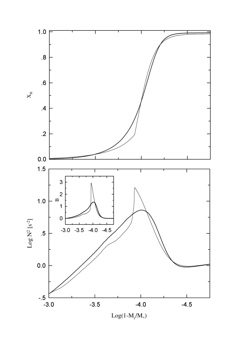
Figure 9: Upper panel: hydrogen abundance distribution at the hydrogen-helium interface as given by multicomponent, non-equilibrium diffusion (solid line) and diffusive equilibrium in the trace element approximation (thin line). Lower panel: the logarithm of the squared Brunt-Väisälä frequency for the both treatment of diffusion mentioned above. The inset shows the prediction for the Ledoux term. For details, see text.

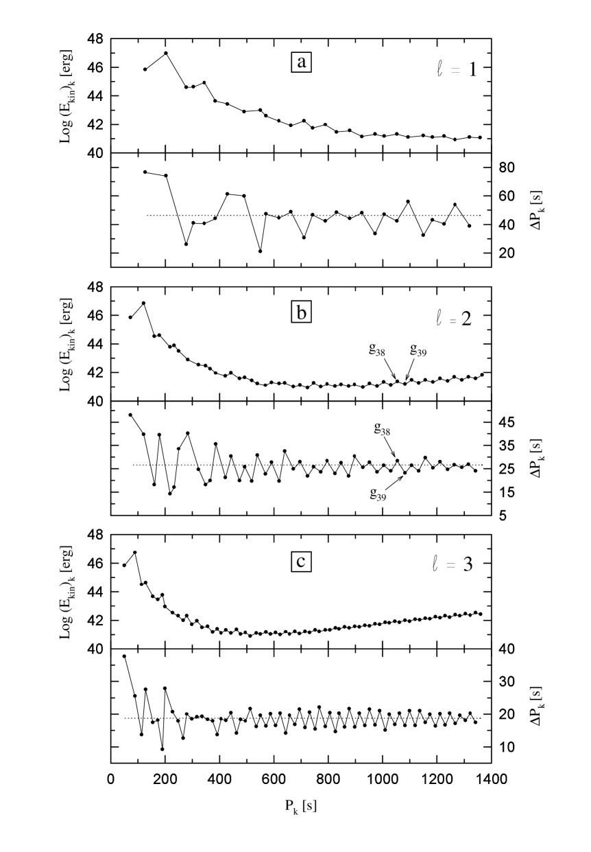
Figure 10: The logarithm of the oscillation kinetic energy (upper panel) and period spacing (lower panel) for $\ell=1$ (figure a), $\ell=2$ (figure b) and $\ell=3$ (figure c) in terms of the computed periods, for the case of diffusive equilibrium in the trace element approach. As found in previous studies, this approximation gives rise to a kinetic energy pattern and spacing of consecutive periods in which trapping signatures are clearly noted. This is in contrast to the prediction of time dependent element diffusion given in Figs. 2 to 4.

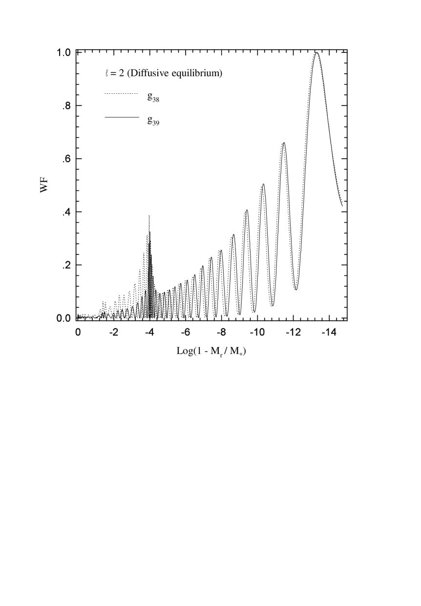
Figure 11: The normalized weight function for modes g₃₈ and g₃₉ with $\ell=2$ corresponding to the stellar model in which the hydrogen-helium chemical transition has been treated in the diffusive equilibrium and trace element approximation. Note the lower amplitude of $WF$ below the hydrogen-helium transition for mode with $k$= 39, which corresponds to a trapped one in the hydrogen envelope.

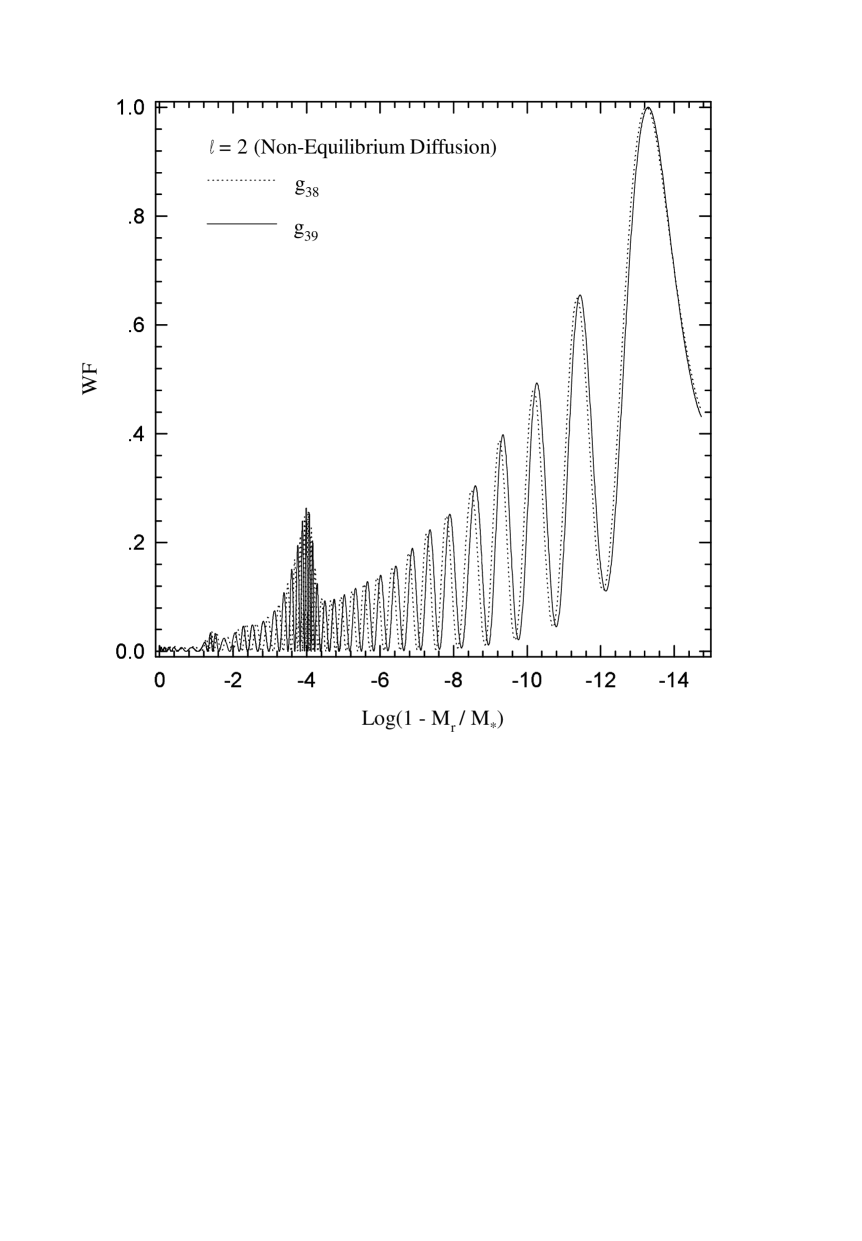
Figure 12: Same of Fig. 11, but for the case in which the hydrogen-helium chemical transition has been computed assuming time dependent element diffusion.

An important finding of this work is the effect of chemical abundance distribution resulting from time dependent diffusion on the mode trapping properties in DA white dwarfs. In fact, as shown in Fig. 2 to 4, for periods exceeding $\approx 500-600$ s, the distribution of $(E_{\rm kin})_{k}$ is smooth, and $\Delta P_{k}$ values tend to the asymptotic value. This is quite different from that found in previous studies. Our calculations reveal that the capability of mode filtering due to mode trapping effects virtually vanish for high periods when account is made of white dwarf models with diffusively evolving chemical stratifications (see Córsico et al. 2001). In order to make a detailed comparison of the predictions of our models with those found in previous studies we have carried out additional pulsational calculations by assuming diffusive equilibrium in the trace element approximation at the hydrogen-helium interface (see Tassoul et al. 1990). This treatment has been commonly invoked in most of the pulsation studies to model the composition transition regions. The resulting hydrogen chemical profile and the corresponding Ledoux term and Brunt-Väisälä frequency $N$ are shown in Fig. 9, together with the predictions of time dependent element diffusion. The trace element assumption leads to an abrupt change in the slope of the chemical profile which is responsible for the pronounced peak in the Brunt-Väisälä frequency at $\log(1-M_{r}/M_{*})\approx-4$. As can be clearly seen in Fig. 10 for $\ell=1$ to 3, the diffusive equilibrium in the trace element approximation gives rise to an oscillation kinetic energy spectrum and period spacing distribution that are substantially different from those given by the full treatment of diffusion (see Figs. 2 to 4), particularly for high periods. The most outstanding feature depicted by Fig. 10 is the trapping signatures exhibited by certain modes both in the $\log(E_{\rm kin})_{k}$ and $\Delta P_{k}$ values. This is in agreement with other previous results (see Brassard et al. 1992b, particularly their figures 20a and 21a for the case of $M_{\rm H}=10^{-4}M_{*}$). As well known, trapped modes correspond to those modes which are characterized by minima in their oscillation kinetic energy values and local minima in the period spacing having the same $k$-value or differing by 1. For the purpose of illustration, we compare in Fig. 11 and 12 the predictions of equilibrium diffusion in the trace element approximation and time-dependent element diffusion, respectively, for $WF$ corresponding to the modes g₃₈ and g₃₉ with $\ell=2$. Clearly, in the case of diffusive equilibrium in the trace element approximation, mode g₃₉ corresponds to a trapped mode characterized by small values of the weight function below the hydrogen-helium transition, as compared with the adjacent, non-trapped mode g₃₈. By contrast, such modes show very similar amplitudes of their $WF$ when account is taken of a full diffusion treatment to model the composition transition regions (see Fig. 12). We would also like to comment on the fact that the diffusive equilibrium condition is far from being reached at the bottom of the hydrogen envelope of our model. In Althaus et al. (2002) we argued that the situation of diffusive equilibrium in the deep layers of a DAV white dwarf is not an appropriate one for describing the shape of the chemical composition at the hydrogen-helium transition zone. In fact, during the ZZ Ceti stage time-dependent diffusion modifies the spatial distribution of the elements, particularly at the chemical interfaces (see also Iben & MacDonald 1985). In addition, for the case of thick hydrogen envelopes, we have recently found that under the assumption of diffusive equilibrium, a white dwarf does not evolve along the cooling branch, but rather it experiences a hydrogen thermonuclear shell flash (see Córsico et al. 2002). This is so because if diffusion had plenty of time to evolve to an equilibrium situation then the tail of the hydrogen distribution would have been able to reach hot enough layers to be ignited in a flash fashion.

To place some of the results of the foregoing paragraph in a more quantitative basis, we list in Tables 2 and 3 the values for $P_{k}$, $\Delta P_{k}$ and $\log(E_{\rm kin})_{k}$ for modes corresponding to $\ell=$ 1 and $\ell=$ 2, in the case of equilibrium diffusion and time dependent element diffusion. In Table 2, the “m” corresponds to minima, and “M” stands for maxima. We have labeled the minima of $\Delta P_{k}$ and the minima and maxima of $\log(E_{\rm kin})_{k}$, in correspondence with Fig. 10. Note that for the case with $\ell=1$ there is a direct correlation (indicated by arrows) between minima in $\log(E_{\rm kin})_{k}$ and $\Delta P_{k-1}$ for most of high order modes, whereas for the case with $\ell=$ 2 this correspondence is between minima in $\log(E_{\rm kin})_{k}$ and $\Delta P_{k}$. The modes with minima in kinetic energy are classified as trapped (T) ones. In contrast to the case of equilibrium diffusion, the results corresponding to the time dependent element diffusion treatment do not show clear minima or maxima in kinetic energy, as can be appreciated in Figs. 2 to 4 and Table 3. We have compared the periods of our model with those kindly provided by Bradley corresponding to his 0.560 $M_{\odot}$ white dwarf model, and we find that our periods are typically 6 % shorter. In part, this difference is due to the somewhat smaller mass of the Bradley’s model and the different input physics characterizing both stellar models.

Table 2. Pulsation properties for $\ell=1,2$ modes

corresponding to the case of equilibrium diffusion.

$\ell=1$						$\ell=2$
$\Delta P_{\rm A}=$ 46.26 s						$\Delta P_{\rm A}=$ 26.71 s
$k$	$P_{k}$		$\Delta P_{k}$		$\log(E_{\rm kin})_{k}$	$k$	$P_{k}$		$\Delta P_{k}$		$\log(E_{\rm kin})_{k}$
	[s]		[s]		[erg]		[s]		[s]		[erg]
1	126.99	T	76.38		45.84 m	1	73.39	T	48.02		45.84 m
2	203.37		73.91		46.97 M	2	121.40		39.77		46.85 M
3	277.28	T	26.02 m	$\leftarrow$	44.60 m	3	161.17	T	18.11 m	$\leftarrow$	44.52 m
4	303.30		40.79		44.61 m	4	179.28		39.51		44.61 M
5	344.09		40.65		44.93 M	5	218.80	T	14.17 m	$\leftarrow$	43.77 m
6	384.75		44.00		43.62 m	6	232.97		17.06		43.89 M
7	428.75		61.25		43.43	7	250.03		33.50		43.49
8	490.00	T	59.93		42.90 m	8	283.53		40.06		42.89
9	549.93		21.12 m	$\swarrow$	42.99 M	9	323.59	T	24.67		42.53 m
10	571.05		47.22		42.59	10	348.26		18.24 m	$\swarrow$	42.48 M
11	618.27		44.54 m		42.23	11	366.50		19.88		42.27
12	662.81	T	48.65	$\nwarrow$	41.91 m	12	386.39		35.55		41.95
13	711.46		30.69 m		42.24 M	13	421.94	T	21.12 m	$\leftarrow$	41.76 m
14	742.15	T	46.66	$\nwarrow$	41.75 m	14	443.06		30.37		41.96 M
15	788.81		42.28 m		41.98 M	15	473.43	T	19.88 m	$\leftarrow$	41.58 m
16	831.09	T	48.51	$\nwarrow$	41.48 m	16	493.32		25.75		41.66 M
17	879.60		43.99 m		41.55 M	17	519.06		19.59 m		41.45
18	923.59	T	48.15	$\nwarrow$	41.16 m	18	538.65		30.84		41.21
19	971.75		33.31 m		41.31 M	19	569.49	T	22.68 m	$\leftarrow$	41.10 m
20	1005.05	T	47.02	$\nwarrow$	41.16 m	20	592.18		27.64		41.29 M
21	1052.07		42.38 m		41.32 M	21	619.82		19.68 m		41.22
22	1094.45	T	55.95	$\nwarrow$	41.10 m	22	639.51		32.53		41.26 M
23	1150.40		32.44 m		41.22 M	23	672.04	T	24.88 m	$\leftarrow$	41.00 m
24	1182.83	T	43.15	$\nwarrow$	41.09 m	24	696.92		27.97		41.12 M
25	1225.98		40.36 m		41.16 M	25	724.89	T	21.88 m	$\leftarrow$	40.93 m
26	1266.34	T	53.93	$\nwarrow$	40.93 m	26	746.77		25.83		41.25 M
27	1320.27		38.87 m		41.11 M	27	772.60	T	23.68 m	$\leftarrow$	41.01 m
$\ldots$	$\ldots$		$\ldots$		$\ldots$	28	796.28		28.33		41.18 M
$\ldots$	$\ldots$		$\ldots$		$\ldots$	29	824.61	T	22.94 m	$\leftarrow$	41.03 m
$\ldots$	$\ldots$		$\ldots$		$\ldots$	30	847.55		27.53		41.17 M
$\ldots$	$\ldots$		$\ldots$		$\ldots$	31	875.08	T	21.89 m	$\leftarrow$	41.04 m
$\ldots$	$\ldots$		$\ldots$		$\ldots$	32	896.97		30.30		41.14 M
$\ldots$	$\ldots$		$\ldots$		$\ldots$	33	927.27	T	25.47 m	$\leftarrow$	40.98 m
$\ldots$	$\ldots$		$\ldots$		$\ldots$	34	952.74		27.78		41.22 M
$\ldots$	$\ldots$		$\ldots$		$\ldots$	35	980.52	T	23.58 m	$\leftarrow$	41.06 m
$\ldots$	$\ldots$		$\ldots$		$\ldots$	36	1004.10		26.44		41.32 M
$\ldots$	$\ldots$		$\ldots$		$\ldots$	37	1030.54	T	23.93 m	$\leftarrow$	41.12 m
$\ldots$	$\ldots$		$\ldots$		$\ldots$	38	1054.46		28.40		41.35 M
$\ldots$	$\ldots$		$\ldots$		$\ldots$	39	1082.87	T	23.20 m	$\leftarrow$	41.18 m
$\ldots$	$\ldots$		$\ldots$		$\ldots$	40	1106.07		26.52		41.48 M
$\ldots$	$\ldots$		$\ldots$		$\ldots$	41	1132.58	T	23.99 m	$\leftarrow$	41.27 m
$\ldots$	$\ldots$		$\ldots$		$\ldots$	42	1156.57		29.72		41.46 M
$\ldots$	$\ldots$		$\ldots$		$\ldots$	43	1186.29	T	25.32 m	$\leftarrow$	41.32 m
$\ldots$	$\ldots$		$\ldots$		$\ldots$	44	1211.61		27.85		41.57 M
$\ldots$	$\ldots$		$\ldots$		$\ldots$	45	1239.47	T	24.74 m	$\leftarrow$	41.41 m
$\ldots$	$\ldots$		$\ldots$		$\ldots$	46	1264.20		26.62		41.68 M
$\ldots$	$\ldots$		$\ldots$		$\ldots$	47	1290.82	T	25.45 m	$\leftarrow$	41.48 m
$\ldots$	$\ldots$		$\ldots$		$\ldots$	48	1316.27		26.83		41.70 M

Table 3. Same as Table 2, but for the case of time-dependent

element diffusion.

$\ell=1$				$\ell=2$
$\Delta P_{\rm A}=$ 45.83 s				$\Delta P_{\rm A}=$ 26.30 s
$k$	$P_{k}$	$\Delta P_{k}$	$\log(E_{\rm kin})_{k}$	$k$	$P_{k}$	$\Delta P_{k}$	$\log(E_{\rm kin})_{k}$
	[s]	[s]	[erg]		[s]	[s]	[erg]
1	126.98	76.87	45.84	1	72.14	49.34	45.84
2	203.85	66.57	46.83	2	121.48	34.89	46.69
3	270.43	33.77	44.77	3	156.38	21.63	44.72
4	304.19	35.98	44.48	4	178.00	32.08	44.41
5	340.17	36.30	44.69	5	210.09	23.30	44.10
6	376.47	44.67	43.97	6	233.39	10.74	43.84
7	421.13	67.75	43.30	7	244.12	36.72	43.40
8	488.88	51.08	43.04	8	280.85	31.47	43.05
9	539.95	26.84	42.78	9	312.31	33.28	42.67
10	566.80	46.27	43.04	10	345.59	16.62	42.44
11	613.06	44.76	42.18	11	362.21	19.97	42.30
12	657.83	46.99	42.03	12	382.18	30.40	42.05
13	704.82	32.45	42.08	13	412.58	25.26	41.87
14	737.27	42.44	41.93	14	437.84	26.30	41.86
15	779.71	44.78	41.88	15	464.14	24.63	41.78
16	824.49	43.42	41.68	16	488.77	21.89	41.58
17	867.91	50.43	41.50	17	510.66	22.90	41.59
18	918.34	43.07	41.23	18	533.56	24.96	41.30
19	961.42	38.91	41.20	19	558.53	27.11	41.14
20	1000.33	40.24	41.28	20	585.64	24.25	41.17
21	1040.57	45.71	41.19	21	609.89	22.92	41.21
22	1086.28	50.32	41.19	22	632.80	26.05	41.27
23	1136.60	40.88	41.13	23	658.86	28.13	41.09
24	1177.48	36.91	41.17	24	686.98	27.00	41.00
25	1214.40	42.99	41.06	25	713.98	23.95	40.97
26	1257.38	46.02	40.96	26	737.94	22.71	41.01
27	1303.40	46.39	40.99	27	760.64	24.69	41.07
$\ldots$	$\ldots$	$\ldots$	$\ldots$	28	785.33	25.47	41.02
$\ldots$	$\ldots$	$\ldots$	$\ldots$	29	810.80	25.67	41.05
$\ldots$	$\ldots$	$\ldots$	$\ldots$	30	836.47	24.62	41.04
$\ldots$	$\ldots$	$\ldots$	$\ldots$	31	861.09	24.42	41.04
$\ldots$	$\ldots$	$\ldots$	$\ldots$	32	885.51	25.09	41.05
$\ldots$	$\ldots$	$\ldots$	$\ldots$	33	910.60	27.09	41.02
$\ldots$	$\ldots$	$\ldots$	$\ldots$	34	937.69	27.41	41.03
$\ldots$	$\ldots$	$\ldots$	$\ldots$	35	965.11	25.02	41.09
$\ldots$	$\ldots$	$\ldots$	$\ldots$	36	990.12	24.63	41.15
$\ldots$	$\ldots$	$\ldots$	$\ldots$	37	1014.75	24.66	41.18
$\ldots$	$\ldots$	$\ldots$	$\ldots$	38	1039.41	25.64	41.21
$\ldots$	$\ldots$	$\ldots$	$\ldots$	39	1065.05	26.07	41.23
$\ldots$	$\ldots$	$\ldots$	$\ldots$	40	1091.12	24.20	41.29
$\ldots$	$\ldots$	$\ldots$	$\ldots$	41	1115.32	24.33	41.35
$\ldots$	$\ldots$	$\ldots$	$\ldots$	42	1139.66	26.34	41.36
$\ldots$	$\ldots$	$\ldots$	$\ldots$	43	1166.00	27.19	41.37
$\ldots$	$\ldots$	$\ldots$	$\ldots$	44	1193.19	26.48	41.42
$\ldots$	$\ldots$	$\ldots$	$\ldots$	45	1219.67	26.20	41.46
$\ldots$	$\ldots$	$\ldots$	$\ldots$	46	1245.87	25.35	41.52
$\ldots$	$\ldots$	$\ldots$	$\ldots$	47	1271.22	25.13	41.56
$\ldots$	$\ldots$	$\ldots$	$\ldots$	48	1296.35	25.98	41.58

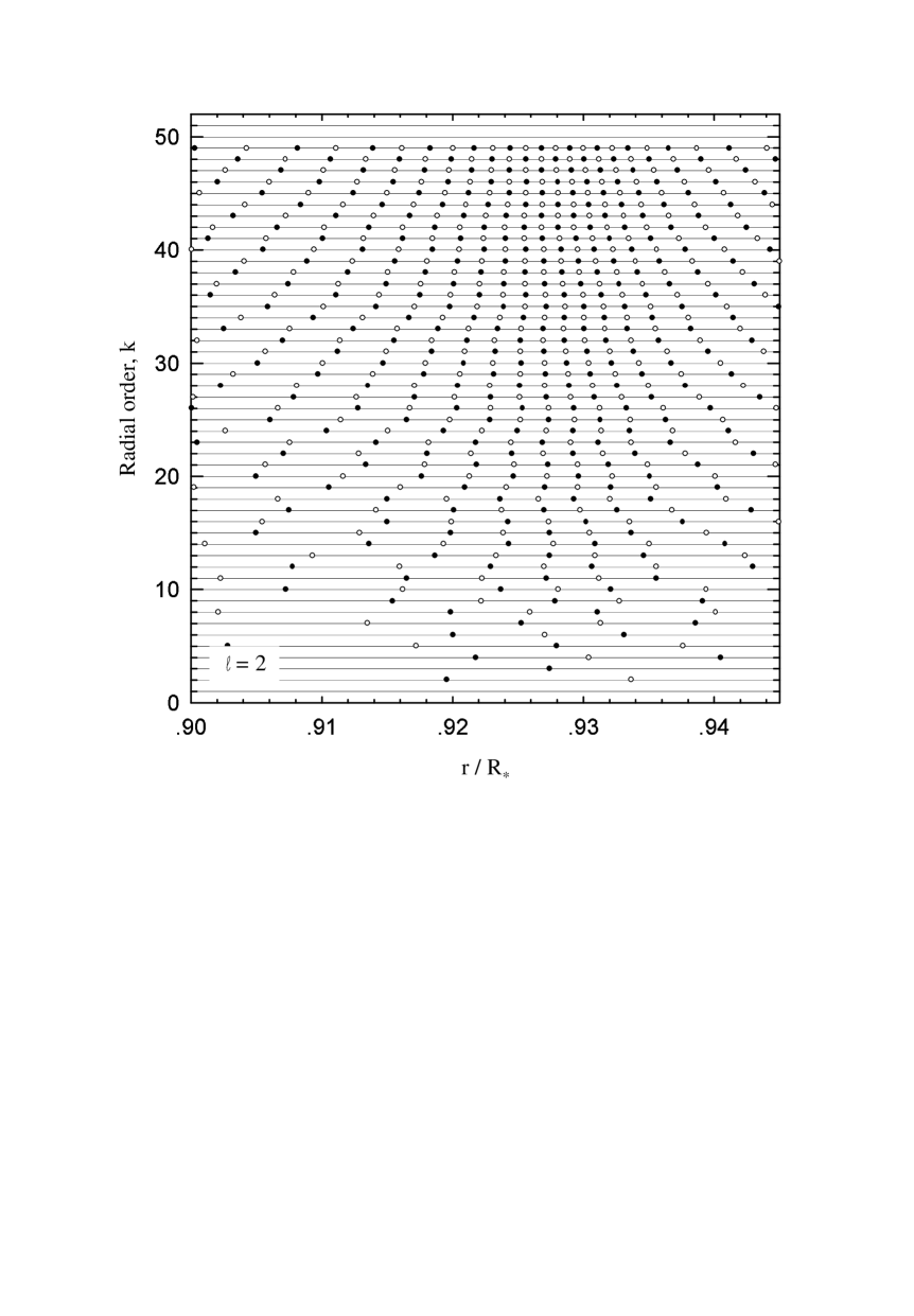
Figure 14: Same as Fig. 13, but for the case of chemical profiles resulting from time dependent element diffusion. See text for details.

On the basis of our results, we claim that the treatment of the chemical profile at the chemical transitions is a key ingredient in the computation of the g-spectrum. This is particularly true regarding the mode trapping properties, which are considerably altered when a physically sound treatment of the chemical evolution is incorporated in such calculations. This conclusion is valid at least for massive hydrogen envelopes as predicted by our full evolutionary calculations. To get a deeper insight into these aspects, we examine the node distribution of the eigenfunctions (Figs. 13 and 14). According to Brassard et al. (1992a), this is an useful diagnostic for mode trapping. Here, a mode is trapped above the hydrogen-helium interface when its eigenfunction $y_{1}$ has a node just above of such an interface, and the corresponding node in $y_{2}$ lies just below that interface. Note that this statement is clearly satisfied by our model with diffusive equilibrium in the trace element approximation, as shown in Fig. 13. In this figure, the vertical dotted line at $r=0.927R_{*}$ indicate the location of the pronounced peak in the Brunt-Väisälä frequency (see Fig. 9). However, the node distribution becomes markedly different in the sequence with non-equilibrium diffusion and does not seem possible to find a well defined interface in that case (see Fig. 14). Thus, it does not seem to be clear that the above-mentioned trapping rule can be directly applied to this case. In fact, because the hydrogen-helium interface becomes very smooth in our models, the peak in the Brunt-Väisälä frequency is not very pronounced. Accordingly, the capability of mechanical resonance of our model turns out to be weaker. This causes the node distribution in the eigenfunctions to be quite different from that corresponding to the diffusive equilibrium approach.

4 Conclusions

In this work we have explored the pulsational properties of detailed evolutionary models recently developed by Althaus et al. (2002). Attention has been focused on a ZZ Ceti model in the frame of linear, non-radial oscillations in the adiabatic approximation. White dwarf cooling has been computed in a self-consistent way with the evolution of the chemical abundances resulting from the various diffusion processes and nuclear burning. Element diffusion is based on a multicomponent gas treatment; so, the trace element approximation is avoided in our calculations. In addition, the evolutionary stages prior to the white dwarf formation have been considered. In particular, element diffusion causes near discontinuities in the chemical profile at the start of the cooling branch to be considerably smoothed out by the time the ZZ Ceti domain is reached.

An important aspect of this work has been to assess the role played by the internal chemical stratification of these new models in the behaviour of the eigenmodes, and the expectations for the full g-spectrum of periods. We have analyzed mainly the mode weight functions, which show the regions of the star that mostly contribute to the period formation. Our study suggests the existence of a much wider diversity of eigenmodes for periods shorter than $\approx 500-600$ s than found in previous works (Brassard et al. 1992ab). An important finding of this study is the effect of time-dependent element diffusion on the mode trapping properties in DA white dwarfs. We conclude that for periods longer than $\approx 500-600$ s all of the modes seem to be partially trapped in the hydrogen-rich envelope of the star. This conclusion, based on the fact that the weight functions of these modes show low amplitudes ($WF\lesssim 0.1$) below the hydrogen-helium transition (even lower as compared with the case of a simulated chemically homogeneous model), implies that the capability of mode selection due to mode trapping effects vanishes for high periods when account is made of white dwarf models with diffusively evolving stratifications. This conclusion is valid at least for massive hydrogen envelopes as predicted by our full evolutionary calculations. This behaviour is markedly different from that found in other studies based on the assumption of diffusive equilibrium in the trace element approximation. This assumption leads to a pronounced peak in the Ledoux term at the hydrogen-helium interface, which is responsible for the trapping of modes in the outer hydrogen-rich layers. We have verified this fact by performing additional pulsation calculations on a model in which the chemical profile at the hydrogen-helium transition is given by equilibrium diffusion in the trace element approximation. Finally, the prediction of both diffusion treatments for the node distribution of the eigenfunctions has been compared. We found that node distribution at the hydrogen-helium chemical interface is very sensitive to the treatment of the chemical profile at that interface.

On the basis of these new results, we are forced to conclude that for high periods, trapping mechanism in massive hydrogen envelopes of stratified DA white dwarfs is not an appropriate one to explain the fact that all the modes expected from theoretical models are not observed in ZZ Ceti stars. Interestingly, a weaker trapping effect on the periodicities in DB white dwarfs has also been reported (Gautschy & Althaus 2001). We think that the results presented in this work deserves further exploration from the point of view of a non-adiabatic stability analysis. Work in this direction is in progress.

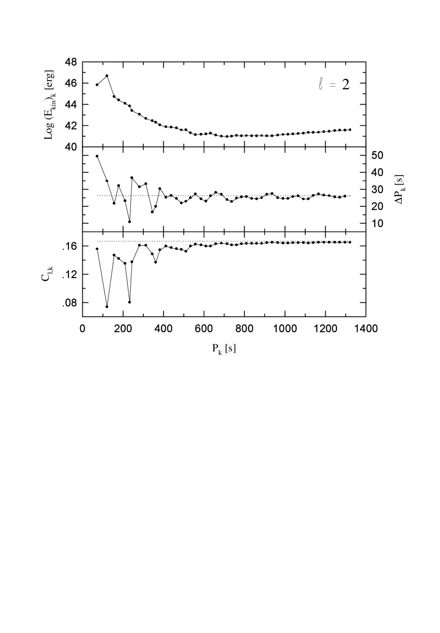
Figure 3: Same as Fig. 2, but for $\ell=2$.

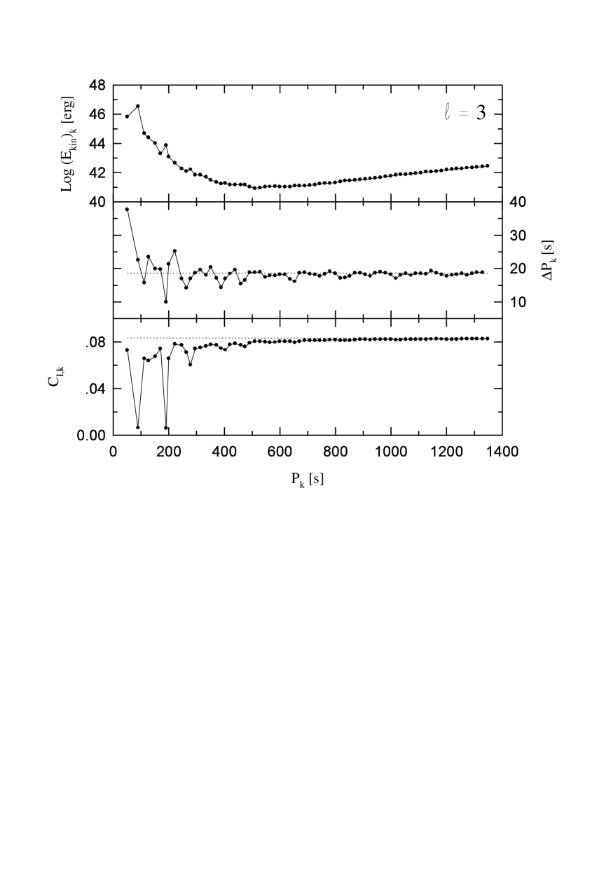
Figure 4: Same as Fig. 2, but for $\ell=3$.

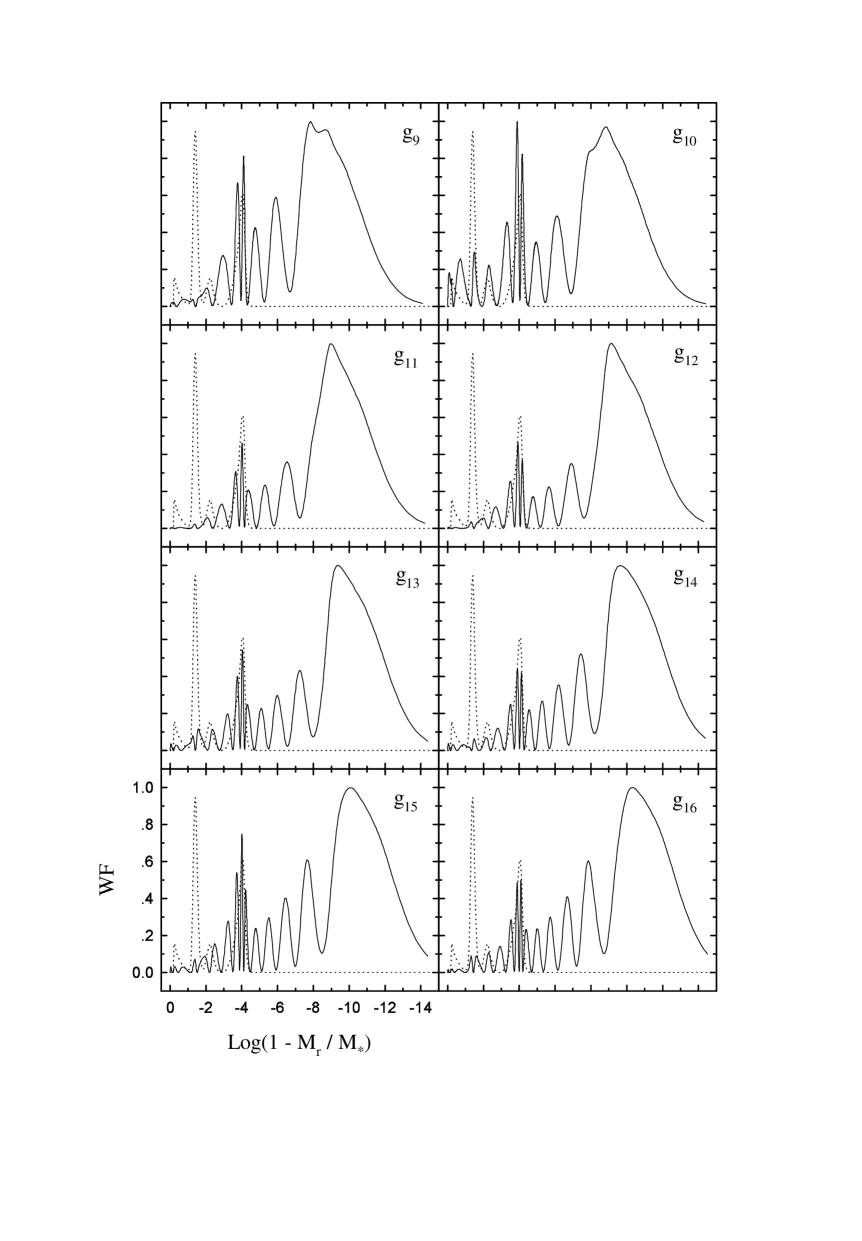
Figure 6: Same as Fig. 5, but for modes g₉ to g₁₆.

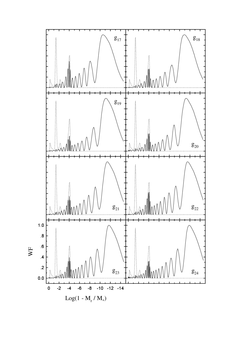
Figure 7: Same as Fig. 5, but for modes g₁₇ to g₂₄.

Figure 13: The node distribution of eigenfunctions $y_{1}$ (filled dots) and $y_{2}$ (empty dots) at the hydrogen-helium transition region for modes with $\ell=2$, according to the diffusive equilibrium prediction in the trace element approximation.

- (1) Althaus L. G., Serenelli A. M., & Benvenuto O. G., 2001, MNRAS, 323, 471
- (2) Althaus L. G., Serenelli A. M., Córsico A. H., & Benvenuto O. G., 2002, MNRAS, 330, 685
- (3) Angulo C., et al., 1999, Nucl. Phys. A, 656, 3
- (4) Böhm-Vitense E., 1958, Z. Astrophys., 46, 108
- (5) Bradley P. A., 1996, ApJ, 468, 350
- (6) Bradley P. A., 1998, ApJS, 116, 307
- (7) Brassard P., Fontaine G., Wesemael F., & Hansen C. J., 1992a, ApJS, 80, 369
- (8) Brassard P., Fontaine G., Wesemael F., & Tassoul M., 1992b, ApJS, 81, 747
- (9) Brassard P., Fontaine G., Wesemael F., Kawaler S. D., & Tassoul M., 1991, ApJ, 367, 601
- (10) Brickhill A. J., 1975, MNRAS, 170, 405
- (11) Brickhill A. J., 1991, MNRAS, 251, 673
- (12) Burgers J. M., 1969, Flow Equations for Composite Gases (New York: Academic)
- (13) Caughlan G. R., & Fowler W. A., 1988, Atomic Data and Nuclear Data Tables 40, 290
- (14) Córsico A. H., & Benvenuto O. G., 2002, Ap&SS, to be published (astro-ph: 0104267)
- (15) Córsico A. H., Benvenuto O. G., Althaus L. G., & Serenelli A. M., 2002, MNRAS, to be published (astro-ph: 0201225)
- (16) Córsico A. H., Althaus L. G., Benvenuto O. G., & Serenelli A. M., 2001, A&A, 380, L17
- (17) Dolez N., & Vauclair G., 1981, A&A, 102, 375
- (18) Dziembowski W., 1977, AcA, 27, 203
- (19) Gautschy A., & Althaus L. G., 2001, A&A to be published
- (20) Gautschy A., Ludwig H., & Freytag B., 1996, A&A, 311, 493
- (21) Goldreich P., & Wu Y., 1999, ApJ, 511, 904
- (22) Kanaan A., 1996, PhD Thesis, University of Texas
- (23) Kawaler S. D., Winget D. E., & Hansen C. J., 1985, ApJ, 295, 547
- (24) Kepler S. O., & Bradley P. A., 1995, Baltic Astron., 4, 166
- (25) Landolt A. U., 1968, ApJ, 153, 161
- (26) Saio H., Winget D. E., & Robinson E. L., 1983, ApJ, 265, 982
- (27) Tassoul M., 1980, ApJS, 43, 469
- (28) Tassoul M., Fontaine G., & Winget D. E., 1990, ApJS, 72, 335
- (29) Unno W., Osaki Y., Ando H., Saio H., & Shibahashi H., 1989, Nonradial Oscillations of Stars, University of Tokyo Press, 2nd. Edition
- (30) Winget D. E., 1988, in IAU Symp. 123, Eds. E. J. Christensen - Dalsgaard, S. Frandsen (Dordrecht Reidel), p. 305
- (31) Winget D. E., van Horn H. M., & Hansen C.J., 1981, ApJ, 245, L33
- (32) Winget D. E., Van Horn H. M., Tassoul M., Hansen C. J., Fontaine G., & Carroll B. W., 1982, ApJ, 252, L65