Mass-Loss Rate Determination for the Massive Binary V444 Cyg using 3-D Monte-Carlo Simulations of Line and Polarization Variability

A newly developed 3-D Monte Carlo model is used, in conjunction with a multi-line non-LTE radiative transfer model, to determine the mass-loss rate of the Wolf-Rayet (W-R) star in the massive binary V444~Cyg (WN5+O6). This independent estimate of mass-loss rate is attained by fitting the observed He i $5876$ Å and He ii $5412$ Å line profiles, and the continuum light curves of three Stokes parameters $\left(I,\,Q,\,U\right)$ in the $V$ band simultaneously. The high accuracy of our determination arises from the use of many observational constraints, and the sensitivity of the continuum polarization to the mass-loss rate. Our best fit model suggests that the mass-loss rate of the system is $\dot{M}_{\mathrm{WR}}=0.6\left(\pm 0.2\right)\times 10^{-5}\,M_{\sun}\,\mathrm{yr}^{-1}$, and is independent of the assumed distance to V444~Cyg. The fits did not allow a unique value for the radius of the W-R star to be derived. The range of the volume filling factor for the W-R star atmosphere is estimated to be in the range of $0.050$ (for $R_{\mathrm{WR}}=5.0\,R_{\sun}$) to $0.075$ (for $R_{\mathrm{WR}}=2.5\,R_{\sun}$). We also found that the blue-side of He i $5876$ Å and He ii $5412$ Å lines at phase $0.8$ is relatively unaffected by the emission from the wind-wind interaction zone and the absorption by the O-star atmosphere; hence, the profiles at this phase are suitable for spectral line fittings using a spherical radiative transfer model.

1 Introduction

The short-period ($P=4.212$ days, Khaliullin et al. 1984) eclipsing, massive binary V444 Cyg (WN5+O6 III-V) has been the subject of extensive studies since its discovery (e.g., Wilson 1939; Münch 1950; Shore & Brown 1988; Marchenko et al. 1994, 1997). V444 Cyg exhibits variability in polarization, line strength and X-ray flux as a function of orbital phase. The variability arises from occultation of the photosphere, from perturbations induced in the extended atmosphere of the Wolf-Rayet star (W-R) by the O star and its wind, and from the wind-wind interaction region. Despite the complexities, many authors (Hamann & Schwarz 1992; St-Louis et al. 1993; Marchenko et al. 1994; Cherepashchuk et al. 1995; Moffat & Marchenko 1996; Marchenko et al. 1997; Stevens & Howarth 1999) have used this object to determine fundamental parameters of the W-R star.

One of the most important and uncertain parameters in the stellar evolution calculation of a massive star is the mass loss rate ($\dot{M}$) during the W-R star phase. Presently there are at least 6 different methods of determining the mass-loss rate of a W-R star: 1. dynamical method using the change in the orbital period of binary (e.g., Khaliullin et al. 1984), 2. polarization variation method (St-Louis et al. 1988), 3. X-ray spectra synthesis method using a hydrodynamical model (e.g., Stevens et al. 1996; Pittard & Corcoran 2002), 4. radio/IR continuum flux method (e.g. Wright & Barlow 1975), 5. radiative transfer method (e.g., Hillier 1989; Schmutz et al. 1989) and 6. photometric variability method (e.g., Lamontagne et al. 1996). The mass-loss rate estimated from methods 4 and 5 are, in general, about $2-3$ times higher than the values estimated from methods 1, 2 and 3.

In the case of V444 Cyg, the mass-loss rate measured from the orbital period change by Khaliullin et al. (1984), Underhill et al. (1990) and Antokhin et al. (1995) are $\dot{M}_{\mathrm{WR}}=1.0\times 10^{-5}M_{\sun}\,\mathrm{yr}^{-1}$, $\dot{M}_{\mathrm{WR}}=0.4\times 10^{-5}M_{\sun}\,\mathrm{yr}^{-1}$ and $\dot{M}_{\mathrm{WR}}=0.7\times 10^{-5}M_{\sun}\,\mathrm{yr}^{-1}$ respectively. (See also Table 1.) Prinja et al. (1990) found $\dot{M}_{\mathrm{WR}}=2.4\times 10^{-5}\,M_{\sun}\mathrm{yr}^{-1}$ from the free-free radio emission flux. By modeling the infrared lines, Howarth & Schmutz (1992) obtained $\dot{M}_{\mathrm{WR}}=\left(2.5-5\right)\times 10^{-5}\,M_{\sun}\,\mathrm{yr}^{-1}$. More recently, Nugis et al. (1998) published the “clumping-corrected” mass-loss rates for 37 W-R stars from the radio emission power and the spectral index $\left(\alpha=d\ln f_{\nu}/d\ln\nu\right)$. They obtained $\dot{M}_{\mathrm{WR}}=0.92\times 10^{-5}\,M_{\sun}\,\mathrm{yr}^{-1}$ for V444 Cyg.

Hamann & Schwarz (1992), by using a non-LTE radiative transfer model with a spherically expanding atmosphere, simultaneously fitted a set of helium emission lines and the light curve of V444 Cyg. The mass-loss rate estimated from their analysis is $\dot{M}_{\mathrm{WR}}=1.26\times 10^{-5}\,M_{\sun}\,\mathrm{yr}^{-1}$. Similar to Methods 4 and 5 mentioned above, the model assumes no clumps in the stellar wind of the W-R star; hence, the mass-loss rate value is most likely overestimated. An important conclusion of their work is that the light curve is very sensitive to the inclination angle which must be treated as a fitting parameter.

St-Louis et al. (1988, hereafter STL1) derived an analytical expression for the mass-loss rate of a W-R star in a binary system, based on the model of Brown et al. (1978) which predicts the continuum polarization from a binary system as a function of orbital phase. The original model of Brown et al. (1978) assumes point sources and a single scattering atmosphere (optically thin). In the same paper, STL1 estimated $\dot{M}_{\mathrm{WR}}$ of V444 Cyg to be $0.9\times 10^{-5}\,M_{\sun}\,\mathrm{yr}^{-1}$ assuming $V_{\infty}=2500\,\mathrm{km}\,\mathrm{s}^{-1}$. Later St-Louis et al. (1993, hereafter STL2) corrected this value to $\dot{M}_{\mathrm{WR}}=0.6\times 10^{-5}\,M_{\sun}\,\mathrm{yr}^{-1}$ using the new estimate of $V_{\infty}=1785\,\mathrm{km}\,\mathrm{s}^{-1}$ (Prinja et al. 1990). STL2 also derived analytical expressions of Q & U Stokes parameters as a function of orbital phase especially near the secondary eclipse where the W-R is eclipsed by the O star. The observed polarization curves were fitted with their model, and the mass-loss rate of the W-R star in V444 Cyg was estimated ($0.75\times 10^{-5}\,M_{\sun}\,\mathrm{yr}^{-1}$). Although these models are very simple and potentially powerful, the validity is still in question since the models assume that the W-R star has a smooth wind and its atmosphere is optically thin. In addition, the derived expression of $\dot{M}_{\mathrm{WR}}$ in STL1 and $Q$ & $U$ in STL2 involves an integral which diverges. To avoid the infinity, they fixed the lower radial integration limit to $\sim 2R_{*}$.

Another important, but still uncertain parameter for V444 Cyg is the luminosity ratio, $q=L_{\mathrm{WR}}/L_{\mathrm{O}}$. Beals (1944) spectroscopically estimated $q$ for the wavelength range $4000-5000$Å. He obtained $q=0.21$ using the emission lines, and $q=0.19$ using the absorption lines. For the same system, Cherepashchuk et al. (1995) estimated the value of $q$ in a similar manner as Beals (1944), but with some modification to the calculation of the equivalent width of the emission/absorption lines. They found $q=0.60\pm 0.06$ for $\lambda\lambda$4000–6000; however, the values from different lines show a large scatter, ranging from 0.36 to 0.80. From the two principal emission lines used in these studies, they found $q=0.51$ using He ii $5412$ Å and $q=0.59$ using He i $5876$ Å (see their Table 1). Lastly, Hamann & Schwarz (1992) estimated $q=3.1$ according to their models of the light curve and helium spectrum, but the value is most likely incorrect since the effect of clumping was not included in their model.

The time dependent spectrum of the helium lines obtained by Shore & Brown (1988), Underhill et al. (1988), Marchenko et al. (1994), Marchenko et al. (1997) and Stevens & Howarth (1999) shows very complex variability associated with the orbital motion of the stars and the bow shock. Although the terminal velocities of the O star ($2540\,\mathrm{km}\,\mathrm{s}^{-1}$: Underhill et al. 1988) and the W-R star ($1785\,\mathrm{km}\,\mathrm{s}^{-1}$: Prinja et al. 1990) are comparable, the W-R star has a much denser wind, c.f., $\dot{M}_{\mathrm{O}}\approx 0.6\times 10^{-6}\,M_{\sun}\,\mathrm{yr}^{-1}$ (Leitherer 1988; Marchenko et al. 1997) and $\dot{M}_{\mathrm{WR}}\approx\left(0.4-1.26\right)\times 10^{-5}\,M_{\sun}\,\mathrm{yr}^{-1}$ (Table 1). The momentum carried by the W-R wind is several times larger than that of the O star wind, and the bow shock produced from the colliding stellar winds is folded toward the O star. Further, the orbital speed of the binary is a significant fraction of the terminal velocity of the W-R stellar wind ($V_{\mathrm{orb}}/V_{\infty}\sim 1/4$ ); hence, the shape of the bow shock is not expected to be cylindrically symmetric around the axis joining the center of the W-R star and the O star. In addition, the bow shock is not smooth, i.e., the shape of the shock front is distorted by instabilities (see Stevens & Pollock 1994; Gayley et al. 1997; Pittard 1998; Pittard & Stevens 1999) — the Kelvin-Helmholtz and the non-linear thin-shell instabilities discussed in Chandrasekhar (1961), Vishniac (1983), Vishniac (1994) and Blondin & Marks (1996).

The first X-ray evidence of the colliding winds (CWs) in V444 Cyg was found by Moffat et al. (1982) from the flux variability seen in Einstein Observatory data. In addition, Corcoran et al. (1996) and Maeda et al. (1999) found a similar X-ray variability using ROSAT and ASCA respectively. Theoretical aspects of CW related X-ray variability have been developed by, for example, Luo et al. (1990), Usov (1990), Usov (1992), Stevens et al. (1992), Myasnikov & Zhekov (1993) and Pittard & Stevens (1997).

In a previous paper (Kurosawa & Hillier 2001, hereafter, Paper I), we developed a 3-D Monte-Carlo radiative transfer model which predicts the level of continuum and line polarization produced by scattering of light in a stellar atmosphere with arbitrary geometry. The model can predict the variability features associated with orbital motion of a binary system, including the polarization level, the flux level and line profile shapes. The model can treat a finite sized stellar disk, multiple scattering, line absorption of the continuum photons and emission from multiple light sources. To achieve high precision with a minimum of data points (i.e. to save computer memory), an 8-way tree data structure created via a “cell-splitting” method (e.g, Wolf et al. 1999) is used in the model. This method is essential since the model assumes no symmetry in the atmosphere. A logarithmic grid, which is commonly used in spherical and axi-symmetric codes, is not readily implementable in a model of arbitrary geometry.

The goal of this paper is to apply the 3-D Monte-Carlo model developed in Paper I to V444 Cyg, and to interpret the observed variability features (seen in the continuum polarization and line profile shape) as a function of orbital phase. We estimate the mass-loss rate of the W-R component in the binary, the orbital inclination, and the luminosity ratio of the two stars, by fitting the observed He i $5876$ Å and He ii $5412$ Å line profiles, and the continuum light curves of three Stokes parameters $\left(\textrm{I},\,Q,\,U\right)$ in the $V$ band consistently. Unlike the radio/IR/spectral methods discussed earlier, the derived mass-loss rate determined by the polarization method is insensitive to the amount of clumps in the stellar wind. The continuum polarization level is proportional to the electron number density while the thermal emissivity (of radio/IR) is proportional to the square of the density. With a complicated density distribution, a Monte Carlo simulation provides the only method to realistically predict variability in polarization, continuum flux and line strength. An original aim was also to obtain improved estimates of the stellar parameters such as the radii of the W-R star and the O star, the monochromatic luminosity ratio of the two stars and the orbital inclination angle. Due to both model and observation uncertainties, this proved not to be feasible.

In § 2, we discuss our models, examine the variability of He i $5876$ Å and He ii $5412$ Å lines, and determine the mass-loss rate of the Wolf-Rayet star in V444 Cyg. The discussion on the results will be given in § 3, and the conclusion in § 4.

Table 1: Basic Parameters of V444 Cyg.

	PUBLISHED VALUES
$\dot{M}_{\mathrm{WR}}$  $\left[\times 10^{-5}\,M_{\odot}\,\mathrm{yr}^{-1}\right]$	$0.6^{\left(a\right)}$, $1.0^{\left(b\right)}$, $0.4^{\left(c\right)}$, $\left(0.8_{-0.3}^{+0.5}\right)^{\left(d\right)}$, $0.7^{\left(v\right)}$, $0.9^{\left(w\right)}$
	$2.4^{\left(e\right)}$, $2.5-5.0^{\left(f\right)}$, $1.26^{\left(g\right)}$, $0.92^{\left(o\right)}$
$q\,\left[=L_{\mathrm{WR}}\left(\lambda\right)/L_{\mathrm{O}}\left(\lambda\right)\right]$	$0.6\pm 0.06^{(h)}$ for $\lambda\lambda 4000-6000$ Å
	$\sim 0.2^{\left(i\right)}$ $\lambda\lambda 4057-6563$ Å
	$0.25-0.35^{\left(j\right)}$ for $\lambda\lambda 4400-10000$ Å
$R_{\mathrm{WR}}\,\left[R_{\sun}\right]$	$2.9^{\left(r\right)}$, $<4^{\left(a\right)}$, $6.31^{\left(g\right)}$, $3.1-5.2^{\left(s\right)}$
$R_{\mathrm{O}}\,\left[R_{\sun}\right]$	$8.5\pm 1^{\left(a\right)}$, $10.0^{\left(r\right)}$, $3.76^{\left(g\right)}$, $8.4-9.3^{\left(s\right)}$
$i\,\left[\mathrm{deg}.\right]$	$82.8\pm 0.9^{\left(l\right)}$, $78.8\pm 0.5^{\left(m\right)}$, $80.8\pm 1.6^{\left(a\right)}$, $83.47^{\left(g\right)}$
$M_{v}^{\left(*\right)}$ (O+W-R)	$-5.7^{\left(n\right)}$ , $-4.2^{\left(g\right)}$
$m_{v}$ (O+W-R)	$8.27^{\left(n\right)}$
$DM$	$11.01\pm 0.20^{\left(u\right)}$, $11.27-11.47^{\left(d\right)}$, $9.3^{\left(g\right)}$
Mass (O:W-R) $\left[M_{\sun}\right]$	$25$ : $10^{\left(p\right)}$, $27.9$$\left(\pm 3.2\right)$ : $9.3\left(\pm 1.0\right)^{\left(q\right)}$, $37.5$ : $11.3^{\left(t\right)}$

($a$) St-Louis et al. (1993), ($b$) Khaliullin et al. (1984), ($c$) Underhill et al. (1990), ($d$) Marchenko et al. (1997), ($e$) Prinja et al. (1990), ($f$) Howarth & Schmutz (1992), ($g$) Hamann & Schwarz (1992), ($h$) Cherepashchuk et al. (1995), ($i$) Beals (1944), ($j$) Kuhi (1968), ($k$) Cherepashchuk (1975), ($l$) Piirola & Linnaluoto (1988), ($m$) Robert et al. (1990), ($n$) Lundström & Stenholm (1984), ($o$) Nugis et al. (1998), ($p$) Münch (1950), ($q$) Marchenko et al. (1994), ($r$) Cherepashchuk et al. (1984), ($s$) Moffat & Marchenko (1996), ($t$) Underhill et al. (1988), ($u$) Forbes et al. (1992), ($v$) Antokhin et al. (1995), ($w$) Rodrigues & Magalhaes (1995).

$\left(*\right)$ assumed the distance to be 1.7 kpc and $E_{b-v}=0.68$ Lundström & Stenholm (1984) – They assumed the intrinsic color to be $\left(b-v\right)_{\mathrm{o}}=-0.30$.

2 Analysis

The five most important parameters which we initially hoped to constrain in our analysis were: the mass-loss rate of the W-R star ($\dot{M}_{\mathrm{WR}}$), the luminosity of the W-R star ($L_{\mathrm{WR}}$), the radius of the W-R star ($R_{\mathrm{WR}}$), the volume filling factor ($f$) and the monochromatic luminosity ratio of the W-R and O stars, $q\left(\lambda\right)=L_{\mathrm{WR}}\left(\lambda\right)/L_{\mathrm{O}}\left(\lambda\right)$, at $\lambda=5630$Å. The volume filling factor is defined as the fractional volume which contains material (the higher density regions or clumps), and it controls the amount of clumps in the atmosphere (see e.g., Abbott et al. 1981). It can also be thought of as the fractional length along any random line of sight which contains clumps.

Since the procedure of the model fitting is rather complicated, we summarize the steps for determining the parameters below:

1. Understand the basic behavior of the variability seen in He i $5876$ Å  and He ii $5412$ Å  lines to determine at which binary phase the spectrum is least affected by the bow shock and by the presence of the O star atmospheric absorption. In other words, determine at which phase the spectrum is modeled best by a spherical radiative transfer model (CMFGEN).

2. At the phase chosen to be the best in Step 1, fit the observed helium spectrum for different W-R star radii, and find the corresponding value of $q$. In general, $L_{\mathrm{WR}}=2\times 10^{5}\,L_{\sun}$ is used.

3. Fit the continuum I, Q, U light curves around the secondary eclipse ($\phi\approx 0.5$) to constrain the radius of the W-R star. ($q$ and $R_{\mathrm{WR}}$ are constrained.)

4. With $R_{\mathrm{WR}}$ and $q$ values determined in Step 3, re-fit the helium spectrum with different values of $\dot{M}$.

5. Compute the continuum $I$, $Q$, $U$ light curves for the $R_{\mathrm{WR}}$ , $q$ and $\dot{M}_{\mathrm{WR}}$ values used in Step 4, and fit only the $I$ light curve by adjusting the orbital inclination ($i$) and $R_{\mathrm{O}}$.

6. Now there are several models which fit the observed $I$ light curve and the helium spectrum simultaneously, but only a certain value of $\dot{M}_{\mathrm{WR}}$ will fit the $Q$ and $U$ light curves; therefore, the value of $\dot{M}_{\mathrm{WR}}$ is constrained. ($i$, $R_{\mathrm{O}}$ and $\dot{M}_{\mathrm{WR}}$ are constrained.)

2.1 Line Variability and Geometric Configuration of the Binary

Since the 3-D Monte Carlo polarization model introduced in Paper I is not a self-consistent model (i.e., the radiation does not modify the opacity of the atmosphere), the opacity and the emissivity must be supplied as the inputs of a model. There are three possible sources of the input field: 1. parametrized functions from a semi-analytical model, 2. output from a spherical non-LTE radiative transfer model with some modifications, and 3. output from a hydrodynamical calculation in conjunction with method 2. Method 1 is useful for testing models, but not suited for modeling a real object. In our analysis, method 2 is mainly used.

The first step, in method 2, is to compute the object’s spectrum using a non-LTE radiative transfer code (CMFGEN) which includes thousands of lines to treat the line-blanketing effect (Hillier & Miller 1998). For example, see Hillier & Miller (1999) and Herald et al. (2001) for a detailed discussion of W-R star spectrum models across a wide wavelength range. CMFGEN provides the opacity and the emissivity of the W-R star and the O star separately, and is designed for a single star with a “spherically” expanding atmosphere; hence, the output fields (opacities etc.) are functions of radius only. The second step is to compute the variability of the Stokes parameters ($I$, $Q$, $U$) and the line profiles by using the 3-D Monte Carlo model as a function of the binary phase.

The velocity field in a CMFGEN model is assumed to have the following form (Hillier & Miller 1999):

$$v\left(r\right)=\frac{V_{0}+V_{1}+V_{2}}{1+\left(V_{0}/V_{\mathrm{core}}-1\right)\,\exp\left[-\left(r-R_{*}\right)/h_{\mathrm{eff}}\right]}$$ (1)

where $V_{1}=\left(V_{\infty}-V_{\mathrm{ext}}-V_{0}\right)\left(1-R_{*}/r\right)^{\beta_{1}}$, $V_{2}=V_{\mathrm{ext}}\left(1-R_{*}/r\right)^{\beta_{2}}$, $h_{\mathrm{eff}}$ is an isothermal effective scale height in the inner atmosphere, $V_{\infty}$ is the terminal velocity, $V_{\mathrm{core}}$ is the expansion velocity of the core, and $V_{\mathrm{ext}}$ & $\beta_{2}$ are the parameters for the outer parts of the wind. $\beta_{1}$ is equivalent to the $\beta$ in the classic beta-velocity law, $V\left(r\right)=V_{\infty}\left(1-R_{*}/r\right)^{\beta}$, for the “inner part” of the stellar wind. See Najarro et al. (1997) and Hillier & Miller (1999) for more explanations on this velocity law. Although the line-driving of O-star winds is well understood, the multiple-scattering of W-R winds complicates theoretical models, and the standard CAK theory (Castor, Abbott, & Klein 1975) does not apply for W-R stars.

Fig. 1 shows the basic configuration of the model geometry. The W-R star with its extended atmosphere is located at the center. Surrounding the O star, the bow shock due to the CWs has a paraboloidal shape, and points away from the W-R star since its wind is much stronger than that of the O star. The head of the shock front is tilted from the purely radial direction because of the rapid orbital motion. Using the ratio of the terminal velocity of the W-R component ($V_{\infty}=1785\,\mathrm{km}\,\mathrm{s}^{-1}$, Prinja et al. 1990) and the orbital speed ($V_{\mathrm{orb}}\approx 460\,\mathrm{km}\,\mathrm{s}^{-1}$), the tilt angle of the bow shock region can be estimated as $\delta\simeq\tan^{-1}(V_{\mathrm{orb}}/V_{\infty})\approx 15^{\circ}$. Extensive discussions on the morphology of the bow shock can be found in Marchenko et al. (1997), including the issue of whether the W-R wind is impacting onto the O star surface or not. (See also the hydrodynamical calculation of Pittard & Stevens 1999).

At $\phi$ (orbital phase) $=0$, the W-R star is in front of the O star, and an observer is looking at the system from the top of Fig. 1 since the inclination angle $i$ is about $80^{\circ}$ (almost edge-on view). At $\phi=0.5$, the O star is in front of the W-R star. The directions of an observer at $\phi=0,\,0.25,\,0.5,\,0.75$ are indicated in the same figure, and they infer the sense of the orbital motion (counter-clockwise in the figure). The strong stellar wind from the W-R star is interrupted by the shock front, and the density behind the shock is assumed to be negligibly small for simplicity. In other words, we do not include the O star wind explicitly, and we place the bow shock zone rather artificially.

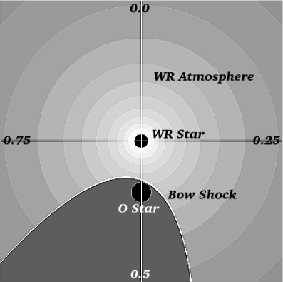
Figure 1: This figure illustrates the model configurations of V444 Cyg. The W-R star is placed at the center of the cubic boundary, and it is surrounded by a spherical atmosphere which is consistent with the CMFGEN spectral model. The O star is located below the W-R star in the diagram, and is covered by the tilted paraboloid bow shock with a given thickness. The strong stellar wind from the W-R star is interrupted by the shock front, and the density behind the shock is assumed to be negligibly small for simplicity. The directions of an observer at phase $=0,\,0.25,\,0.5,\,0.75$ are indicated at the top, bottom, left and right edges since the orbital inclination is about $80^{\circ}$ (almost edge-on view).

Next, we propose a simple model of the gas flow in the CW zone and the geometry of the CW zone. We assume the shape of the CW zone to be paraboloid with thickness $d$. The center of the paraboloid is located along the y-axis but displaced by $y_{o}$ from the origin as shown in Fig. 2. The surface of the paraboloid can be written as:

$$y=a_{y}l^{2}+y_{o}$$ (2)

where $l^{2}=x^{2}+z^{2}$. We define the bow shock region to be the volume between this surface and the same surface displaced by $d$ (thickness) in $+y$ direction.

The flow of the gas in the CW zone is assumed to be tangential to the surface of the paraboloid; hence, there is no azimuthal component. Then, the velocity ($\mathbf{v}_{\mathrm{cw}}$) of the gas flow at point $P$ in the CW zone can be written as:

$$\mathbf{v}_{\mathrm{cw}}=v_{y}\hat{\mathbf{y}}+v_{l}\hat{\mathbf{l}}$$ (3)

where $\hat{\mathbf{l}}=\cos\phi_{c}\hat{\mathbf{z}}+\sin\phi_{c}\hat{\mathbf{x}}$. $v_{y}$ and $v_{l}$ are the velocity components which are parallel and perpendicular to the y axis, respectively. $a_{y}$ is a parameter to control the asymptotic open angle of the bow shock. Further, by taking the derivative of Eq. 2 and using the absence of an azimuthal component of $\mathbf{v}_{\mathrm{cw}}$, we obtain:

$$\frac{dy}{dl}=2a_{y}l=\frac{v_{y}}{v_{l}}\,.$$ (4)

If the magnitude of the velocity ($\mathbf{v}_{\mathrm{cw}}$) at point $P$ is similar to that of the spherical flow ($v_{r}$) of the pre-shock W-R wind at $P$ , i.e., $v_{\mathrm{cw}}\approx v_{r}$, then

$$v^{2}_{r}\approx v^{2}_{y}+v^{2}_{l}\,.$$ (5)

Since the flow of gas in the bow shock region is usually slower than the surrounding flow according to the hydrodynamics model of Pittard & Stevens (1999), we introduce a free parameter, and rewrite the equation above as:

$$v_{\mathrm{cw}}=s\,v_{r}=\left(v_{y}^{2}+v^{2}_{l}\right)^{1/2}.$$ (6)

In general $s<1$, and is a function of the position (e.g., $s=s\left(y\right)$). However, in most of the analysis, $s=1/2$ is assumed for simplicity.

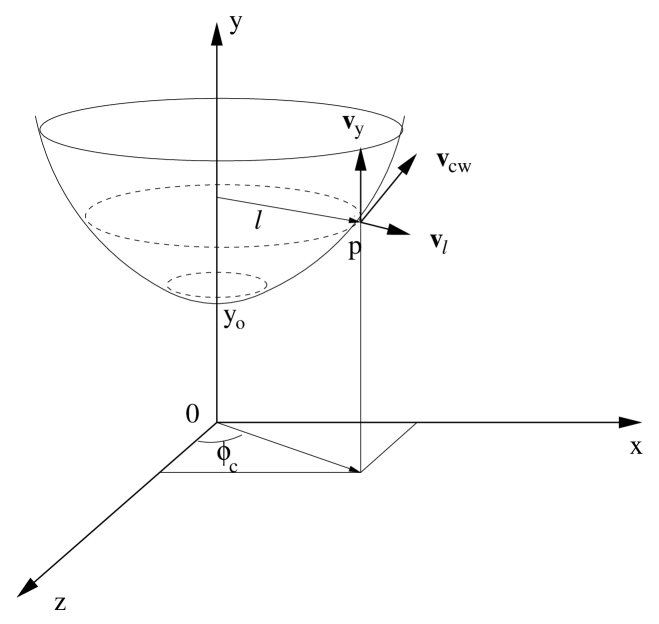
Figure 2: This illustrates the simple geometric model of the bow shock and the flow of the gas. The W-R star is located at the origin (0), and the O star is located just behind the bow shock on the y axis. The gas in the bow shock region is assumed to flow tangentially to the surface of the paraboloid in the $+y$ direction. The gas velocity $\mathbf{v}_{\mathrm{cw}}$ at a point $p$ on the surface is decomposed into $v_{y}$ and $v_{l}$, but there is no azimuthal component (i.e., no rotation about the $y$ axis).

Using Eqs. 4, 5 and 6, the components of $\mathbf{v}_{\mathrm{cw}}$ can be expressed, in terms of the position $\left(y,\,l\right)$ on the paraboloid, as

$$v_{y}=\frac{2a_{y}\,l\,s\,v_{r}}{\left[1+\left(2a_{y}l\right)^{2}\right]^{1/2}}\,,$$ (7)

and

$$v_{l}=\frac{s\,v_{r}}{\left[1+\left(2a_{y}\,l\right)^{2}\right]^{1/2}}\,.$$ (8)

These expressions are then corrected for the tilt of the bow shock due to the fast orbital motion of the system, as mentioned earlier. A more accurate velocity field in the bow shock region is needed to properly model the line profile and the line polarization, but it is not important for the continuum calculations.

Considering the radial dependence of the density, we define:

$$\rho_{\mathrm{shock}}=\rho_{\mathrm{o}}\left(\frac{y_{\mathrm{o}}}{r}\right)^{n}$$ (9)

where $r$ is the distance between the origin ($0$) and a point $p$ on the surface of the parabola, and $y_{\mathrm{o}}$ is the distance between the origin and the head of the paraboloid as shown in Fig. 2. The index $n$ is a scaling parameter, and $\rho_{\mathrm{o}}$ is the density at the head of the parabola (at $y=y_{\mathrm{o}}$). This formulation is similar to one in Stevens & Howarth (1999). $\rho_{\mathrm{o}}$ is estimated from the amount of the excess emission seen in the He i $5876$ Å line, and is discussed in the later section (§ 2.2.3). In our analysis, we use the bow shock density expressed in Eq. 9 with $n=2$, and the thickness ($d$) of the bow shock $\approx 0.1\,R_{\mathrm{O}}$, estimated from Pittard & Stevens (1999). In predicting the continuum polarization level, the global distribution of the electron density is more important than small structure. The column density or the electron scattering opacity through the bow shock is related to the amount of gas in the cavity which will be absent if there is no bow shock.

Some sensitivity of the line strengths and polarization may arise from assuming whether the helium is singly or doubly ionized. He i $5876$ Å and He ii $5412$ Å lines are often referred to as “diagnostic lines” for modeling a WN star atmosphere (e.g., Hamann et al. 1995). The latter is an optically thick line; hence, the absorption and scattering terms in radiative transfer equations must be treated properly. The gas in the bow shock is rapidly cooled by radiative processes, and it could potentially cause a significant amount of absorption in the He i $5876$ Å line. Figure. 3 shows the approximate location where He i $5876$ Å and He ii $5412$ Å lines originate according to a CMFGEN model of a typical WN5 star with $R_{\mathrm{WR}}=5\,R_{\sun}$. The figure shows that the He ii emission peaks at around $3\,R_{\mathrm{WR}}$ from the center of the W-R star, and the He i emission peaks around the location where the O star resides. This explains why the emission from the CW zone is more clearly seen in the He i line. In the following, the variability of the He i line due to the presence of the bow shock will be examined.

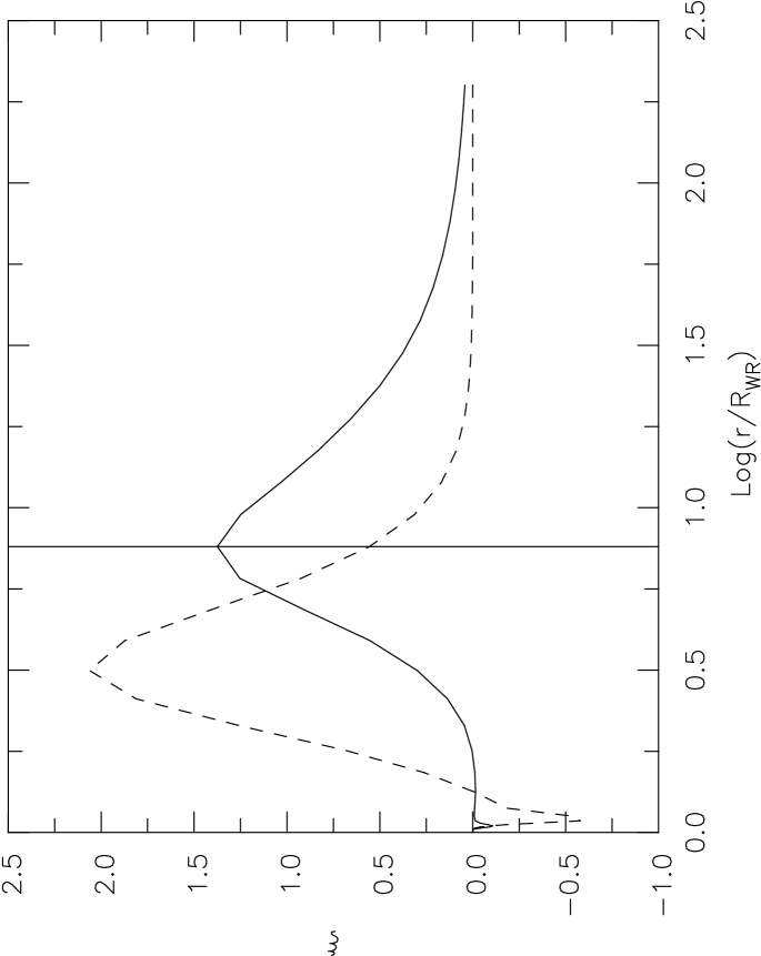
Figure 3: Illustration of the approximate location where He i $5876$ Å (solid) and He ii $5412$ Å  (dashed) lines originate according to a CMFGEN model of a typical WN5 star with $R_{\mathrm{WR}}=5\,R_{\sun}$. The amount of line emission originating in the interval $d\log\left(r/R_{\mathrm{WR}}\right)$ is proportional to $\xi\,d\log\left(r/R_{\mathrm{WR}}\right)$ where $r$ is the distance from the center of the W-R star. The solid vertical line at $\log\left(r/R_{\mathrm{WR}}\right)=0.88$ indicates the location of the O star assuming that the separation of system is $a=38\,R_{\sun}$ (Marchenko et al. 1994). According to this figure, the He ii  emission peaks at around $3\,R_{\mathrm{WR}}$ from the center of the W-R star, and the He i  emission peaks around the location where the O star resides.

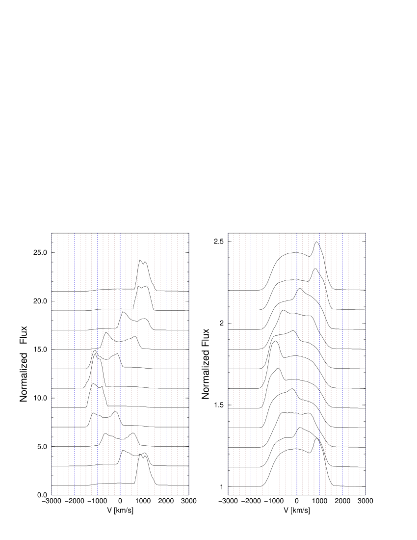
Figure 4: Left: The phase dependent emission from the bow shock region on top of He i $5876$ Å line. The emissivity of the bow shock is assigned to be unrealistically strong in order to demonstrate its effect more clearly. Right: As for the left figure, but the emissivity of the bow shock is reduced by a factor of $\sim 10$. This figure qualitatively describes the variability seen in the observation of this line (e.g., see Marchenko et al. 1994). The profiles are plotted from phase $=0$ (bottom) to phase $=1$ (top) in 0.1 phase steps. The profiles are normalized to continuum, and shifted upward by 2 (right) and 0.12 (left) consecutively at each phase. In these models, the tilt angle $\delta=15^{\circ}$ and $\mathrm{open}\,\mathrm{angle}=90^{\circ}$ (Marchenko et al. 1994) are used.

2.1.1 Effect of the Colliding Winds

As explained earlier, the emission from the bow shock region is prominent for some lines (see Marchenko et al. 1994). In this section, the expected effect of the bow shock emission on the He i $5876$ Å line will be demonstrated using the 3-D Monte Carlo model. He i $5876$ Å is primarily a recombination line; hence, to first order we assume the line emissivity in the bow shock region is simply proportional to the square of the density. The tilt angle $\delta=15^{\circ}$ and the $\mathrm{open}\,\mathrm{angle}=90^{\circ}$ (Marchenko et al. 1994) are used for the geometry of the bow shock. The left graph in Fig. 4 shows a sequence of He i $5876$ Å emission lines as a function of phase ($0-1$ with steps of $0.1$ from the bottom) arising from a V444 Cyg model which includes an unrealistically strong bow shock emission. In fact, the line emission is dominated by the bow shock emission, and the underlying line emission from the W-R atmosphere is barely visible in this figure. This plot demonstrates the basic behavior of the emission from the bow shock region. (See also Lührs 1997 and Bartzakos et al. 2001 for similar models and discussion.) At $\phi=0.8-1.0$, the bow shock is pointing away from an observer and tilted to the light of sight (Fig. 1); therefore, the emission peak appears on the red side of the flat-top He i emission line. The shape of the CW emission changes very rapidly from $\phi=0$ to $0.1$ because a rapid change in the velocity component of the bow shock arms along the line of sight occurs near $\phi=0.1$. The emission from the bow shock flattens out during $\phi=0.1-0.4$ and $\phi=0.7-0.8$ since the bow shock arms are almost perpendicular to the direction of the observer. At $\phi=0.4-0.5$, the peak appears on the blue side since the bow shock arms are pointing towards an observer. A sequence of He i $5876$ Å line profiles with a more realistic level of bow shock emission is shown in the right panel of Fig. 4. The figure shows that the line strength increases around $\phi=0$ and $0.5$ because the continuum level drops during the primary and secondary eclipses.

2.1.2 O star Absorption Effect

The observed spectrum of V444 Cyg shows absorption lines due to the O star atmosphere on top of the broad emission lines from the W-R atmosphere. The position of absorption shifts as the relative speed of the stars changes. The distortion caused by this effect is prominent for some lines at certain binary phases. Since the model does not take into account the photospheric spectrum of the O star, the O star absorption lines have been added to the CMFGEN model in an approximate manner. In principal they could easily be incorporated into the Monte Carlo method by changing the appropriate boundary conditions.

The O star component of V444 Cyg has spectral type O5-O6.5 III-V (Marchenko et al. 1994). The O star (O6) spectrum is modeled separately by CMFGEN, and the effect of the rotational broadening of lines is added to the spectrum. In this process, the rotational speed $V_{\mathrm{rot}}\,\sin i=215\,(\pm 13)\,\mathrm{km}\,\mathrm{s}^{-1}$ (Marchenko et al. 1994) is used.

Fig. 5 shows the combined spectrum of the W-R and the O star computed by CMFGEN as a function of the orbital phase. The sinusoidal motion of the O star absorption component is clearly seen in both lines. To examine only the effect of the O star, the emission from the CW zone is not included in the model spectra shown in this figure. A specific luminosity ratio ($q=L_{\mathrm{WR}}/L_{\mathrm{O}}=0.45$ at $\lambda=5630$ Å) was used when the two spectra were combined.

Figure 5: The figure illustrates how the O star absorption affects the appearance of the He i $5876$ Å and He ii $5412$ Å lines from the W-R atmosphere as a function of the orbital phase ($\phi$). The spectrum of the W-R and the O stars computed with the spherical model, CMFGEN, are combined using the monochromatic luminosity ratio, $q=L_{\mathrm{WR}}/L_{\mathrm{O}}=0.45$ at $\lambda=5630$ Å. The figure does not include the effect of the colliding wind for clarity. The profiles are plotted from $\phi=0$ (bottom) to $\phi=1$ (top) with 0.1 phase steps.

2.1.3 Combined Effects Compared with Observation

In order to use CMFGEN for the model fitting, we must choose a binary phase when the lines are least affected by the bow shock emission and the O star absorption. Fig. 5 shows that the absorption by the O star does not affect the overall shape of He i $5876$ Å, but it does affect the shape of He ii $5412$ Å. At $\phi\approx 0.2$ and $\phi\approx 0.7$, the He i line shape is least affected by the O star, but at these phases the emission from the bow shock region is spread over the He i line as seen in Fig. 4. As a result, the line flux level is likely slightly higher than that of the spherical model. On the other hand, at $\phi\approx 0$ and $\phi\approx 0.5$, the emission from the bow shock region is well concentrated near the blue or the red edge of the He i line, but at these phases, the stars are eclipsed; hence, the line strength will be underestimated in a simple spherical model (CMFGEN). Meanwhile at $\phi\approx 0.3$ and $\phi\approx 0.8$, the bow shock emission is concentrated only on either the blue or the red side of the He i line, and the O star absorption affects the same half side of the line profile. Unfortunately, at $\phi\approx 0.3$, the O star absorption is on the red side of the helium line, and the bow shock emission is on the blue side of the line. So the line is contaminated on both sides. On the other hand at $\phi\approx 0.8$, both the O star absorption and the emission from CW are on the red side of a line; hence we can reliably use the blue part of He i $5876$ Å and He ii $5412$ Å for the model fitting. Figure 6 shows the sample CMFGEN model spectrum compared with the observed spectrum of Marchenko at six different phases. The agreement between the model and the observation at $\phi\approx 0.8$ is excellent. Near the eclipsing phases ($\phi\approx 0$ and $0.5$), the spherical model CMFGEN does not fit the observation well since the contribution from the bow shock is not included in the model. The two narrow Na i interstellar absorption lines are present in the red side of observed He i $5876$ Å lines.

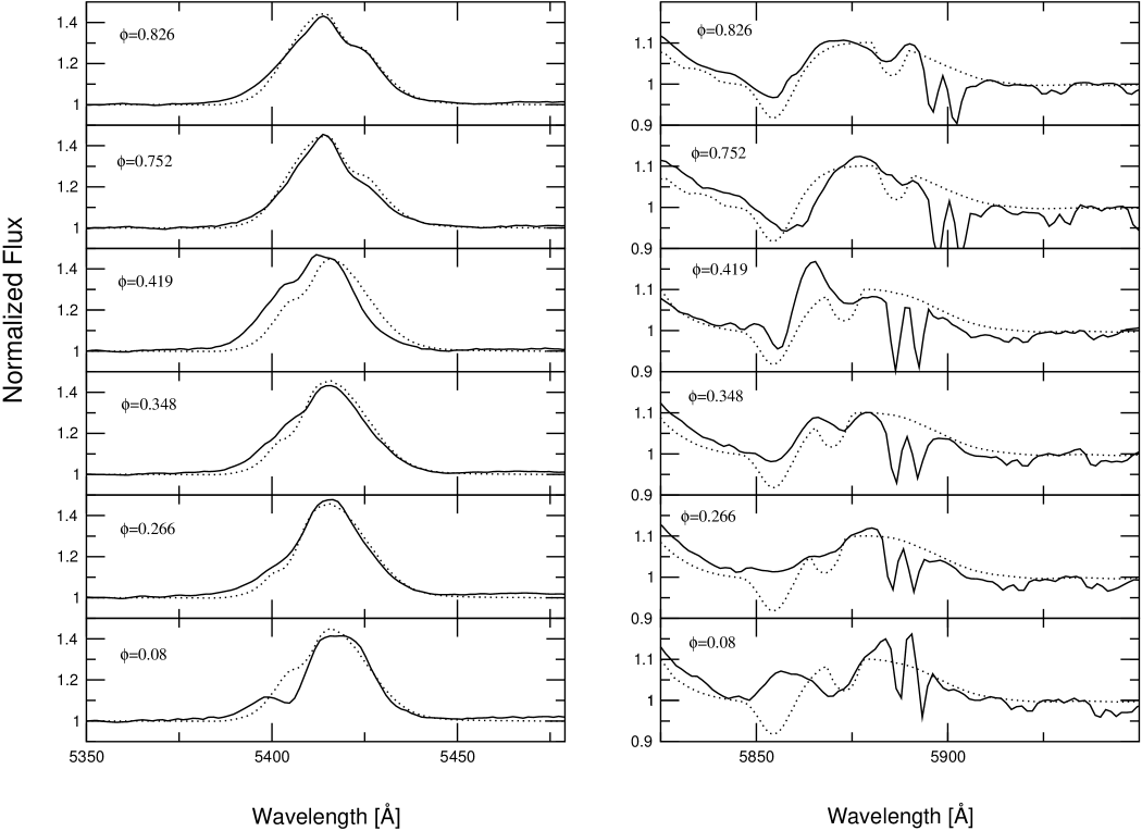
Figure 6: The figure shows one of the best fit CMFGEN models (Dotted) at 6 different binary phases. The observational data (Solid) were provided by Marchenko . The O star model spectrum (O6V) is added to include the effect of the atmospheric absorption effect. The monochromatic luminosity ratio $q=L_{\mathrm{WR}}/L_{\mathrm{O}}=0.45$ at $\lambda=5630$ Å  is used when the W-R star model spectrum is combined with the O star model spectrum. In general, the fits are good at all phases shown, especially at $\phi\approx 0.3$ and $\phi\approx 0.8$. Two narrow Na i interstellar absorption lines are present in the red side of observed He i $5876$ Å lines. The emission from the bow shock is not included in the model shown here.

2.2 Mass-Loss Rate Estimation of the W-R Component

The idea behind the mass-loss estimation performed here is very similar to the one in STL1 and STL2. We assume that there is a correspondence between the amount of continuum polarization and the mass-loss rate of the W-R component. This is supported by the analytic expression of $\dot{M}$ in terms of $A_{p}$ (a semi-major axis of polarization on Q-U plane) derived by STL1, using the basic results from the classic paper on binary polarization by Brown et al. (1978).

2.2.1 Investigation of the W-R Radius

For an assumed mass-loss rate, $\dot{M}$, of the W-R star, there are several CMFGEN models which can fit the observational spectrum of He ii $5412$ Å and He i $5876$ Å simultaneously. As discussed in the previous section, the spectrum at $\phi\approx 0.8$ is used in the model fitting since the contamination from the O star atmospheric absorption and the CW emission is expected to be small at this orbital phase. Fig. 7 shows the fits of the observed spectrum at $\phi=0.826$ for different values of $R_{\mathrm{WR}}$ (=$2.5$, $4.0$, $5.0\,R_{\sun}$) with the mass-loss rate of the W-R star fixed ($\dot{M}_{\mathrm{WR}}=0.6\times 10^{-5}\,M_{\sun}\,\mathrm{yr}^{-1}$). The corresponding volume filling factors of the models are $0.08$, $0.04$, $0.05$. All three models fit the observation very well; therefore, the spectral solutions are degenerate. The He ii profiles with different values of $R_{WR}$ are not significantly different from each other when the O star spectrum is added to the W-R spectrum with an appropriate value of $q$ ($=0.30,\,0.35,\,0.45$ for $R_{\mathrm{WR}}=2.5,\,4.0,\,5.0\,R_{\sun}$ models respectively). In the case of a single W-R star spectrum, a small but noticeable difference in the profile shape of the He ii line, usually becoming more triangular for a larger $R_{\mathrm{WR}}$, should be present. Unfortunately, it is hard to see this effect in the V444 Cyg model because the continuum flux of the O star component is stronger ($q\approx 0.5$); hence, the line strength is weakened.

In an attempt to remove this degeneracy, the light curves ($I$, $Q$, $U$) are computed by the 3-D Monte-Carlo model (Kurosawa & Hillier 2001) for the spectral models shown in Fig. 7 for fixed $R_{\mathrm{O}}$ and $\dot{M}_{\mathrm{WR}}$ values. First, models without the bow shock (Figs. 8 – 12) are considered for clarity. The effect of the bow shock on the light curve will be examined later. A small difference is expected to be seen (c.f., STL2) in the shape of the polarization curve near the secondary eclipse ($\phi\approx 0.5$, i.e., when the W-R star is behind the O star).

Figure 7: Left: the model fits of He ii $5412$ Å for three different radii ($2.5$, $4.0$ and $5.0\,R_{\sun}$) of the W-R star. Right: same as the left, but for He i $5876$ Å. The profile shapes of both lines fit the observation well for a relatively wide range of the W-R star radius. When the O star spectrum is added to the W-R spectrum with an appropriate value of $q$, the profiles with different values of $R_{\mathrm{WR}}$ are not significantly different from each other. The values of $q$ used are 0.30, 0.35 and 0.45 for $R_{\mathrm{WR}}=$2.5, 4.0 and $5.0\,R_{\sun}$ models respectively. The corresponding volume filling factors of the models are 0.08, 0.04, 0.05.

The results, using $R_{\mathrm{O}}=7.2\,R_{\sun}$ and $\dot{M}_{\mathrm{WR}}=0.6\times 10^{-5}\,M_{\sun}\,\mathrm{yr}^{-1}$, are shown in Fig. 8. The orbital inclination angles used for the fits are $i=78.8^{\circ}$, $78.5^{\circ}$ and $78.0^{\circ}$ for the models with $R_{\mathrm{WR}}=2.5\,R_{\sun}$, $4.0\,R_{\sun}$ and $5.5\,R_{\sun}$ respectively. The inclination angles are consistent with $i=78^{\circ}\pm 1^{\circ}$ (Cherepashchuk 1975) obtained from the light curve solution. STL2 estimated the inclination angle by fitting the double sine curves of $Q$ and $U$ polarization components with the formula given by Brown et al. (1978). Their result is $i=80.8^{\circ}\pm 1.6^{\circ}$. In Fig. 8, the three models fit the observed $I$ light curve moderately well. Although not shown here, all three models also fit well the observed $I$ light curve outside of the phase range shown in Fig. 8. The deviations from perfect anti-symmetry around $\phi=0.5$ seen in the observational $I$ light curve and the anomaly seen around $\phi\approx 0.53-0.54$ in the U observational light curve are not well fitted, and may be related to the presence of the bow shock in the system.

The width of the $I$ light curve around $\phi=0.5$ is slightly wider for the model with the larger W-R star radius. The $R_{\mathrm{WR}}=5.0\,R_{\sun}$ model fits the overall shape of the light curve better than the two other models with smaller radii. However, the width of the secondary eclipse depends also on the mass-loss rate of the W-R star, and we discuss this dependency later. Unfortunately, no significant difference in the Q and U light curves are seen for different values of W-R star radii, unlike that found by STL2. In fact, the difference in Q and U light curves seen by STL2 for different $R_{\mathrm{WR}}$ (see their Fig. 8) is not purely due to changing $R_{\mathrm{WR}}$, being also coupled with $\dot{M}_{\mathrm{WR}}$ and the adopted inclination.

In this analysis, we were not able to constrain the value of $R_{\mathrm{WR}}$. Models with a wide range of $R_{\mathrm{WR}}=2.5-5.0\,R_{\sun}$ can fit the observed $I$, $Q$ and $U$ light curves reasonably well, and there is no significant difference among them as long as appropriate values of the orbital inclination angle and the O star radius are chosen for each model. Despite this uncertainty in the W-R star radius, we continue to derive the mass-loss rate of the W-R star.

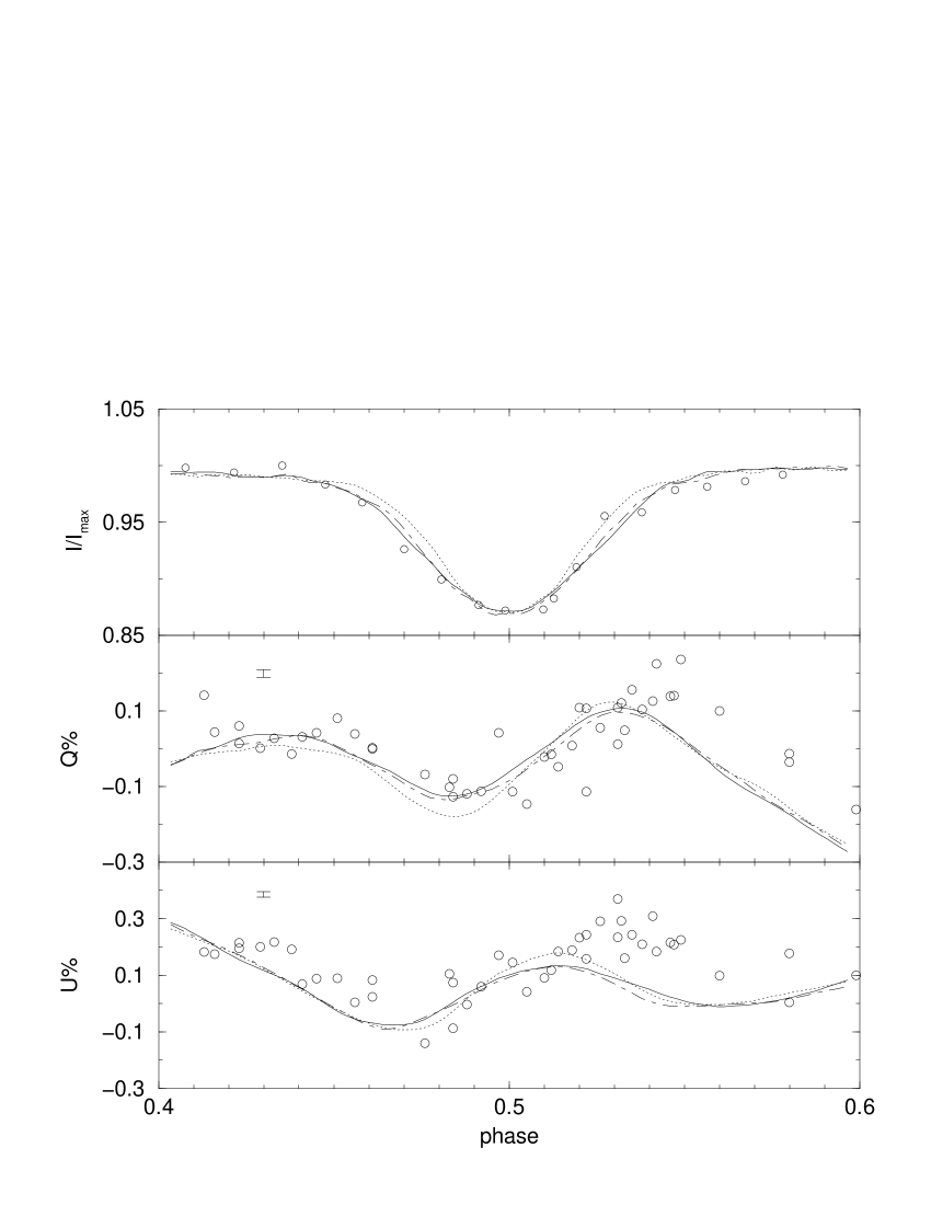
Figure 8: The continuum flux, Q and U polarization near the secondary eclipse (where the O star is in front of the W-R star) are computed by the 3-D Monte-Carlo model of Kurosawa & Hillier (2001) for the three spectral models shown in Fig. 7. Circles: Observation, Dot: $R_{\mathrm{WR}}=2.5\,R_{\sun}$ & $q=0.30$ model, Dash-Dot: $R_{\mathrm{WR}}=4.0\,R_{\sun}$ & $q=0.35$ model, Solid: $R_{\mathrm{WR}}=5.0\,R_{\sun}$ & $q=0.45$ model. The typical size of the error in model calculations of $Q$ and $U$ is indicated near the upper left corner of the middle and the bottom plots. The optical light curve data and optical polarization data (V band) are from Kron & Gordon (1943) and STL2 respectively.

2.2.2 Determination of the W-R Mass-Loss Rate

Next, the observed helium spectrum is modeled for different values of $\dot{M}_{\mathrm{WR}}$ by separately adjusting the values of $f$ and $q$ for $R_{\mathrm{WR}}=5.0$ and $2.5\,R_{\sun}$. Fig. 9 shows the results for $\dot{M}_{\mathrm{WR}}=0.3$, $0.6$ and $1.2\times 10^{-5}$$M_{\sun}\,\mathrm{yr}^{-1}$ with the fixed radius of the W-R star: $R_{\mathrm{WR}}=5.0\,R_{\sun}$. No significant difference in the profile shapes is seen in these models. To remove this degeneracy, once again, the polarization curves were computed; however, this time the amplitude of the “double-sine” shaped polarization curves were fitted. The polarization curves for each value of $\dot{M}_{\mathrm{WR}}$ corresponding to the spectral models in Fig. 9 are shown in Fig. 10 along with the light curves at $\lambda=5630$ Å. The model parameters used for the fits in Fig. 10 are summarized in Table 2. The figure clearly shows that the model with $\dot{M}_{\mathrm{WR}}=1.2\times 10^{-5}\,M_{\sun}\,\mathrm{yr}^{-1}$ overestimates and the one with $\dot{M}_{\mathrm{WR}}=0.3\times 10^{-5}\,\dot{M}_{\sun}\,\mathrm{yr}^{-1}$ underestimates the amplitude of the observed $Q$ and $U$ curves, while $\dot{M}_{\mathrm{WR}}=0.6\times 10^{-5}\,\dot{M}_{\sun}\,\mathrm{yr}^{-1}$ model is consistent with the observations. The width of the $I$ light curve for $\lambda=5630$ Å  around the primary eclipse ($\phi=0.0$) with $\dot{M}_{\mathrm{WR}}=0.3\times 10^{-5}\,M_{\sun}\,\mathrm{yr}^{-1}$ is slightly narrower than the observation, and that with $\dot{M}_{\mathrm{WR}}=1.2\times 10^{-5}\,M_{\sun}\,\mathrm{yr}^{-1}$ is slightly wider than the observation. The observed $I$ light curve at $\lambda=5630$ Å  is fitted with the $\dot{M}_{\mathrm{WR}}=0.6\times 10^{-5}\,M_{\sun}\,\mathrm{yr}^{-1}$ model very well.

Since there is a large uncertainty in the $R_{\mathrm{WR}}$ value, the results of similar calculations with $R_{\mathrm{WR}}=2.5\,R_{\sun}$ are shown in Figs. 11 and 12. They are very similar to the results of the $R_{\mathrm{WR}}=5.0\,R_{\sun}$ models, and again the model with $\dot{M}_{\mathrm{WR}}=0.6\times 10^{-5}\,\dot{M}_{\sun}\,\mathrm{yr}^{-1}$ fits the observed $I$, $Q$, and $U$ light curves at the wavelength around $5630$ Å consistently. A summary of the model parameters is given in Table 2.

Table 2: Model Summary

MODEL	A	B	C	D	E	F
$R_{\mathrm{WR}}\,\left[R_{\sun}\right]$	5.0	5.0	5.0	2.5	2.5	2.5
$L_{\mathrm{WR}}\,\left[10^{5\,}L_{\sun}\right]$	2.0	2.0	2.0	2.0	2.0	2.0
$\dot{M}_{\mathrm{WR}}$ $\left[\times 10^{-5}\,M_{\sun}\,\mathrm{yr}^{-1}\right]$	0.3	0.6	1.2	0.3	0.6	1.2
$V_{\infty}$(WR) $\left[\mathrm{km}\,\mathrm{s}^{-1}\right]$	1700	1700	1700	1700	1700	1700
$f$	0.018	0.05	0.15	0.025	0.075	0.225
$q\left(\lambda 5630\right)$	0.52	0.45	0.40	0.31	0.31	0.29
$q\left(\lambda 22000\right)$	1.15	1.10	1.05	1.13	0.96	0.90
$R_{\mathrm{O}}\,\left[R_{\sun}\right]$	5.7	7.2	10.0	5.5	6.9	8.6
$i\,\left[\mathrm{deg}.\right]$	80.5	78.0	73.0	82.0	79.5	76.5

Figure 9: The observed He ii $5412$ Å (left) and He i $5876$ Å (right) are fitted with the models for different values of the W-R star mass-loss rate. $R_{\mathrm{WR}}=5.0\,R_{\sun}$ is used for all the models shown here. Solid: observation, Dot: Model A ($\dot{M}_{\mathrm{WR}}=0.3\times 10^{-5}\,M_{\sun}\,\mathrm{yr}^{-1}$), Dash: Model B ($\dot{M}_{\mathrm{WR}}=0.6\times 10^{-5}\,M_{\sun}\,\mathrm{yr}^{-1}$), Long Dash: Model C ($\dot{M}_{\mathrm{WR}}=1.2\times 10^{-5}\,M_{\sun}\,\mathrm{yr}^{-1}$). See Table. 2 for other parameters used. The profiles from all three models are very similar to each other, and their fits to the observation are reasonable. It is impossible to distinguish between the three models.

Figure 10: For each model shown in Fig. 9, the polarization and flux variations are computed. The three plots on the left are the relative flux, $Q$ and $U$ polarization at $\lambda=5630$Å as a function of the binary phase. The three plots on the right side are the same as those on the left, but computed at $\lambda=2.2\,\mu\mathrm{m}$. Circle: observation, Dash Dot: Model A ($\dot{M}_{\mathrm{WR}}=0.3\times 10^{-5}\,M_{\sun}\,\mathrm{yr}^{-1}$), Solid: Model B ($\dot{M}_{\mathrm{WR}}=0.6\times 10^{-5}\,M_{\sun}\,\mathrm{yr}^{-1}$), Dot: Model C ($\dot{M}_{\mathrm{WR}}=1.2\times 10^{-5}\,M_{\sun}\,\mathrm{yr}^{-1}$). The amplitude of the observed polarization curves is not consistent with either Model A or Model C. On the other hand, Model B ($\dot{M}_{\mathrm{WR}}=0.6\times 10^{-5}\,\dot{M}_{\sun}\,\mathrm{yr}^{-1}$) fits the observation very well. The optical light curve data and optical polarization data are from Kron & Gordon (1943) and STL2 respectively. The observed infrared light curve is from Hartmann (1978).

Figure 11: Same as Fig. 9, but with $R_{\mathrm{WR}}=2.5R_{\sun}$. Solid: observation, Dot: Model D ($\dot{M}_{\mathrm{WR}}=0.3\times 10^{-5}\,M_{\sun}\,\mathrm{yr}^{-1}$), Dash: Model E ($\dot{M}_{\mathrm{WR}}=0.6\times 10^{-5}\,M_{\sun}\,\mathrm{yr}^{-1}$), Long-Dash: Model F ($\dot{M}_{\mathrm{WR}}=1.2\times 10^{-5}\,M_{\sun}\,\mathrm{yr}^{-1}$). See Table 2 for other parameters used.

Figure 12: Same as Fig. 10, but the models are calculated for $R_{\mathrm{WR}}=2.5\,R_{\sun}$. The spectral models corresponding to these models are shown in Fig. 11. Circle: observation, Dash-Dot: Model D ($\dot{M}_{\mathrm{WR}}=0.3\times 10^{-5}\,M_{\sun}\,\mathrm{yr}^{-1}$), Solid: Model E ($\dot{M}_{\mathrm{WR}}=0.6\times 10^{-5}\,M_{\sun}\,\mathrm{yr}^{-1}$), Dot: Model F ($\dot{M}_{\mathrm{WR}}=1.2\times 10^{-5}\,M_{\sun}\,\mathrm{yr}^{-1}$). Model D ($\dot{M}_{\mathrm{WR}}=1.2\times 10^{-5}\,M_{\sun}\,\mathrm{yr}^{-1}$) and Model F ($\dot{M}_{\mathrm{WR}}=0.3\times 10^{-5}\,\dot{M}_{\sun}\,\mathrm{yr}^{-1}$) do not fit the amplitudes of the observed polarization curves. On the other hand, Model E ($\dot{M}_{\mathrm{WR}}=0.6\times 10^{-5}\,\dot{M}_{\sun}\,\mathrm{yr}^{-1}$) fits the observation very well.

2.2.3 Effects of the Bow Shock on Light Curves

We now consider the possible effects of the presence of the bow shock region on our computed light curves (Figs. 10 and 12). To do so, the observed He i $5876$ Å line at the phase where the effect of the CW emission is most prominent is modeled first. The spectrum taken at $\phi=0.419$ (see Fig. 6) is chosen for this purpose. The profile at this phase is fitted by adjusting $\rho_{o}$ in Eq. 9 to produce a similar amount of the excess emission as seen on the top of the He i $5876$ Å line. Since the true line opacity and emissivity in the bow shock region are not known, this was done just to produce the bow shock line emission seen in He i $5876$ Å. We do not intend to perform a very rigorous fit of this line although that would be a good topic for a future investigation. The result from the 3-D Monte Carlo calculation for Model B is shown in Fig. 13. A tilt of the bow shock, $\delta=15^{o}$, and open angle $=90^{\circ}$ (Marchenko et al. 1994) were used in this model. The fit shown in Fig. 13 is reasonably good except for the flux level around $V=200-500\,\mathrm{km}\,\mathrm{s}^{-1}$ where the observed spectrum is affected by the O star absorption. For simplicity, O star atmospheric absorption effects are not included in this model; however, an appropriate $q$ was used to produce the correct O star continuum flux. The ratio the bow shock density to the background density ($\rho_{\mathrm{cw}}/\rho_{\mathrm{bg}}$), due to the W-R stellar wind, is found to be about 40 according to this model. This ratio is similar to that of Pittard & Stevens (1999).

With this bow shock model, the light curves ($I$, $Q$, and $U$) at $\lambda=5630$ Å  of Model B ($\dot{M}_{\mathrm{WR}}=0.6\times 10^{-5}\,M_{\sun}\,\mathrm{yr}^{-1}$ and $R_{\mathrm{WR}}=5.0\,R_{\sun}$) in Fig. 10 are recomputed. Fig. 14 shows the result. There is no significant effect of the bow shock region on the continuum $I$, $Q$ and $U$ light curves. The two models are identical to each other within the range of the error. The same conclusion was obtained for the other models shown in Figs. 10 and 12.

Figure 13: Spectral model of He i $5876$ Å at phase $=0.419$ where the emission from the bow shock is prominent. The profile is fitted by adjusting $\rho_{o}$ in Eq. 9 to produce a similar amount of the excess emission as seen on the top of the He i $5876$ Å line. The tilt of the bow shock $\delta=15^{o}$ and open angle $=90^{\circ}$ (Marchenko et al. 1994) were used in the geometrical bow shock model introduced in § 2.1. To compute the profile, the emissivity and the opacity from Model B were used in the 3-D Monte Carlo model.

Figure 14: Comparisons of the light curves of Model B in Table 2 with and without the bow shock. The opacity of the bow shock used here is obtained by fitting He i $5876$ Å at phase $=0.419$ as shown in Fig. 13. Solid line: Model B without the bow shock. Dot-Dash: Model with the bow shock. The data points are indicated by circles. Within the range of the error, the two light curve models are identical to each other. The size of the typical error (arising from random fluctuations) for the model $Q$ and $U$ polarization curves are shown on the upper left hand corner of each plot. The size of the error for $I$ is too small to be shown on the plot.

2.2.4 Effect of the O-Star Wind using a Hydrodynamical Model

To check the validity of ignoring the O star wind and the geometrical bow shock model, the polarization light curves were computed using the hydrodynamical model of Pittard & Stevens (1999), which includes the orbital motion of the stars and a parameterized form of radiative driving. First, the opacity of the W-R star atmosphere was computed with CMFGEN using the parameters adapted by Pittard & Stevens (1999): $R_{\mathrm{WR}}=4.0\,R_{\sun}$, $R_{\mathrm{O}}=10.0\,R_{\sun}$, $L_{\mathrm{WR}}=1.40\times 10^{5}\,L_{\sun}$, $L_{\mathrm{O}}=2.4\times 10^{5}\,L_{\sun}$, $\dot{M}_{\mathrm{WR}}=9.72\times 10^{-6}\,M_{\sun}\,\mathrm{yr}^{-1}$, $\dot{M}_{\mathrm{O}}=5.78\times 10^{-7}\,M_{\sun}\,\mathrm{yr}^{-1}$, $V^{\mathrm{WR}}_{\infty}=1800\,\mathrm{km}\,\mathrm{s}^{-1}$ and $V^{\mathrm{O}}_{\infty}=2900\,\mathrm{km}\,\mathrm{s}^{-1}$. The CMFGEN model with these parameters does not fit the observed helium spectrum, but the opacity from this model will be used in the polarization calculation to maintain the consistency with the hydrodynamical model.

Using this W-R star atmosphere model, the following two models are computed: 1. a model without the bow shock and the O star wind, 2. a model with the O star wind and the bow shock from the hydrodynamical calculation of Pittard & Stevens (1999). The density distribution for the second case is shown in Fig. 15. To assign the opacity and emissivity in the O star wind and the bow shock regions, we assumed that the thermal opacity and the emissivity are proportional to the square of the density, and the electron scattering opacity is proportional to the density. Then the opacity and the emissivity are scaled with those from the W-R star atmosphere model. The light curves computed for these models are shown in Fig. 16. No significant differences between the two models are seen in this figure. This validates one of our main model assumptions, i.e., the O star wind does not significantly affect the continuum polarization curves. It also assures that the details of the bow shock structure are not important for predicting the continuum polarization curves though they are very important for a line calculation.

The model light curves in Fig. 16 do not fit the observed light curves. By increasing the inclination angle, the depth of the eclipses (at $\phi=0$ and $0.5$) will increase; however, without adjusting other parameters, it is impossible to decrease the depth of the secondary eclipse. It is clearly seen from the location of minima in the eclipsing $Q$ and $U$ light curves ($\phi\approx 0.46$) that the O star radius is too large. Surprisingly, the amplitudes of the $Q$ and $U$ double sine curves fit the observation well with $\dot{M}_{\mathrm{WR}}=9.72\times 10^{-6}\,M_{\sun}\,\mathrm{yr}^{-1}$. This seems contradictory to our earlier analysis, but is due to the inconsistent W-R model, which does not fit the observed helium spectrum, being used in the polarization calculations. Since the parameters from the model of Pittard & Stevens (1999) are fixed, $q=L_{\mathrm{WR}}/L_{\mathrm{O}}=0.583$ is also fixed in these models. If $q=0.38$ is used by increasing $L_{\mathrm{O}}$ instead, the spectral model will fit the observed helium spectrum, but the higher $L_{\mathrm{O}}$ results in larger amplitudes of the double-sine polarization curves which then no longer fit the observation.

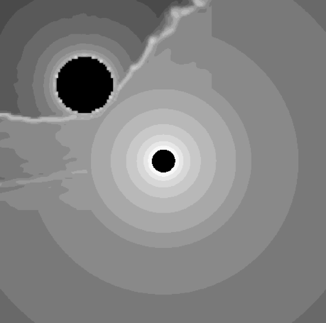
Figure 15: This figure shows the density distribution of the V444 Cyg model described in § 2.2.4. The density, including the bow shock, near the O star (upper-left) is from the hydrodynamical model of Pittard & Stevens (1999), and is added to the spherical density distribution of the W-R star (center) derived from a CMFGEN model. The parameters used in this model are: $R_{\mathrm{WR}}=4\,R_{\sun}$, $R_{\mathrm{O}}=10\,R_{\sun}$ and $a=38\,R_{\sun}$. $L_{\mathrm{WR}}=1.40\times 10^{5}\,L_{\sun}$, $L_{\mathrm{O}}=2.4\times 10^{5}\,L_{\sun}$, $\dot{M}_{\mathrm{WR}}=9.72\times 10^{-6}\,M_{\sun}\,\mathrm{yr}^{-1}$, $\dot{M}_{\mathrm{O}}=5.78\times 10^{-7}\,M_{\sun}\,\mathrm{yr}^{-1}$, $V^{\mathrm{WR}}_{\infty}=1800\,\mathrm{km}\,\mathrm{s}^{-1}$ and $V^{\mathrm{O}}_{\infty}=2900\,\mathrm{km}\,\mathrm{s}^{-1}$.

Figure 16: The light curves are computed with the parameters used in the hydrodynamical calculation of Pittard & Stevens (1999). They are: $R_{\mathrm{WR}}=4.0\,R_{\sun}$, $R_{\mathrm{O}}=10.0\,R_{\sun}$, $L_{\mathrm{WR}}=1.40\times 10^{5}\,L_{\sun}$, $L_{\mathrm{O}}=2.4\times 10^{5}\,L_{\sun}$, $\dot{M}_{\mathrm{WR}}=9.72\times 10^{-6}\,M_{\sun}\,\mathrm{yr}^{-1}$ and $\dot{M}_{\mathrm{O}}=5.78\times 10^{-7}\,M_{\sun}\,\mathrm{yr}^{-1}$. The solid lines are from the model without the bow shock and the O star wind. The dashed lines are the model with the O star wind and the bow shock from the hydrodynamical model of Pittard & Stevens (1999) (Fig. 15). No significant differences between the two models are seen in this figure.

In summary, from this analysis, we conclude that the mass-loss rate of the W-R star in V444 Cyg is $0.6\left(\pm 0.2\right)\times 10^{-5}\,M_{\sun}\,\mathrm{yr}^{-1}$. The size of the error in $\dot{M}$ is estimated from the light curves in Figs. 10 and 12. The mass-loss rate determined here is consistent with the values of STL2, and it is slightly higher than that of Underhill et al. (1990). (See Table 1 for other published values.) The range of the volume filling factor for the W-R star atmosphere is estimated to be $0.050-0.075$ with the corresponding range of the W-R star radius, $5.0-2.5\,R_{\sun}$. We also found that the presence of the bow shock, the exact details of the bow shock, and the presence of the O star wind are unimportant for the continuum fits, and they do not affect the mass-loss rate estimate given here.

3 Discussion

3.1 Infrared Light Curves

In order to check the consistency of our best fit models (Models B and E with $\dot{M}_{\mathrm{WR}}=0.6\times 10^{-5}\,M_{\sun}\mathrm{yr}^{-1}$) in § 2.2 with some other observational aspects, the infrared light curves (at $\lambda=2.2\,\mu\mathrm{m}$) were also computed. In order to calculate the IR light curves, the monochromatic luminosity ratio $q=L_{\mathrm{WR}}/L_{\mathrm{O}}$ at $\lambda=2.2\,\mu\mathrm{m}$ must first be estimated. In Model B, $q$ was determined to be $0.45$ at $\lambda=5630$ Å  in the previous section. By normalizing the O star flux with this value of $q$ at $\lambda=5630$ Å, $q$ for the wavelengths between $3000$ Å and $33,000$ Å is plotted in Fig. 17 for three different O star effective temperatures. The figure shows that the O star is brighter than the W-R star at $\lambda=5630$ Å, but the W-R star is brighter than the O star after $\lambda\sim 20,000$ Å. In model B, an O star temperature of $T_{\mathrm{O}}=35,000\,\mathrm{K}$ was used; hence, the corresponding value of $q$ at $\lambda=2.2\,\mu m$ is 1.10 according to the graph. For models with higher O star temperatures, the values of $q$ are slightly higher.

The resulting model IR light curves are shown in the right hand side of Figs. 10 and 12 along with Q and U polarization light curves for $\dot{M}_{\mathrm{WR}}=0.3\times 10^{-5}\,M_{\sun}$, $\dot{M}_{\mathrm{WR}}=0.6\times 10^{-5}\,M_{\sun}\,\mathrm{yr}^{-1}$ and $\dot{M}_{\mathrm{WR}}=1.2\times 10^{-5}\,M_{\sun}\,\mathrm{yr}^{-1}$. The figure also includes the observed IR light curve from the broadband ($K$) photometry obtained by Hartmann (1978). The depth of the primary eclipse (at $\phi=0$ or $1$ when the W-R star is in front of the O star) is fitted well for both $R_{\mathrm{WR}}=2.5\,R_{\sun}$ and $5.0\,R_{\sun}$ models, but the secondary eclipse modeled (at $\phi=0.5$ when the O star is in front of the W-R star) is shallower than the observed IR light curve. We also notice that the maximum $I$ flux level ($I_{\mathrm{max}}$) in the observed light curve is not well defined. Cherepashchuk et al. (1984) and Hamann & Schwarz (1992) had a similar problem – the primary and secondary eclipses are too shallow in their light curve model. While the light curve model of Hamann & Schwarz (1992) did not fit the depth of both eclipses, our model is consistent with at least the primary eclipse.

Cherepashchuk et al. (1984) discussed two possible causes for this problem: a). the existence of “third light” and b). the result of ignoring the reflection effect. They noted that one possible source of third light is the contribution of emission lines in the broad-band photometry at $2.2\,\mu\mathrm{m}$ as originally mentioned by Hartmann (1978), but we now expect this effect to be generally small (unless the He i $2.06\,\mu\mathrm{m}$ emission line is abnormally large). To examine this possibility, we have run a model which includes the reflection by the disk of the O star. However we find that it does not affect the infrared and optical light curves. Cherepashchuk et al. (1984) also conjectured that the increase in the depth and the width of the secondary eclipse (from optical to IR) is a result of clumps in the WR stellar wind.

If the wrong flux ratio at $\lambda=2.2\,\mu\mathrm{m}$ is used in our model, the secondary eclipse could become shallower at this wavelength. The differences in the depth of the secondary eclipse in Figs. 10 and 12 are approximately $8$% and $5$%. This could be explained by the wrong O star temperature used in the model. According to Fig. 17, $q$ at $2.2\,\mu\mathrm{m}$ also increases about $8$% if we use $T_{\mathrm{O}}=45,000\,\mathrm{K}$ although this would not fit the absorption components of the observed spectrum.

Figure 17: The continuum flux ratio $\left(q=F_{\mathrm{WR}}/F_{\mathrm{O}}\right)$ of Model B as a function of wavelength for three different O star effective temperatures. The lines were normalized at $\lambda=5630$Å  where the luminosity ratio $q=0.45$ was determined from the spectroscopic model fit (Fig. 9).

Table 3: Summary of the Best Fit Models

	Model B	Model E
$R_{\mathrm{WR}}\,\left[R_{\sun}\right]$	5.0	2.5
$R_{\mathrm{O}}\,\left[R_{\sun}\right]$	7.2	6.9
$\dot{M}_{\mathrm{WR}}$ $\left[\times 10^{-5}\,M_{\sun}\,\mathrm{yr}^{-1}\right]$	0.6	0.6
$f$	0.05	0.075
$q\left(\lambda 5630\right)$	0.45	0.31
$q\left(\lambda 22000\right)$	1.10	0.96
$i\,\left[\mathrm{deg}.\right]$	78.0	79.5
$M_{v}$ (O star)	-5.20	-4.85
$M_{v}$ (W-R star)	-4.33	-3.58
$M_{v}$ (O+W-R)	-5.60	-5.15
$m_{v}$ (O+W-R)$\left(*\right)$	8.38	8.84
$DM$ $\left(**\right)$	11.1	10.6

$\left(*\right)$ Assuming a distance of 1.7 kpc and $E_{b-v}=0.68$ Lundström & Stenholm (1984) – They assumed the intrinsic color to be $\left(b-v\right)_{o}=-0.30$.

$\left(**\right)$ Using the observed value of $m_{v}=8.27$ and $A_{v}=2.79$ from Lundström & Stenholm (1984).

3.2 Polarization Curves near the Secondary Eclipse

In both Model B (Fig. 10) and Model E (Fig. 12), the amplitude of the $U$ polarization variation near the secondary eclipse ($\phi=0.5$) underestimates the observed level. A larger polarization amplitude can be obtained if the radius of the O star is increased, although this will result in an inconsistent depth of the secondary eclipse. A possible cause of this inconsistency is the inaccurate stellar wind structure very close to the core of the W-R star. For all the models in Table 2, $\beta_{1}=1$ was used in the modified beta-velocity law (Hillier & Miller 1999) (see Eq. 1) where $\beta_{1}$ is equivalent to $\beta$ in the classic beta-velocity law for the “inner” part of the stellar wind. To see if changing the structure of the inner W-R stellar wind affects the computed continuum polarization level, a model with $\beta_{1}=2$ (a slower wind) is also calculated. Unfortunately, the amplitude of the polarization curves (not shown here) near $\phi=0.5$ did not change significantly for the new $\beta_{1}$ value. Changing the value of $\beta_{1}$ also did not influence the depth of the secondary eclipse in the IR light curve.

We note that STL2 were able to fit the observed $Q$ and $U$ variations around $\phi=0.5$. There are two reasons for their success: 1. they did not fit the observed $I$ light curve consistently, and 2. they use a fixed orbital inclination angle. In their fitting procedure, the radius of the O star was used as a fitting parameter, but changing the O star radius changes the depth of the eclipse around $\phi=0.5$. Consequently, the inclination angle must also be adjusted when the O star radius is changed, to maintain a consistency with the observed $I$ light curve. We should also note that the amplitudes of polarization curves around $\phi=0.5$ are very sensitive to the orbital inclination. STL2 adopted $i=78.9^{\circ}$ from Robert et al. (1990). However, if instead $i=78^{\circ}$ from Cherepashchuk (1975) were used, they would obtain a fairly different set of parameters from the ones derived in their paper. Fortunately, the amplitudes of the double sine curves are not very sensitive to the adopted inclination angle. Considering the relative sensitivity of different methods on the inclination angle, the mass-loss rate estimation by fitting the double sine curves is more reliable than the one obtained by fitting the polarization variations near $\phi=0.5$.

3.3 Magnitudes and Distance Moduli

For each model in Figs. 10 and 12, the absolute magnitude ($M_{v}$) of the system (W-R + O) is calculated, and placed in Table 3. $M_{v}=-5.60$ from Model B is very similar to $M_{v}=-5.7$ of Lundström & Stenholm (1984), but is far from the value of Hamann & Schwarz (1992), $M_{v}=-4.2$. Model E gives $M_{v}=-5.15$ which is slightly different from the values estimated by Lundström & Stenholm (1984) and Hamann & Schwarz (1992). Using the observed $m_{v}=8.27$ and $A_{v}=2.79$ from Lundström & Stenholm (1984), we have also estimated the distance modulus ($DM$) for each model, and summarized them in the same table. The values of $DM$ from Model B and Model E are $11.1$ and $10.6$ respectively. The former (Model B) agrees with the value given by Lundström & Stenholm (1984) ($DM=11.01\pm 0.20$), but it is slightly smaller than the value estimated by Marchenko et al. (1997) ($DM=11.27-11.47$).

The absolute magnitudes of the O star corresponding to Models B and E are also listed in Table 3. They are $M_{v}=-5.20$ and $M_{v}=-4.85$ respectively. According to Howarth & Prinja (1989), the mean absolute magnitude of O6 V stars is $M_{v}=-5.2$, and that for O6 III is $M_{v}=-6.6$. Our magnitude of Model B agrees with the mean of their O6 V stars. Similarly, the average absolute magnitude of observed WN5 stars is $M_{v}=-4.1\left(\pm 0.8\right)$ (van der Hucht 2001) which also agrees with our values $M_{v}=-4.33$ (Model B) and $M_{v}=-3.58$ (Model E).

The derived O star radii are $R_{\mathrm{O}}=7.2\,R_{\sun}$(Model B) and $R_{\mathrm{O}}=6.9\,R_{\sun}$(Model E). Both values are slightly smaller than the recent value $R_{O}=8.5\pm 1.0\,R_{\sun}$ estimated by STL2, and are not consistent with $R_{\mathrm{O}}=10.0\,R_{\sun}$ (Cherepashchuk et al. 1984) and $R_{\mathrm{O}}=8.4-9.3\,R_{\sun}$ (Moffat & Marchenko 1996). The rather small O star radii of the models and the model $M_{v}$ values compared to the mean observed $M_{v}$ suggest that the O star is more likely to be a main-sequence star rather than a giant star. A similar conclusion about the O star luminosity class was reached by STL2.

Vanbeveren et al. (1998) quoted Cherepashchuk (1975), ”The observed mass of the WNE component is $9\,M_{\sun}$; its progenitor must therefore have had a mass of $\sim 30\,M_{\sun}$. Thus, the age of the binary is about 7 million years. The OB companion is an O6 star. Since the age of a normal O6 star is about 1-2 million years, the OB star must have been rejuvenated, i.e. mass transfer must have occurred.” This argument suggests that the O star is not a normal O star. According to Vanbeveren et al. (1998), a quasi-conservative Roche lobe overflow model can produce a system which resembles V444 Cyg. At the end of the mass transfer, when the secondary has been entirely mixed, the O6 component may be an over-luminous star with $M_{\mathrm{O}}=26\,M_{\sun}$. Contrary to the last remark, our best fit models (Models B and E) suggest that the absolute magnitude of the O star is similar to the average of O6 V stars, as discussed earlier.

Unfortunately, we can not strongly conclude that either Model B or E is a more favorable model based on the comparisons with the observed magnitudes, distance moduli and the results from earlier works.

4 Conclusions

Using the 3-D Monte Carlo model developed in Paper I, combined with the multi-line non-LTE radiative model of Hillier & Miller (1998), we first investigated the basic behavior of the WN star diagnostic lines (He ii $5412$ Å and He i $5876$ Å) as a function of the phase of V444 Cyg (Figs. 4–6). Since the emission lines from the W-R star envelope are contaminated by the O star atmospheric absorption lines and the line emission from the shock-heated region, we first examined at which phase the profile shape of helium lines, especially He i $5876$ Å, is least affected by the contaminations. We then fit the He i $5876$ Å profile with the multi-line non-LTE radiative transfer model with spherical geometry to obtain a realistic model for the W-R star. The best orbital phase for this purpose is found to be around $\phi=0.8$.

A summary of the derived parameters of V444 Cyg with our best fit models (Models B & E) is given in Table 3. Both models show excellent agreement with the observed light curves of $I$, $Q$ and $U$ Stokes parameters (Figs. 10 and 12). They also fit the spectrum of He ii $5412$ Å and He i $5876$ Å very well (Figs. 9 and 11). The effect of ignoring the presence of the bow shock in the continuum polarization calculation was also considered. This was done by first approximating the opacity in the bow shock region via fitting He i $5876$ Å line at $\phi=0.419$ where the emission from the bow shock is most prominent (Fig 13). According to this model, the bow shock region has little or no effect on the continuum light curves at $\lambda=5630$Å for all $I$, $Q$ and $U$ (Fig. 14). Similarly, the presence of the O-star wind and the exact details of the bow shock are found to be unimportant for the continuum fits (Fig. 16). We also found that the spectroscopic solution, when combined with the strong O star spectrum, is very insensitive to the value of the W-R core radius (c.f., Fig. 9 and Fig. 11).

Small discrepancies are seen in the oscillation of the $Q$ and $U$ light curves (Figs. 10 and 12) near the secondary eclipse ($\phi=0.5$), which are possibly due to the lack of knowledge of the exact opacity and emissivity in the bow shock region. This discrepancy could be a result of the wrong combination of the orbital inclination angle and the O star radius in our model. The shape of the polarization curves near $\phi=0.5$ is very sensitive to the inclination angle, and is difficult to fit consistently with other observational features.

The most noticeable difference between our best model and the observations is in the IR light curves ($2.2\,\mu\mathrm{m}$) in Figs. 10 and 12. The model correctly predicts the depth of the primary eclipse, but that of the secondary eclipse is too shallow. We argued that the difference could be caused by the use of the wrong monochromatic luminosity ratio ($q$) at $\lambda=2.2\,\mu\mathrm{m}$.

The mass-loss rate of the W-R component determined in our analysis is $\dot{M}_{\mathrm{WR}}=0.6\left(\pm 0.2\right)\times 10^{-5}\,M_{\sun}\,\mathrm{yr}^{-1}$, and this conclusion is insensitive to the model radius of the W-R star. The mass-loss rate of the W-R star obtained by STL2, $\dot{M}_{\mathrm{WR}}=0.6\times 10^{-5}\,M_{\sun}\,\mathrm{yr}^{-1}$, is in good agreement with our value derived here. Our derived mass-loss rate lies between the values obtained by the orbital period change method (Table 1). The fits did not allow a unique value for the radius of the W-R star to be derived. The range of the volume filling factor for the W-R star atmosphere is estimated to be $0.050-0.075$ for the corresponding range of the W-R star radius, $5.0-2.5\,R_{\sun}$.

Future work includes: 1. obtaining improved IR light curves for both models and observations, 2. fitting and modeling the UV spectrum and polarization, 3. checking the consistency between the polarization model and the hydrodynamical model more carefully, 4. investigating the cause for the asymmetry of the polarization light curve around the secondary eclipse, and 5. obtaining a tighter constraint on $q$. Future interferometer observations of this system will also prove invaluable to our further understanding.