Measured Mass Loss Rates of Solar-like Stars as a Function of Age and Activity

Abstract

Collisions between the winds of solar-like stars and the local ISM result in a population of hot hydrogen gas surrounding these stars. Absorption from this hot H I can be detected in high resolution Ly$\alpha$ spectra of these stars from the Hubble Space Telescope. The amount of absorption can be used as a diagnostic for the stellar mass loss rate. We present new mass loss rate measurements derived in this fashion for four stars ($\epsilon$ Eri, 61 Cyg A, 36 Oph AB, and 40 Eri A). Combining these measurements with others, we study how mass loss varies with stellar activity. We find that for the solar-like GK dwarfs, the mass loss per unit surface area is correlated with X-ray surface flux. Fitting a power law to this relation yields $\dot{M}\propto F_{x}^{1.15\pm 0.20}$. The active M dwarf Proxima Cen and the very active RS CVn system $\lambda$ And appear to be inconsistent with this relation. Since activity is known to decrease with age, the above power law relation for solar-like stars suggests that mass loss decreases with time. We infer a power law relation of $\dot{M}\propto t^{-2.00\pm 0.52}$. This suggests that the solar wind may have been as much as 1000 times more massive in the distant past, which may have had important ramifications for the history of planetary atmospheres in our solar system, that of Mars in particular.

1 INTRODUCTION

The existence of a mass outflow from the Sun has been recognized for many decades, its presence revealed most visibly by the behavior of comet tails (e.g., Biermann, 1957). It has also been recognized for many years that the solar wind has its origin in the Sun’s hot corona. Thus, it is expected that all cool stars with analogous hot coronae will have similar winds (e.g., Parker, 1960).

Nevertheless, actually detecting a solar-like wind emanating from another star has proved to be very difficult. This is perhaps not surprising given that the solar wind itself is not particularly easy to observe remotely. The low density of the wind, corresponding to a mass loss rate of only $\dot{M}_{\odot}=2\times 10^{-14}$ M_⊙ yr^-1 (e.g., Feldman et al., 1977), and its high temperature and ionization state make it difficult to detect with simple imaging or spectroscopic techniques. Trying to detect such a wind around another star is needless to say even more daunting. This is in contrast to the massive winds of hot stars and evolved cool stars, which are comparatively easy to detect spectroscopically thanks to the characteristic P-Cygni line profiles that signify the presence of these strong winds.

Fortunately, a method for indirectly detecting solar-like stellar winds has recently become available using high resolution Hubble Space Telescope (HST) spectra of the H I Ly$\alpha$ lines from nearby stars. The method is indirect because the material that is detected in Ly$\alpha$ absorption is not from the wind itself, which is fully ionized and therefore has no H I, but is instead interstellar H I that is heated within the interaction region between the wind and the local interstellar medium (LISM). The existence of this detectable hot H I was first suggested by hydrodynamic models of our own heliosphere, which describe how the radial solar wind interacts with the laminar interstellar wind seen from the Sun’s rest frame (Baranov & Malama, 1993, 1995; Pauls, Zank, & Williams, 1995; Zank et al., 1996; Baranov, Izmodenov, & Malama, 1998; Zank, 1999).

The plasma collisions between the fully ionized solar wind and partially ionized LISM establish the familiar large scale structure of the heliosphere, consisting of three discontinuities in the flow: the termination shock where the solar wind is shocked to subsonic speeds, the heliopause separating the plasma flows of the wind and the LISM, and the bow shock where the interstellar wind is shocked to subsonic speeds. The distances to these boundaries in the upwind direction are currently estimated to be roughly 85, 125, and 240 AU for the termination shock, heliopause, and bow shock, respectively. The Voyager 1 and Voyager 2 spacecraft are currently 82 and 65 AU away, respectively, more or less in the upwind direction, so hopefully they will soon cross the termination shock and observationally establish its true location.

The LISM is only partially ionized, but including the neutral LISM component in models of the heliosphere is difficult, because the charge exchange processes that allow the H I to take part in the wind-LISM interaction force the H I out of thermal and ionization equilibrium. It is only relatively recently that codes including neutrals in a self-consistent manner have been developed (Baranov & Malama, 1993, 1995; Pauls et al., 1995; Zank et al., 1996). It is these models that show that our heliosphere should be permeated by H I with an effective temperature of $T\sim 20,000-40,000$ K, much of which is piled up between the heliopause and bow shock, creating a so-called “hydrogen wall.” It is this hot H I that produces a Ly$\alpha$ absorption signature broad enough to be at least partially separable from the absorption of the cooler LISM material ($T\approx 8000$ K).

This hot heliospheric H I was first detected in Ly$\alpha$ observations of $\alpha$ Cen A and B (Linsky & Wood, 1996; Gayley et al., 1997), where it was shown that the ISM alone could not account for the observed H I absorption, and that the excess absorption on the red side of the line was consistent with the heliospheric H I absorption predicted by the heliospheric models. The heliospheric absorption is redshifted relative to the ISM due to the deceleration of ISM material as it crosses the bow shock. The heliospheric models could not, however, account for the observed excess on the blue side of the line, which Gayley et al. (1997) attributed to analogous “astrospheric” H I surrounding $\alpha$ Cen A and B. This interpretation was confirmed by observations of $\alpha$ Cen’s distant companion Proxima Cen, which show that the blue side excess is not seen toward Proxima Cen, proving that the blue side excess absorption seen toward $\alpha$ Cen must be due to circumstellar material around $\alpha$ Cen that does not extend as far as the distant companion Proxima Cen (Wood et al., 2001). In the meantime, astrospheric absorption was also detected toward several other nearby cool stars: $\epsilon$ Ind and $\lambda$ And (Wood, Alexander, & Linsky, 1996); $\epsilon$ Eri (Dring et al., 1997); 61 Cyg A and 40 Eri A (Wood & Linsky, 1998); and 36 Oph (Wood, Linsky, & Zank, 2000a). However, the 40 Eri A and $\lambda$ And detections must be regarded as tentative and require confirmation.

These detections of astrospheric H I represent the first detections, albeit indirect, of solar-like winds around other stars. Detecting solar-like stellar winds is important for many reasons. By observing solar phenomena such as the solar wind on other stars, we can in principle improve our understanding of these phenomena in ways that are impossible based on observations of the Sun alone. For example, the extensively studied correlation between rotation and stellar magnetic activity reveals the importance of rapid rotation in the generation of high activity levels in stars (Pallavicini et al., 1981; Walter, 1982, 1983; Caillault & Helfand, 1985; Micela et al., 1985; Fleming, Gioia, & Maccacaro, 1989; Stauffer et al., 1994; Ayres, 1997). The rotation/activity correlation provides valuable information about the dynamo mechanism that produces magnetic activity on the surfaces of cool stars, including the Sun, but this information can only be acquired by observing stars with different rotation rates. Similarly, our understanding of the acceleration mechanisms of solar-like winds could in principle be improved significantly by measurements of how wind properties differ for different types of cool stars. Since winds play a crucial role in the magnetic braking process that slows stellar rotation with time, measuring wind properties of stars with different ages could also improve our understanding of stellar angular momentum evolution.

However, in order for these benefits to be realized, the astrospheric analyses must not only yield detections of stellar winds but also measurements of their properties. Fortunately, the amount of astrospheric absorption is dependent on the stellar mass loss rate, since larger mass loss rates will yield larger astrospheres and therefore larger column densities. With the assistance of hydrodynamic models, Wood et al. (2001) demonstrated that the astrospheric absorption observed toward $\alpha$ Cen suggests a mass loss rate of $\dot{M}=2~{}\dot{M}_{\odot}$ for the combined winds of $\alpha$ Cen A and B (both stars lie within the same astrosphere), and an upper limit of $\dot{M}<0.2~{}\dot{M}_{\odot}$ for Proxima Cen. Müller, Zank, & Wood (2001a) presented estimates for the mass loss rates of $\epsilon$ Ind and $\lambda$ And, which were revised by Müller, Zank, & Wood (2001b) based on additional modeling to $\dot{M}=0.5~{}\dot{M}_{\odot}$ for $\epsilon$ Ind and $\dot{M}=5~{}\dot{M}_{\odot}$ for $\lambda$ And. In this paper, we estimate mass loss rates for the other stars with detected astrospheric absorption ($\epsilon$ Eri, 61 Cyg A, 40 Eri A, and 36 Oph). Preliminary results of this analysis were presented by Wood et al. (2002). Finally, we consider all the mass loss measurements together to see what they suggest about how mass loss varies with activity and spectral type.

2 MEASURING MASS LOSS RATES

2.1 The Sample of Stars with Detected Astrospheres

The seven stars with detected astrospheric absorption are listed in Table 1, along with their spectral types and Hipparcos distances (Perryman et al., 1997). Also listed is Proxima Cen, for which an upper limit for astrospheric absorption yields an upper limit for its mass loss rate (Wood et al., 2001). In some binary systems, both stars will lie within the same astrosphere, meaning the astrospheric absorption will be characteristic of the combined mass loss of both stars. This is the case for the $\alpha$ Cen, 36 Oph, and $\lambda$ And systems (see Table 1), while 61 Cyg A and 40 Eri A will have astrospheres all to themselves despite being members of multiple star systems (see §2.4–2.6).

The surface areas listed in Table 1 (in solar units) are the combined surface areas of all stars within the detected astrospheres. Most of these areas are based on stellar radii computed using the Barnes-Evans relation (Barnes, Evans, & Moffett, 1978), except for Proxima Cen and $\lambda$ And, for which we assume radii of 0.16 R_⊙ and 7.4 R_⊙, respectively (Panagi & Mathioudakis, 1993; Nordgren et al., 1999). The activity level of the stars is indicated in Table 1 by their X-ray luminosities, $L_{x}$, in units of ergs s^-1. These luminosities are based on ROSAT PSPC data. Most of the $\log L_{x}$ values are from Hünsch et al. (1999), with the exception of the $\lambda$ And luminosity, which is from Ortolani et al. (1997). Following Schmitt, Fleming, & Giampapa (1995), we assume that 61 Cyg A contributes 64% of the binary’s X-ray flux.

In order to use the observed amount of astrospheric absorption to derive a mass loss rate, it is first necessary to estimate the interstellar wind velocity seen by each star ($V_{ISM}$) and the orientation of the astrosphere relative to the line of sight, which can be described by the angle between the upwind direction and the line of sight ($\theta$). Two velocity vectors must be known in order to compute these quantities, that of the interstellar flow and that of the star itself. Since all the stars in Table 1 are very nearby, their proper motions, radial velocities, and thus their stellar vectors are known very well.

For most of the stars, we simply use the velocity vector of the Local Interstellar Cloud (LIC) from Lallement et al. (1995) to represent the ISM flow at the location of the star. Two exceptions are the Alpha/Proxima Cen and 36 Oph systems, which lie not within the LIC but within the “G cloud,” which has a vector measured by Lallement & Bertin (1992). The G cloud vector is, however, very similar to the LIC vector, so its use results only in minor modifications to the $V_{ISM}$ and $\theta$ values. A few of the stars in Table 1 lie in neither the LIC or G clouds. The 61 Cyg system clearly falls in this category based on the two-component velocity structure seen for this line of sight (Wood & Linsky, 1998), and the $\lambda$ And system is much too far away to be within the LIC or G clouds. However, even when multiple ISM components are detected within the LISM, they are generally separated by no more than $5-10$ km s^-1, meaning the LIC vector should be a reasonable approximation for these other nearby clouds, much as it is for the G cloud. In any case, the $V_{ISM}$ and $\theta$ values for all stars in our sample are listed in Table 1. The $V_{ISM}$ values can be compared with the solar value of 26 km s^-1 suggested by the LIC vector.

Note that two of the astrospheric detections have been flagged as being uncertain in Table 1. The $\lambda$ And detection is uncertain because there are no observations of narrow ISM lines such as Mg II h & k to provide information on the velocity structure of the ISM for that line of sight. As a consequence, the H I and D I (deuterium) Ly$\alpha$ lines are analyzed assuming a single absorption component. This analysis clearly suggests the presence of excess H I absorption on the blue side of the line that Wood et al. (1996) interpret as astrospheric absorption, but without knowledge of the ISM velocity structure it remains possible that there is a blueshifted ISM component that might be able to account for the H I excess without requiring an astrospheric component. The 40 Eri A detection is also flagged as uncertain for reasons that will be discussed in §2.6.

The third-to-last column of Table 1 lists the column density of the hot astrospheric H I based on the best astrospheric model fit to the data, and the next column is the mass loss rate assumed for this best model. Finally, the last column lists references relating to the detection of the astrospheric absorption and from it the measurement of the mass loss rate. However, as noted in §1, mass loss rates for four of the stars ($\epsilon$ Eri, 61 Cyg A, 40 Eri A, and 36 Oph) are measured for the first time in this paper. Thus, we now describe in detail how we make these measurements.

2.2 Astrospheric Modeling

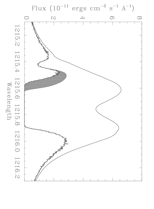
Figure 1: HST/GHRS Ly$\alpha$ spectrum of $\epsilon$ Eri, showing broad H I absorption at 1215.7 Å and narrow D I absorption at 1215.4 Å. The upper solid line is the assumed intrinsic stellar emission line, and the dotted line is the profile after ISM absorption alone, derived by forcing consistency between the ISM H I and D I absorption. The excess H I absorption on the blue side of the line (shaded region) is astrospheric absorption.

One of the best examples of astrospheric absorption is that observed toward $\epsilon$ Eri. Figure 1 shows the Ly$\alpha$ profile of $\epsilon$ Eri observed by the Goddard High Resolution Spectrograph (GHRS) instrument on HST. Like all such profiles, the center of the emission line is absorbed by a very broad H I absorption feature flanked by a much narrower absorption feature from interstellar D I, $-0.33$ Å from the H I absorption.

The upper solid line in Figure 1 is an estimate of the original stellar Ly$\alpha$ emission profile. Uncertainty in the stellar Ly$\alpha$ profile is the dominant source of systematic error in the analysis of the H I absorption for all the stars in Table 1. Thus, a major goal of the empirical analyses referenced in Table 1 is to experiment with different profiles to make sure that results are not dependent on the assumed profile. The Mg II h & k line profiles (at 2803.531 Å and 2796.352 Å, respectively) are sometimes used as guides for how the stellar profiles should appear, since the Ly$\alpha$ and Mg II lines are both highly optically thick chromospheric lines and the solar Ly$\alpha$ and Mg II profiles are known to be quite similar. This is why most of the profiles for the stars in Table 1 are assumed to have self-reversals near line center, like that for $\epsilon$ Eri in Figure 1, although results of the H I absorption fitting are never very sensitive to the exact depth or shape of the self-reversal. Some analyses also force the wings of the Ly$\alpha$ line to be centered on the rest frame of the star, which can be a useful constraint in certain circumstances (Wood & Linsky, 1998; Wood et al., 2000a). We refer the reader to the references listed in Table 1 for details about each particular analysis, but considering possible alterations to assumed stellar profiles is also necessary here in deciding if an astrospheric model is consistent with the data or not (see below and §2.6).

The dotted line in Figure 1 is the profile after ISM absorption alone, which is derived by fitting the Ly$\alpha$ absorption profile while using the D I absorption to constrain the properties of the H I absorption. The centroid velocity of the H I absorption is forced to be the same as that of the D I absorption, and since H I and D I lines in the LISM are thermally broadened, the Doppler broadening parameters of the H I and D I absorption can also be related by $b(H~{}I)=\sqrt{2}b(D~{}I)$ (see, e.g., Linsky & Wood, 1996; Wood & Linsky, 1998; Wood et al., 2000a). With these sensible constraints, it becomes immediately obvious that the H I absorption is inconsistent with the D I absorption. In particular, it is too broad and blueshifted relative to D I. Thus, there is a large excess of absorption on the blue side of the H I absorption that cannot be explained by ISM absorption (Dring et al., 1997).

Hydrodynamic models of the heliosphere suggest that heliospheric H I absorption should be redshifted relative to the ISM absorption regardless of whether the line of sight is upwind, downwind, or sidewind. This is primarily due to the deceleration and deflection of interstellar material as it crosses the bow shock, although other factors are at work downwind (Izmodenov, Lallement, & Malama, 1999; Wood, Müller, & Zank, 2000b). Conversely, astrospheric absorption should generally be blueshifted relative to the ISM absorption, since we are observing the absorption from outside the astrosphere rather than inside. All of the excess absorption observed toward $\epsilon$ Eri is on the blue side of the line, suggesting that the stellar astrosphere is responsible for the excess rather than our heliosphere.

To quantitatively measure mass loss rates based on astrospheric absorption like that seen for $\epsilon$ Eri in Figure 1 requires the use of hydrodynamic models of the astrosphere. However, it is crucial that these astrospheric models be extrapolated from a heliospheric model that has been demonstrated to successfully reproduce heliospheric H I absorption. Essentially, the heliospheric H I absorption is used to calibrate the models before applying them to the case of astrospheres.

Excess H I absorption on the red side of the Ly$\alpha$ line that can be interpreted as heliospheric in origin has been clearly detected toward three different stars: $\alpha$ Cen (Linsky & Wood, 1996), 36 Oph (Wood et al., 2000a), and Sirius (Izmodenov et al., 1999). There are more subtle suggestions of some heliospheric contribution to the H I absorption observed toward Capella and G191-B2B, which are very similar lines of sight (Vidal-Madjar et al., 1998; Lemoine et al., 2002). Wood et al. (2000b) compare the heliospheric absorption observed for the first three lines of sight listed above (and upper limits for heliospheric absorption provided by three other lines of sight) with the predictions of many heliospheric models. Two different codes are used, a “Boltzmann” code that uses a kinetic treatment of the neutrals (Müller, Zank, & Lipatov, 2000), and a “four-fluid” code that models the heliosphere as an interaction involving four distinct fluids: a plasma component and three neutral components (Zank et al., 1996). The three neutral components represent the three distinct regions within the heliosphere where charge exchange occurs, which are separated by the heliopause and termination shock boundaries.

The solar wind parameters that must be assumed for these models are the wind velocity ($V_{w}$), proton density ($n_{w}(H^{+})$), and temperature ($T_{w}$) at 1 AU; which are assumed to be $V_{w}=400$ km s^-1, $n_{w}(H^{+})=5$ cm^-3, and $T_{w}=10^{5}$ K. These values are within the observed range of solar wind properties at Earth (e.g., Feldman et al., 1977). Note that the actual solar wind varies with time and ecliptic latitude, with $n_{w}(H^{+})=3$ cm^-3 and $V_{w}=750$ km s^-1 being more typical at high latitudes (McComas et al., 2001). The interstellar parameters that must be assumed include the ISM wind velocity ($V_{ISM}$), proton density ($n_{ISM}(H^{+})$), H I density ($n_{ISM}(H~{}I)$), and temperature ($T_{ISM}$). The velocity $V_{ISM}=26$ km s^-1 is known very well for the Sun, but the other ISM parameters can be varied within their various observational tolerances (see Wood et al., 2000b). Wood et al. (2000b) also experiment with various values for a parameter increasing the ISM pressure in order to account for the highly uncertain magnetic and cosmic ray pressure within the ISM. Despite experimentation with different input parameters, no Boltzmann model was found that could adequately reproduce the heliospheric H I absorption for all the lines of sight mentioned above. However, a four-fluid model that assumes $n_{ISM}(H^{+})=0.1$ cm^-3, $n_{ISM}(H~{}I)=0.14$ cm^-3, $T_{ISM}=8000$ K, and no correction for ISM magnetic field or cosmic ray pressure accurately reproduces the heliospheric absorption.

Thus, we use this model as the starting point for our astrospheric modeling. This model is a $\dot{M}=1~{}\dot{M}_{\odot}$ model appropriate for a $V_{ISM}=26$ km s^-1 system. In order to construct a $\dot{M}=2~{}\dot{M}_{\odot}$ model for $\epsilon$ Ind, for example, we would compute another four-fluid model with $n_{w}(H^{+})$ increased by a factor of 2 to $n_{w}(H^{+})=10$ cm^-3 and with the ISM wind speed changed to the $V_{ISM}=68$ km s^-1 value appropriate for $\epsilon$ Ind (see Table 1). All other parameters are kept the same.

This assumes that ISM parameters do not vary greatly from location to location within the LISM. This assumption is a source of systematic error for our analysis, and we note that Frisch (1993) actually proposed using astrospheric properties as probes of the ISM rather than using astrospheres as diagnostics for the stellar winds. However, if different regions of the LISM are in pressure equilibrium, LISM properties should not vary too severely. Furthermore, Izmodenov, Lallement, & Wood (2002) find that their models suggest surprisingly low sensitivity of astrospheric H I absorption to changes in the assumed ISM densities, at least in upwind and sidewind directions, meaning that modest variations in LISM densities should not greatly prejudice our results.

The inaccuracies and different approximations in current heliospheric/astrospheric models are such that different types of models developed by different groups can be expected to predict somewhat different properties and different amounts of H I absorption, even if the models all assume the same input parameters (Baranov et al., 1998; Wood et al., 2000b). This is why it is so important to extrapolate the astrospheric models from a heliospheric model that successfully reproduces the observed heliospheric H I absorption. If, for example, we were to find a heliospheric Boltzmann model that reproduced the observed heliospheric H I absorption, it would likely have different input ISM parameters than those that worked for the four-fluid code. However, this does not necessarily mean that stellar mass loss rates derived from Boltzmann models will be significantly different from those derived here using the four-fluid code, as long as the astrospheric Boltzmann models are extrapolated from the successful heliospheric model, assuming the ISM input parameters that worked for that model rather than the parameters that worked for the successful four-fluid heliospheric model. All types of models that currently exist should have the property that larger mass loss rates will yield increasing amounts of H I absorption. Thus, if all types of codes are first calibrated by demonstrating that a $\dot{M}=1~{}\dot{M}_{\odot}$, $V_{ISM}=26$ km s^-1 model reproduces the observed heliospheric H I absorption, much of the potential model dependence can be removed.

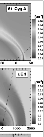
Figure 2: Maps of H I density from hydrodynamic models of stellar astrospheres. The models shown are the ones that lead to the best fits to the data in Fig. 3. The distance scale is in AU. The star is at coordinate (0,0) and the ISM wind is from the right. The dashed lines indicate the Sun–star line of sight.

Figure 2 shows examples of various astrospheric models constructed for various stars in our sample. These are in fact the models that yield the best fits to the data, as we will show below. The figure shows the H I density distribution. In each panel, the high density area in red between the bow shock and heliopause is the so-called hydrogen wall that is responsible for most of the astrospheric absorption for all of these lines of sight. The models also provide distributions of H I temperature and flow velocity. From these distributions, we can trace out the H I density, temperature, and flow velocity along the line of sight to the star, which is indicated by the $\theta$ values in Table 1 and shown explicitly in Figure 2. And from these tracings we can determine the predicted H I absorption based on the model. We assume that nonthermal velocities do not contribute significantly to the line broadening. This seems a safe assumption given that for the astrospheric models in Figure 2, the high temperatures of the hot astrospheric H I lead to very large Doppler broadening parameters of $b=15-45$ km s^-1, meaning turbulence would have to be extreme to increase them even further. Nonthermal broadening is known to be insignificant for H I in the LISM, where temperatures are lower (e.g., Wood & Linsky, 1998).

Technically, Figure 2 shows the H I distribution for only the most important of the three H I components used in the four-fluid code, the “Component 1” neutrals (see Zank et al., 1996), which include the undisturbed LISM H I and H I created by charge exchange with heated LISM protons in the hydrogen wall. The other two components are H I particles created by charge exchange with the very hot, decelerated solar wind protons in between the termination shock and heliopause (“Component 2”), and H I created by charge exchange with the cold, fast solar wind protons within the termination shock (“Component 3”). We sum the absorption from all three components before a final absorption profile is derived for the model.

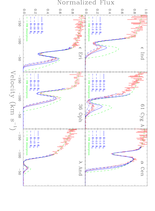
Figure 3: Closeups of the blue side of the H I Ly$\alpha$ absorption lines for all stars with detected astrospheric absorption, plotted on a heliocentric velocity scale. Narrow D I ISM absorption is visible in all the spectra just blueward of the saturated H I absorption. Green dashed lines indicate the interstellar absorption alone, and blue lines in each panel show the additional astrospheric absorption predicted by hydrodynamic models of the astrospheres assuming various mass loss rates.

By constructing different models with different assumed mass loss rates, as described above, we can obtain predicted Ly$\alpha$ absorption profiles for a range of mass loss rates to compare with the data. This comparison is made in Figure 3 for six of the stars in our sample. Three of the data-model comparisons in Figure 3 and best-fit models in Figure 2 ($\epsilon$ Ind, $\alpha$ Cen, and $\lambda$ And) are actually from previous work (Wood et al., 2001; Müller et al., 2001b), which we show here for purposes of comparison. The other three stars shown (61 Cyg A, $\epsilon$ Eri, and 36 Oph) are new analyses. We focus on the blue side of the H I Ly$\alpha$ absorption feature in Figure 3, since that is where the astrospheric absorption is most apparent. Each panel shows the ISM absorption alone (green dashed line), derived from previous empirical analyses (see references listed in Table 1) by forcing the H I absorption to be consistent with the D I absorption, which is also visible in the figure. In all cases there is a substantial amount of excess absorption that we interpret as astrospheric. The H I absorption predictions of astrospheric models are shown as blue lines in each panel. Table 1 lists the mass loss rates that we believe lead to the best matches to the data.

In principle, discrepancies between the models and the data seen in Figure 3 can be reduced if changes are made to the assumed stellar Ly$\alpha$ profiles. An example of this will be given in §2.6 for 40 Eri A. However, it is difficult to shift the location where the H I absorption becomes saturated by any reasonable change to the stellar profile. Trying to correct discrepancies at the base of the absorption typically results in the introduction of unreasonable fine structure into the assumed stellar line profile (Wood et al., 2000b). Thus, the base of the H I absorption (e.g., at $-50$ km s^-1 for $\epsilon$ Ind or $-25$ km s^-1 for $\epsilon$ Eri in Fig. 3) is less affected by uncertainties in the stellar profile than the upper part of the H I absorption profile, so the base of the profile is the best place to compare the data and the models when deciding which model is the best fit. For this reason, we consider the best fit to the $\epsilon$ Ind data to be the $0.5~{}\dot{M}_{\odot}$ model rather than the $0.8~{}\dot{M}_{\odot}$ model (see Fig. 3).

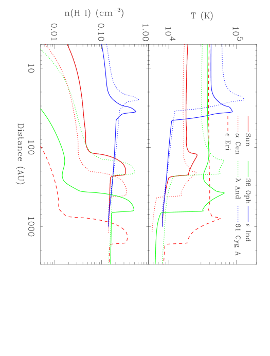
Figure 4: Variation of the H I temperature and density with distance from the star in the upwind direction ($\theta=0^{\circ}$) based on the “best-fit” models in Fig. 2, and on the best solar model from Wood et al. (2000b).

Figure 2 illustrates the large range of size scales that the astrospheres have. This is illustrated more directly in Figure 4, where we show the variations of H I density and temperature with distance from the star in the upwind direction (i.e., $\theta=0^{\circ}$) for these models and the best solar model from Wood et al. (2000b). Stars with faster $V_{ISM}$ speeds (e.g., $\epsilon$ Ind and 61 Cyg A; see Table 1) have hotter astrospheric H I due to more heating at the bow shock. Their astrospheres also tend to be more compact, and the density enhancements within the hydrogen wall somewhat larger. Stars with larger mass loss rates naturally tend to have larger astrospheres.

We now discuss some aspects of the mass loss derivations for each particular star separately, at least for the new analyses presented here.

2.3 $\epsilon$ Eridani

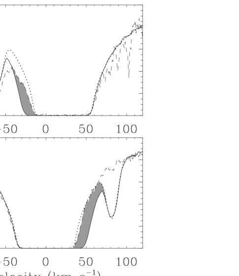
Figure 5: (a) The observed H I Ly$\alpha$ line of $\epsilon$ Eri (solid line) and the Ly$\alpha$ profile with only ISM absorption (dotted line) for $\epsilon$ Eri from Fig. 1 are compared with the H I absorption observed toward 40 Eri (dashed line), which samples a heliospheric angle similar to $\epsilon$ Eri. The shaded region is the excess H I absorption seen toward $\epsilon$ Eri that is not seen toward 40 Eri, demonstrating that the excess absorption cannot be heliospheric, supporting an astrospheric interpretation. The velocity scale is heliocentric. (b) The $\epsilon$ Eri profiles from (a) are compared with the H I Ly$\alpha$ line absorption observed toward 31 Com (dashed line), which samples a heliospheric angle similar to the astrospheric angle sampled toward $\epsilon$ Eri. The profiles are plotted on a velocity scale centered on the ISM rest frame and the $\epsilon$ Eri profile is reversed about this rest frame in order to compare the astrospheric absorption seen toward $\epsilon$ Eri with the upper limit for the amount of heliospheric absorption provided by the 31 Com data. There is clearly more astrospheric absorption for $\epsilon$ Eri than heliospheric absorption toward 31 Com (shaded region), implying that $\epsilon$ Eri must have a larger mass loss rate than the Sun. The data in both panels have been smoothed for clarity.

The hydrodynamic models strongly suggest that blueshifted absorption such as that seen toward $\epsilon$ Eri in Figure 1 is astrospheric rather than heliospheric, but it is useful to rule out heliospheric absorption empirically if possible. As mentioned in §1, Wood et al. (2001) demonstrated that the blue side excess absorption seen toward $\alpha$ Cen could not be heliospheric (or interstellar) by comparing the Ly$\alpha$ profiles of $\alpha$ Cen and Proxima Cen and showing that the blue side excess was not seen toward Proxima Cen. We can also demonstrate empirically that the strong blue side excess absorption observed toward $\epsilon$ Eri cannot be heliospheric absorption by comparing the $\epsilon$ Eri data with Ly$\alpha$ observations of a similar line of sight through the heliosphere. The $\epsilon$ Eri line of sight is downwind relative to the heliosphere, $\theta_{\odot}=148^{\circ}$ from the upwind direction. In Figure 5a, the $\epsilon$ Eri data are compared with the HST/GHRS Ly$\alpha$ observations of 40 Eri A, for which $\theta_{\odot}=155^{\circ}$. The 40 Eri A data were analyzed by Wood & Linsky (1998); note that we have removed the geocoronal absorption from the data in Figure 5a based on their analysis. If the blue side excess absorption seen toward $\epsilon$ Eri were heliospheric, there should be at least that much absorption seen toward 40 Eri as well, but Figure 5a shows that is clearly not the case, providing support for the astrospheric interpretation of the excess absorption.

Our technique for measuring mass loss rates from the astrospheric absorption requires the assistance of hydrodynamic models of the astrospheres, but for $\epsilon$ Eri it is actually possible to say something about its mass loss rate relative to that of the Sun based on a purely empirical comparison, thanks to the stellar $V_{ISM}$ value being practically identical to the solar value of 26 km s^-1 (see Table 1). Furthermore, $\epsilon$ Eri is like the Sun in being within the LIC, since the LIC absorption component is the only one detected toward $\epsilon$ Eri (Dring et al., 1997). Thus, if the $\epsilon$ Eri mass loss rate were identical to that of the Sun, its astrosphere should have identical properties to the heliosphere.

We observe the astrosphere at an orientation angle of $\theta=76^{\circ}$ (see Table 1). In Figure 5b, the $\epsilon$ Eri data are compared with HST/GHRS observations of 31 Com, for which $\theta_{\odot}=73^{\circ}$. There is no heliospheric absorption detected toward 31 Com (Dring et al., 1997; Wood et al., 2000b), but the amount of absorption on the red side of the line provides an upper limit to the amount of heliospheric absorption that can be present $73^{\circ}$ from the upwind direction, which in Figure 5b is compared with the amount of astrospheric absorption seen toward $\epsilon$ Eri at a similar astrospheric angle. In order to make the direct comparison in Figure 5b, we have to reflect the $\epsilon$ Eri profile about the rest frame of the interstellar medium and plot both spectra in that rest frame. Figure 5b clearly shows that $\epsilon$ Eri’s astrosphere provides substantially more absorption at $\theta=76^{\circ}$ than the heliosphere. This suggests a larger astrosphere containing more heated H I, which can only be the result of a larger mass loss rate, consistent with our measurement of $\dot{M}=30~{}\dot{M}_{\odot}$ using the astrospheric models (see Fig. 3 and Table 1).

Note the huge size of the $\epsilon$ Eri astrosphere suggested by the best model in Figure 2, with an upwind bow shock distance of about 1600 AU. The full width of the astrosphere is about 8000 AU based on its sidewind extent. At $\epsilon$ Eri’s distance of 3.2 pc, this width corresponds to an impressive angular size of $42^{\prime}$. Thus, if $\epsilon$ Eri’s astrosphere were visible to the naked eye it would appear larger than the full Moon!

Wood & Linsky (1998) tried to estimate stellar wind ram pressures from empirically measured astrospheric H I column densities, using arguments involving simple scaling laws. For $\epsilon$ Eri, the wind was actually estimated to be weaker than the Sun rather than stronger. We believe that the analysis presented in this paper is greatly superior to that attempted by Wood & Linsky (1998), so we believe the dramatically discrepant results for $\epsilon$ Eri indicate that the empirically estimated astrospheric column density from Dring et al. (1997) is simply not accurate enough to be able to infer stellar wind properties from it. The astrospheric H I column density listed in Table 1 is in fact over an order of magnitude higher than that estimated by Dring et al. (1997). The astrospheric absorption is a highly saturated absorption feature in the flat part of the curve of growth, making its column density very difficult to measure accurately even if the absorption was not highly blended with the ISM absorption. Furthermore, the scaling arguments of Wood & Linsky (1998) do not take into account differences in $\theta$ sampled by the lines of sight through the various astrospheres, in contrast to the astrospheric modeling technique used here. In the final analysis, it is apparently necessary to use guidance from astrospheric models in extracting wind properties from astrospheric absorption. The simpler technique attempted by Wood & Linsky (1998) unfortunately does not seem to be reliable.

2.4 61 Cygni A

The K5 V star 61 Cyg A is remarkable for having the most compact astrosphere of those shown in Figures 2 and 4, with an upwind bow shock distance of only about 30 AU. This is comparable to the orbital distance of Neptune in our solar system. The compactness of the astrosphere is due both to a very high ISM wind speed and a relatively low mass loss rate (see Table 1).

A K7 V companion star, 61 Cyg B, exists only about $30^{\prime\prime}$ away at a position angle of $150^{\circ}$ (Hirshfeld & Ochsenbein, 1985). This corresponds to a projected distance of only 105 AU, close enough that we were initally concerned that 61 Cyg B might share an astrosphere with 61 Cyg A. However, the size of the 61 Cyg A astrosphere in Figure 2 is small enough that the two stars should have separate astrospheres. We still must consider whether the tail of 61 Cyg B’s astrosphere happens to cross our line of sight to 61 Cyg A. Fortunately, we estimate that the downwind direction of the two 61 Cyg astrospheres is at a position angle of $229^{\circ}$, roughly perpendicular to a line between the two stars. This means that the two astrospheres will essentially sit side-by-side, and our line of sight to 61 Cyg A should not pass through the 61 Cyg B astrosphere. All this assumes that 61 Cyg B’s astrosphere will not be larger than that of 61 Cyg A, which seems a reasonable assumption.

2.5 36 Ophiuchi

The 36 Oph binary system consists of two K1 V stars in a highly eccentric orbit with a semimajor axis of about $14^{\prime\prime}$, corresponding to a separation of 77 AU (Irwin, Yang, & Walker, 1996). Since this is much smaller than the size of the astrosphere shown in Figure 2, both stars clearly lie within a common astrosphere.

One unique aspect of the 36 Oph astrosphere is that it is the only one detected for a downwind line of sight (i.e., $\theta>90^{\circ}$). This makes the modeling harder because one must be careful to extend the model grid far enough downwind to capture all the astrospheric H I along the observed line of sight. Also, 36 Oph lies within the G cloud rather than the LIC. Since the G cloud is clearly cooler than the LIC based on HST observations of $\alpha$ Cen and 36 Oph (Linsky & Wood, 1996; Wood et al., 2000a), when modeling the 36 Oph astrosphere we assume the average G cloud temperature measured for these two analyses, $T_{ISM}=5650$ K, rather than the LIC temperature of 8000 K. We also use the G cloud vector of Lallement & Bertin (1992) to compute $V_{ISM}$, rather than the LIC vector. Wood et al. (2001) make similar assumptions when modeling the $\alpha$ Cen astrosphere.

2.6 40 Eridani A

The K1 V star 40 Eri A has two companion stars, both about $80^{\prime\prime}$ away, corresponding to a separation of about 400 AU (Kamper, 1976). We do not show a 40 Eri A astrospheric model in Figure 2, but with an extremely high ISM wind speed of $V_{ISM}=127$ km s^-1 and a modest mass loss rate at best (see Table 1), the 40 Eri astrosphere promises to be at least as compact as that of 61 Cyg A, meaning that 40 Eri A’s companions will not be located within its astrosphere.

In Figure 6a, we show the 40 Eri A data and the assumed stellar Ly$\alpha$ profile (solid line) from Wood & Linsky (1998). The dotted line is the profile after ISM absorption is subtracted from the stellar profile. There is some evidence for a weak, very broad excess of H I absorption on the blue side of the line, which is of a somewhat different character than the excesses seen in Figure 3. The extremely fast ISM wind speed seen by this star ($V_{ISM}=127$ km s^-1) would be expected to yield an extremely broad and unsaturated astrospheric absorption profile, something like that suggested by Figure 6a, because it should produce a very compact astrosphere with low H I column densities and very high temperatures. However, the detection of the weak excess is shaky (see Wood & Linsky, 1998), and is therefore flagged as uncertain in Table 1.

We also plot in Figure 6a the predicted astrospheric absorption for models with $\dot{M}=1~{}\dot{M}_{\odot}$ and $\dot{M}=5~{}\dot{M}_{\odot}$ (dashed and dot-dashed lines, respectively). Both models look like they overpredict the amount of absorption, but one must be careful. Unlike the examples in Figure 3, the astrospheric absorption is extremely broad and unsaturated thanks to the large V_ISM value. This makes it possible in principle to increase the fluxes of the assumed stellar profile in order to greatly improve the agreement with the data, which is done in Figure 6b. As mentioned in §2.2, the best place to compare the models with the data is near the base of the absorption (at 1215.6 Å), as it is much harder to fix discrepancies at this location by changes to the stellar profile. The $1~{}\dot{M}_{\odot}$ fit is not as bad at that location. Figure 6b shows that it is possible to assume a stellar Ly$\alpha$ profile that leads to much better agreement between the data and the $1~{}\dot{M}_{\odot}$ model. However, the discrepancies with the data for the $5~{}\dot{M}_{\odot}$ are too severe for any reasonable changes to the stellar profile to correct. Thus, for 40 Eri A we quote $\dot{M}<5~{}\dot{M}_{\odot}$ (see Table 1), although since the very detection of the astrospheric absorption is questionable, even this upper limit must be regarded with some skepticism.

The Ly$\alpha$ photons that we see absorbed by astrospheres are merely scattered out of our line of sight rather than being destroyed. Thus, astrospheres are potentially sources of scattered Ly$\alpha$ emission as well as absorption. The compact size and high temperature expected for 40 Eri A’s astrosphere make it an attractive target to try to detect this emission. The compact size maximizes the surface brightness of the astrosphere, and the high temperature should yield a broad emission profile that should at least partially escape ISM absorption. Thus, on 2001 January 26 an attempt was made to detect astrospheric Ly$\alpha$ emission surrounding 40 Eri A, using the Space Telescope Imaging Spectrograph (STIS) aboard HST.

Geocoronal Ly$\alpha$ emission would drown out the weak signal from the astrosphere in a simple UV image of the system, so long slit spectroscopy was used to try to spectroscopically separate the astrospheric Ly$\alpha$ emission from that of the geocorona. We used a $52^{\prime\prime}\times 0.2^{\prime\prime}$ long slit and the G140M grating to observe the Ly$\alpha$ spectral region, with an occulting bar over the star to minimize scattered stellar light. Unfortunately, no extended astrospheric emission was detected in the 7814 s exposure. Thus, these data fail to support the questionable detection of astrospheric absorption from 40 Eri A, although advanced radiative transfer computations will be required to see if the nondetection of emission is truly inconsistent with the amount of absorption suggested by Figure 6a. We save such computations for a future paper.

3 SCIENTIFIC IMPLICATIONS OF THE MASS LOSS MEASUREMENTS

3.1 Mass Loss as a Function of Activity

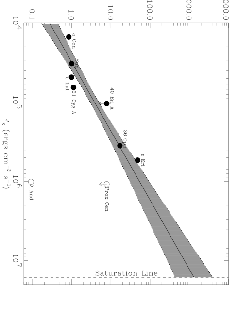
Figure 7: Measured mass loss rates (per unit surface area) plotted versus X-ray surface flux. A power law has been fitted to the solar-like GK dwarfs (filled circles), and the shaded region is the estimated uncertainty in the fit. Proxima Cen (M5.5 Ve) and $\lambda$ And (G8 IV-III+M V) appear to be inconsistent with this relation. The saturation line represents the maximum F_X value observed from solar-like stars.

The winds of cool main sequence stars have their origins in the coronae of these stars, so it is natural to wonder whether mass loss rates are correlated with coronal properties. The coronal X-ray luminosity is a good indicator of the magnetic activity level of a star and of the amount of material that has been heated to high coronal temperatures. Table 1 lists X-ray luminosities obtained with the ROSAT PSPC instrument, assuming Hipparcos stellar distances. Before comparing the mass loss rates with the X-ray emission, it is necessary to make the comparison equitable by dividing the mass loss measurements and X-ray luminosities by the stellar surface areas (see Table 1). Figure 7 shows mass loss rates per unit surface area plotted versus X-ray surface flux. For the solar-like GK dwarfs, the data suggest that more active stars have higher mass loss rates. However, the M dwarf Proxima Cen and the RS CVn system $\lambda$ And (G8 IV-III+M V) are inconsistent with this mass-loss/activity relation.

It has been argued previously that the strong flares on active M dwarfs should induce large mass loss rates, which could have a large impact on the Galactic ISM due to the large numbers of these stars (Mullan & Linsky, 1999). But the Proxima Cen data point in Figure 7 suggests that active M dwarfs instead have lower mass loss rates than the solar-like stars predict. This may be telling us something important about the wind acceleration process. Why does it not work as well on the M dwarfs? Is it due to the higher surface gravity, the generally higher coronal temperatures, stronger magnetic fields, or something else? Giampapa et al. (1996) present evidence that M dwarfs have a somewhat different magnetic field configuration than higher mass dwarfs, which could also be a factor. Addressing these issues will be an important challenge for future models of the wind acceleration mechanisms for coronal stars. However, there is only one M dwarf represented in Figure 7, and its mass loss rate is only an upper limit, so additional observations of M dwarfs are required to see whether Proxima Cen’s low mass loss rate is representative of all active M dwarfs.

The $\lambda$ And data point in Figure 7 is even more discrepant from the solar-like stars than Proxima Cen. The $\lambda$ And system is classified as an RS CVn binary. Such systems typically have high rotation rates forced by tidal locking between the two stars, which in turn leads to very high activity levels. The $\lambda$ And system certainly has the high activity, but is unusual in having both a long rotation period of 54 days and a long orbital period of about 21 days (Jetsu, 1996), with the difference between the two meaning that the two stars are not tidally locked. The $\lambda$ And primary, which surely dominates the X-ray flux and wind from the system, has a surface area about 55 times that of the Sun. The estimated mass loss rate of $5~{}\dot{M}_{\odot}$ is therefore surprisingly low, raising many of the same questions asked above regarding Proxima Cen. However, the uncertainty regarding the reality of the astrospheric absorption precludes any detailed consideration of its mass loss behavior at this time (see §2.1).

We fit a power law to the solar-like GK dwarfs in Figure 7, using a Monte Carlo technique to estimate the best fit and its uncertainty. In order to estimate the uncertainty in the fit, we have to estimate uncertainties for our mass loss rates. Unfortunately, the mass loss uncertainties depend entirely on systematic errors that are not easy to quantify. We now review some of these.

We must assume in our modeling that the ambient LISM is the same for our target stars, an assumption which is a potential source of error. However, as mentioned in §2.2, the requirements of pressure equilibrium suggest that LISM parameters should not vary too severely among our stars. Furthermore, Izmodenov et al. (2002) have found surprisingly little variability in heliospheric H I absorption in their models when different LISM parameters are assumed. Uncertainties in V_ISM and $\theta$ for each star will result in uncertainties in the mass loss rate measurements (see §2.2), but for these nearby stars we believe the uncertainties in these quantities should not be severe.

We must assume that the astrospheric absorption that we see is characteristic not only of the stellar mass loss along the line of sight, but also characteristic for the star as a whole. Solar wind properties depend somewhat on ecliptic latitude, at least during solar minimum conditions, so this is a potential source of error. However, the solar wind ram pressure variation with ecliptic latitude is not extreme (only about a factor of 1.5), so three-dimensional models of the heliosphere that take these variations into account do not suggest dramatic latitude-dependent variations in heliospheric structure (e.g., Pauls & Zank, 1997), so we do not think this is a big problem.

Perhaps the greatest potential source of uncertainty is the assumption that the stellar wind velocities are all close to $V_{w}=400$ km s^-1. We have no way of knowing how accurate this assumption might be, but we note that the size of an astrosphere and the amount of astrospheric absorption should scale roughly as the square root of the wind ram pressure, $P_{w}$ (Wood & Linsky, 1998). Since $P_{w}\propto\dot{M}V_{w}$, our mass loss estimates will to first order vary inversely with the assumed wind speed. Thus, if one believes that the wind velocity of a particular star could be a factor of 2 different from 400 km s^-1 (and solar wind variations span a range of about a factor of 2), our mass loss estimate for that star could be off by a factor of 2. Note that we could avoid this issue to a large extent if we chose to measure and discuss wind ram pressures rather than mass loss rates. Regardless of what wind velocity we choose to assume, the mass loss rate that we derive should be such that the wind ram pressure is the same, since it is the ram pressure rather than the wind velocity or mass loss rate alone that establishes the amount of astrospheric absorption (as mentioned above). However, the mass loss rate is the quantity that is of most astrophysical interest, so that is what we choose to discuss, even though this quantity cannot be measured as precisely as $P_{w}$ due to the additional necessary $V_{w}=400$ km s^-1 assumption.

Finally, uncertainties in the intrinsic Ly$\alpha$ profiles lead to uncertainties in the assessment of what model best fits the data (see §2.2 and Fig. 3). Unlike the previously listed systematic errors, at least in this case experimentation with the data provides us with some idea of the magnitude of this uncertainty. Considering all the possible sources of error listed above, we estimate uncertainties for the mass loss measurements to be factors of 2 (i.e., $\pm 0.3$ dex). These uncertainties are no better than educated guesses, but we note that the assumed factor of 2 errors are roughly consistent with the scatter of the GK star data points in Figure 7 about the best fit relation. If the systematic errors are really larger, one would expect to see more scatter, but a larger sample of stars is necessary to address this issue.

We also assume factor of 2 uncertainties for the X-ray luminosities, not because of measurement errors but because of potential variability. This assumption is consistent with the analysis of Ayres (1997), who estimated that the ROSAT PSPC fluxes for solar-like stars should cover a mininum-maximum range of about a factor of 4 during activity cycles like that of the Sun. We note that X-ray luminosities measured from the Einstein IPC instrument (Maggio et al., 1987; Schmitt et al., 1990) agree with the PSPC luminosities in Table 1 to within a factor of 2 in all cases.

The data points for the solar-like stars in Figure 7 are randomly varied within the assumed error bars mentioned above for both the mass loss rate and X-ray values, and a power law fit is performed for each trial. The line shown in Figure 7 is the average fit and the shaded region represents the 1 $\sigma$ uncertainty in the fit. In the figure, the relation is extended up to the saturation line, which indicates the maximum X-ray flux observed from solar-like stars (Güdel, Guinan, & Skinner, 1997). The assumption is that when coronal activity is at a maximum, coronal mass loss will be at a maximum as well. Quantitatively, the relation in Figure 7 is

$$\dot{M}\propto F_{x}^{1.15\pm 0.20}.$$ (1)

3.2 Mass Loss as a Function of Age

As stars age, their rotation rates ($V_{rot}$) slow down due to magnetic braking. As rotation slows, less magnetic activity is generated by the stellar dynamo, so X-ray fluxes decrease. There are a vast number of observational studies that have been directed toward measuring the relations between rotation and age (e.g., Skumanich, 1972; Soderblom et al., 1993) and X-ray flux and rotation (e.g., Pallavicini et al., 1981; Walter, 1982, 1983; Caillault & Helfand, 1985; Micela et al., 1985; Fleming et al., 1989; Stauffer et al., 1994). Quantitatively, Ayres (1997) estimates for solar-like stars:

$$V_{rot}\propto t^{-0.6\pm 0.1}$$ (2)

and

$$F_{x}\propto V_{rot}^{2.9\pm 0.3}.$$ (3)

Combining equations (1)–(3), we can obtain the following relation for mass loss and stellar age:

$$\dot{M}\propto t^{-2.00\pm 0.52}.$$ (4)

This is the first empirically derived relation describing the mass loss evolution of cool main sequence stars like the Sun. The relation suggests that mass loss decreases with time for solar-like stars.

Note that the real relations between $V_{rot}$, $F_{x}$, and $t$ are probably not simple power laws. Many of the references cited above have assumed more complicated functional forms that might be more physically realistic. Nevertheless, we choose simple power law representations from Ayres (1997) for the sake of convenience, since our derived relation between $\dot{M}$ and $F_{x}$ in equation (1) is a simple power law. (Our small sample size does not warrant the assumption of a functional form more complicated than a power law.) If we were to choose different relations from the literature, the quantitative form of equation (4) would change. However, all relations should yield the same qualitative result that mass loss decreases with time. For example, if we assume

$$F_{x}\propto\exp\left[\left(-2.20\pm 0.22\right)t^{0.5}\right]$$ (5)

from Walter & Barry (1991), then we compute

$$\dot{M}\propto\exp\left[\left(-2.53\pm 0.51\right)t^{0.5}\right],$$ (6)

where $t$ in equations (5) and (6) must be in Gyr units. Equation (6) appears very different from equation (4), but the differences are not actually severe. Equation (4) suggests that the solar mass loss rate was $30-330$ times larger when the Sun was 1/10 its present age, while equation (6) suggests that the solar wind was $20-90$ times larger at that time. There are differences between these two ranges, but the disagreement is not excessive considering the uncertainties.

The sample of stars that Ayres (1997) uses to derive relations (2) and (3) has a range of age and activity similar to our sample in Table 1, so combining equations (1)-(3) to obtain equation (4) is appropriate. It should be noted, however, that equation (2) clearly does not work well for very young stars ($t<0.3$ Gyr). Stars in young clusters tend to show broad distributions of rotation rates, meaning that the connection between age and rotation is not very strong for such stars (Simon, 1990; Soderblom et al., 1993). Thus, the predictions that equations (4) and (6) make for the mass loss rates of very young stars should be considered questionable.

A theoretical point that should be made regarding equations (1)-(3) is that while the connections between $V_{rot}$, $t$, and $F_{x}$ in (2)-(3) are rather direct, the physical connection between $\dot{M}$ and $F_{x}$ suggested by equation (1) must be indirect, because the X-ray flux presumably originates in closed field regions while the stellar wind arises in open field regions. The apparent correlation between $\dot{M}$ and $F_{x}$ in Figure 7 may mean that the underlying cause of stronger closed field regions that yield higher $F_{x}$ (i.e., the dynamo) also yields stronger open fields that accelerate more wind.

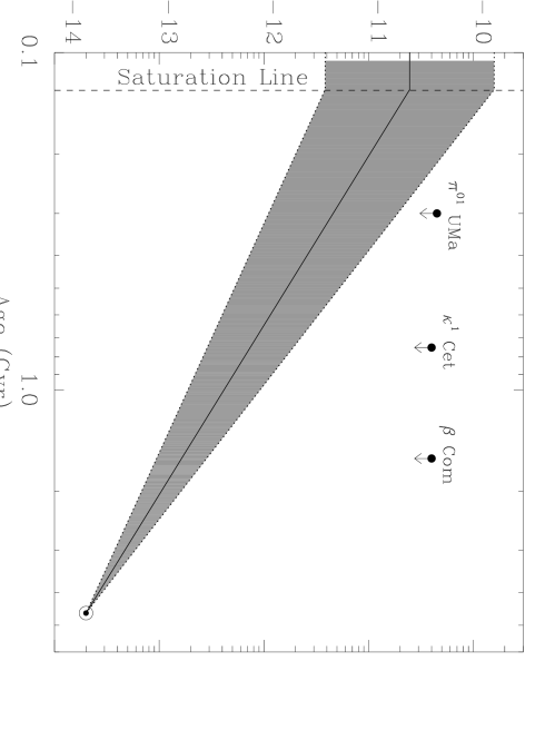
Figure 8: The mass loss history of the Sun suggested by the power law relation from Fig. 7. The upper limits are based on radio nondetections of three solar-like stars (Gaidos et al. 2000).

Figure 8 shows what relation (4) implies for the mass loss history of the Sun, once again assuming that the mass loss “saturates” when the coronal X-ray flux saturates. The solar wind may have been $\sim 1000$ times stronger when the Sun was very young, although we note once again that predictions for very early times are suspect. The upper limits in Figure 8 are based on nondetections of radio emission from three solar-like stars (Gaidos, Güdel, & Blake, 2000), illustrating that the high mass loss rates predicted for young stars are still consistent with our inability to detect radio emission from these stars. Note that the dependence of mass loss on time derived empirically in relation (4) likely results from a number of physical processes, including the evolution of magnetic fields in both strength and structure (i.e., the relative importance of closed vs. open structure).

Equation (4) has important ramifications for our understanding of the angular momentum evolution of cool stars, because it is the interaction between the stellar wind material and the magnetic field of the rotating star that is believed to provide the braking mechanism for stellar rotation on the main sequence, which is ultimately why rotation and activity both decrease with time. Higher mass loss rates can be expected to yield stronger braking. Models for how magnetic braking should affect stellar rotation suggest relations of the form

$$\frac{\dot{\Omega}}{\Omega}\propto\frac{\dot{M}}{M}\left(\frac{R_{A}}{R}\right)^{m},$$ (7)

where $\Omega$ is the angular rotation rate and $R_{A}$ is the Alfvén radius (Weber & Davis, 1967; Stepień, 1988; Gaidos et al., 2000). The exponent $m$ is a number between 0 and 2, where $m=2$ corresponds to a purely radial magnetic field. Mestel (1984) argues that more reasonable magnetic geometries suggest $m=0-1$.

We are interested in the time dependence of the quantities in equation (7). Equation (2) shows that $\Omega\propto V_{rot}\propto t^{-0.6}$, so $\dot{\Omega}\propto t^{-1.6}$ and $\dot{\Omega}/\Omega\propto t^{-1}$. We assume that neither the stellar mass ($M$) or radius ($R$) are time variable (see §3.3), while equation (4) indicates the time dependence of $\dot{M}$. The Alfvén radius is

$$R_{A}=\sqrt{\frac{V_{w}\dot{M}}{B_{r}^{2}}},$$ (8)

where $V_{w}$ is the stellar wind speed and $B_{r}$ is the radial magnetic field. Note that since equation (7) is computed assuming a simple, global magnetic field geometry, $B_{r}$ should be considered a disk-averaged field when relating it to the far more complex fields that stars like the Sun actually have. We assume that $V_{w}$ does not vary, which was also an assumption used in the derivation of mass loss rates from the astrospheric absorption (see §2.2). We can then express $B_{r}$ as a power law of time, $B_{r}\propto t^{\alpha}$, where from equations (4), (7), and (8) we find

$$\alpha=1/m-\left(1.00\pm 0.26\right)\left(m+2\right)/m.$$ (9)

Assuming that $m$ is in the physically allowable range of $m=0-2$ yields the upper limit $\alpha<-1.0$, while the more likely range of $m=0-1$ suggested by Mestel (1984) implies $\alpha<-1.2$. In any case, this result suggests that disk-averaged stellar magnetic fields decrease at least inversely with age for solar-like stars.

3.3 Relevance for Planetary Atmospheres

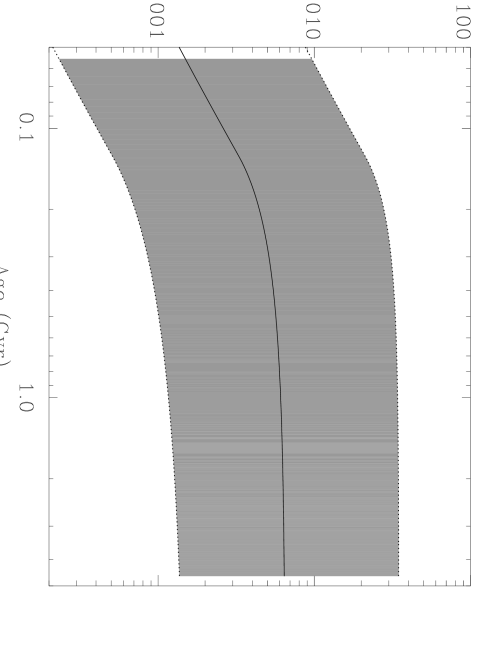
Figure 9: Cumulative mass loss for the Sun as a function of time, based on the mass loss history of the solar wind in Fig. 8.

Figure 9 shows the cumulative mass loss for the Sun as a function of time based on the relation in Figure 8. Despite the high mass loss rates predicted for the young Sun, the total mass that has been lost by the solar wind is still $\lesssim 0.03$ M_⊙, not enough to have dramatically altered the solar luminosity. Thus, the higher mass loss rates predicted for the young Sun are still not high enough to resolve the so-called “faint young Sun” paradox, which arises from standard evolutionary models of the Sun that predict that it should have been about 25% fainter 3.8 Gyr ago (Gough, 1981). The faintness of the young Sun appears to be inconsistent with the apparent existence of running water at these times on the surfaces of both Earth and Mars, which implies that planetary temperatures were not correspondingly lower (Sagan & Mullen, 1972; Kasting & Grinspoon, 1991).

If the solar mass loss rate was high enough in the past to decrease the Sun’s mass by $\sim 10$%, then the higher mass of the young Sun could increase the predicted solar luminosity enough that it no longer is a “faint young Sun” (Guzik, Willson, & Brunish, 1987). Although our analysis does suggest higher mass loss rates in the past, they are not high enough to change the solar mass sufficiently to resolve the faint young Sun paradox, and Figure 9 shows that almost all of the predicted mass loss occurs too early to be relevant to the issue anyway. A more likely resolution of the faint young Sun problem lies in atmospheric greenhouse effects that could allow Earth and Mars to maintain warm temperatures even with a fainter Sun (Walker, 1985; Kasting & Ackerman, 1986; Kasting & Grinspoon, 1991).

However, a more massive young solar wind may still have had profound effects on planetary atmospheres in our solar system. Exposure to the solar wind can erode planetary atmospheres, and the higher mass loss rates suggested for the young Sun in Figure 8 would exacerbate these effects. Solar wind sputtering processes have been proposed as having important effects for the atmospheres of both Venus and Titan (Chassefière, 1997; Lammer et al., 2000), but the Martian atmosphere may be the most interesting case of solar wind erosion, since the history of the Martian atmosphere is linked with the issue of whether water, and perhaps life, once existed on the surface.

Unlike Earth, the Martian atmosphere is not currently protected from the solar wind by a strong magnetosphere. There is evidence that Mars once had a magnetic field, which disappeared at least 3.9 Gyr ago (Acuña et al., 1999). At this point, the Martian atmosphere would have been exposed to a solar wind about 40 times stronger than the current wind according to Figure 8, which could have had a dramatic effect on the atmosphere. Mars appears to have had running water on its surface in the distant past, and there is evidence from isotopic ratios in the Martian atmosphere that Mars once had a thicker atmosphere that could have allowed a climate much more conducive to the existence of surface water (e.g., Carr, 1996; Jakosky & Phillips, 2001). However, today the Martian atmosphere is very thin, making stable surface water impossible, leading to the question of what happened to the thicker atmosphere and surface water. Solar wind erosion is a leading candidate for the cause of this change (Luhmann, Johnson, & Zhang, 1992; Perez de Tejada, 1992; Jakosky et al., 1994; Kass & Yung, 1995; Lundin, 2001), and if the young solar wind was stronger than today this possibility is even more likely.

4 SUMMARY

The interaction of a solar-like wind with the local ISM produces a population of hot hydrogen gas that is detectable in high resolution HST Ly$\alpha$ spectra of nearby stars. The amount of astrospheric H I absorption is a diagnostic for the mass loss rate of the wind. We have used mass loss rates measured from astrospheric absorption to study the dependence of mass loss on stellar age and activity. Our results are as follows:

1.

We present new mass loss measurements for four stars with previously detected astrospheric absorption, using hydrodynamic models of the astrospheres to assist in inferring mass loss rates from the absorption. The analyzed stars are $\epsilon$ Eri ($\dot{M}=30~{}\dot{M}_{\odot}$), 61 Cyg A ($\dot{M}=0.5~{}\dot{M}_{\odot}$), 36 Oph AB ($\dot{M}=15~{}\dot{M}_{\odot}$), and 40 Eri A ($\dot{M}<5~{}\dot{M}_{\odot}$).

2.

The astrospheres vary greatly in size depending on the stellar mass loss rate and the interstellar wind velocity seen by the star. The astrosphere of 61 Cyg A has an upwind bow shock distance of only 30 AU. In contrast, the upwind bow shock distance for $\epsilon$ Eri is about 1600 AU, with an apparent angular width of about $42^{\prime}$ as seen from Earth, making $\epsilon$ Eri’s astrosphere larger than the size of the full Moon.

3.

Combining our mass loss measurements with previous measurements, we study how the mass loss rates of cool main sequence stars depend on activity. The solar-like GK dwarfs show a correlation between mass loss rate (per unit surface area) and X-ray surface flux that can be described as a power law: $\dot{M}\propto F_{x}^{1.15\pm 0.20}$.

4.

Both Proxima Cen (M5.5 Ve) and the RS CVn system $\lambda$ And (G8 IV-III+M V) have mass loss rates significantly lower than would be predicted by the mass-loss/activity relation defined by the solar-like GK dwarfs, although we note that the astrospheric detection for $\lambda$ And must be considered uncertain.

5.

We combine our power law relation for mass loss and activity with rotation/activity and age/rotation relations from Ayres (1997) to derive a mass-loss/age relation for solar-like stars: $\dot{M}\propto t^{-2.00\pm 0.52}$. This relation suggests that the solar wind may have been as much as 1000 times stronger in the distant past.

6.

Our results are consistent with theoretical descriptions of the magnetic braking process that slows stellar rotation only if disk-averaged stellar magnetic fields decline at least inversely with time (i.e., $B\propto t^{\alpha}$, where $\alpha<-1$).

7.

Our suggestion that the young solar wind may have been significantly more massive than it is now could have important ramifications for the history of planetary atmospheres in our solar system. The more massive young solar wind suggested by our analysis is still not massive enough to resolve the so-called “faint young Sun” paradox, but the stronger wind does make it more likely that erosion by the solar wind has dramatically changed the properties of planetary atmospheres, with the Martian atmosphere being a particularly interesting case.

Table 1: Mass Loss Measurements

Star	Spectral	$d$	Surf. Area	Log Lx	$V_{ISM}$	$\theta$	$\log{\rm N(H~{}I)}$	$\dot{M}$	Refs.
	Type	(pc)	(A⊙)		(km s-1)	(deg)		($\dot{M}_{\odot}$)
$\alpha$ Cen	G2 V+K0 V	1.3	2.37	27.34	25	79	15.24	2	1,2,3
Prox Cen	M5.5 V	1.3	0.026	27.23	25	79	…	$<0.2$	3
$\epsilon$ Eri	K1 V	3.2	0.62	28.32	27	76	15.82	30	4,10
61 Cyg A	K5 V	3.5	0.45	27.26	86	46	14.11	0.5	5,10
$\epsilon$ Ind	K5 V	3.6	0.50	27.18	68	64	14.25	0.5	6,7,8
40 Eri A	K1 V	5.0	0.64	27.61	127	59	…	$<5$	5,10
36 Oph	K1 V+K1 V	5.5	0.88	28.28	40	134	16.10	15	9,10
$\lambda$ And	G8 IV-III+M V	26	55	30.53	53	89	15.20	5	6,7,8

References. — (1) Linsky & Wood 1996. (2) Gayley et al. 1997. (3) Wood et al. 2001. (4) Dring et al. 1997. (5) Wood & Linsky 1998. (6) Wood et al. 1996. (7) Müller et al. 2001a. (8) Müller et al. 2001b. (9) Wood et al. 2000a. (10) This paper.

Figure 6: (a) HST Ly$\alpha$ spectrum of 40 Eri A, showing broad H I absorption at 1215.8 Å and narrow D I absorption at 1215.4 Å. The upper solid line is the assumed intrinsic stellar emission line, and the dotted line shows the Ly$\alpha$ profile after only ISM absorption. The excess H I absorption on the blue side of the line is astrospheric absorption. The dashed and dot-dashed lines are predicted astrospheric absorption from astrospheric models with mass loss rates of $\dot{M}=1~{}\dot{M}_{\odot}$ and $\dot{M}=5~{}\dot{M}_{\odot}$, respectively. (b) Similar to (a), but with a different assumed stellar Ly$\alpha$ profile. The $\dot{M}=1~{}\dot{M}_{\odot}$ model (dashed line) now fits the data much better.

References

- Acuña et al. (1999) Acuña, M. J., et al. 1999, Science, 284, 790
- Ayres (1997) Ayres, T. R. 1997, J. Geophys. Res., 102, 1641
- Baranov, Izmodenov, & Malama (1998) Baranov, V. B., Izmodenov, V. V., & Malama, Y. G. 1998, J. Geophys. Res., 103, 9575
- Baranov & Malama (1993) Baranov, V. B., & Malama, Y. G. 1993, J. Geophys. Res., 98, 15157
- Baranov & Malama (1995) Baranov, V. B., & Malama, Y. G. 1995, J. Geophys. Res., 100, 14755
- Barnes, Evans, & Moffett (1978) Barnes, T. G., Evans, D. S., & Moffett, T. J. 1978, MNRAS, 183, 285
- Biermann (1957) Biermann, L. 1957, Observatory, 107, 109
- Caillault & Helfand (1985) Caillault, J. -P. & Helfand, D. J. 1985, ApJ, 289, 279
- Carr (1996) Carr, M. H. 1996, Water on Mars (New York: Oxford Univ. Press)
- Chassefière (1997) Chassefière, E. 1997, Icarus, 126, 229
- Dring et al. (1997) Dring, A. R., Linsky, J., Murthy, J., Henry, R. C., Moos, W., Vidal-Madjar, A., Audouze, J., & Landsman, W. 1997, ApJ, 488, 760
- Feldman et al. (1977) Feldman, W. C., Asbridge, J. R., Bame, S. J., & Gosling, J. T. 1977, in The Solar Output and its Variation, ed. O. R. White (Boulder: Colorado Associated University Press), 351
- Fleming, Gioia, & Maccacaro (1989) Fleming, T. A., Gioia, I. M., & Maccacaro, T. 1989, ApJ, 340, 1011
- Frisch (1993) Frisch, P. C. 1993, ApJ, 407, 198
- Gaidos, Güdel, & Blake (2000) Gaidos, E. J., Güdel, M., & Blake, G. A. 2000, Geophys. Res. Lett., 27, 501
- Gayley et al. (1997) Gayley, K. G., Zank, G. P., Pauls, H. L., Frisch, P. C., & Welty, D. E. 1997, ApJ, 487, 259
- Giampapa et al. (1996) Giampapa, M. S, Rosner, R., Kashyap, V., Fleming, T. A., Schmitt, J. H. M. M., & Bookbinder, J. A. 1996, ApJ, 463, 707
- Gough (1981) Gough, D. O. 1981, Solar Physics, 74, 21
- Güdel, Guinan, & Skinner (1997) Güdel, M., Guinan, E. F., & Skinner, S. L. 1997, ApJ, 483, 947
- Guzik, Willson, & Brunish (1987) Guzik, J. A., Willson, L. A., & Brunish, W. M. 1987, ApJ, 319, 957
- Hirshfeld & Ochsenbein (1985) Hirshfeld, A., & Ochsenbein, R. 1985, Sky Catalogue 2000.0, Vol. 2 (Cambridge: Cambridge University Press)
- Hünsch et al. (1999) Hünsch, M., Schmitt, J. H. M. M., Sterzik, M. F., & Voges, W. 1999, A&AS, 135, 319
- Irwin, Yang, & Walker (1996) Irwin, A. W., Yang, S. L. S., & Walker, G. A. H. 1996, PASP, 108, 580
- Izmodenov, Lallement, & Malama (1999) Izmodenov, V. V., Lallement, R., & Malama, Y. G. 1999, A&A, 342, L13
- Izmodenov, Lallement, & Wood (2002) Izmodenov, V. V., Lallement, R., & Wood, B. E. 2002, J. Geophys. Res., submitted
- Jakosky et al. (1994) Jakosky, B. M., Pepin, R. O., Johnson, R. E., & Fox, J. L. 1994, Icarus, 111, 271
- Jakosky & Phillips (2001) Jakosky, B. M., & Phillips, R. J. 2001, Nature, 412, 237
- Jetsu (1996) Jetsu, L. 1996, A&A, 314, 153
- Kamper (1976) Kamper, K. W. 1976, PASP, 88, 444
- Kass & Yung (1995) Kass, D. M., & Yung, Y. L. 1995, Science, 268, 697
- Kasting & Ackerman (1986) Kasting, J. G., & Ackerman, T. P. 1986, Science, 234, 1383
- Kasting & Grinspoon (1991) Kasting, J. F., & Grinspoon, D. H. 1991, in The Sun in Time, ed. C. P. Sonett, M. S. Giampapa, & M. S. Matthews (Tucson: The University of Arizona Press), 447
- Lallement & Bertin (1992) Lallement, R., & Bertin, P. 1992, A&A, 266, 479
- Lallement et al. (1995) Lallement, R., Ferlet, R., Lagrange, A. M., Lemoine, M., & Vidal-Madjar, A. 1995, A&A, 304, 461
- Lammer et al. (2000) Lammer, H., Stumptner, W., Molina-Cuberos, G. J., Bauer, S. J., & Owen, T. 2000, Planet. Space Sci., 48, 529
- Lemoine et al. (2002) Lemoine, M. L., et al. 2002, ApJS, in press
- Linsky & Wood (1996) Linsky, J. L., & Wood, B. E. 1996, ApJ, 463, 254
- Luhmann, Johnson, & Zhang (1992) Luhmann, J. G., Johnson, R. E., & Zhang, M. H. G. 1992, Geophys. Res. Lett., 19, 2151
- Lundin (2001) Lundin, R. 2001, Science, 291, 1909
- Maggio et al. (1987) Maggio, A., et al. 1987, ApJ, 315, 687
- McComas et al. (2001) McComas, D. J., Goldstein, R., Gosling, J. T., & Skoug, R. M. 2001, Space Sci. Rev., 97, 99
- Mestel (1984) Mestel, L. 1984, in Cool Stars, Stellar Systems, and the Sun, Third Workshop, ed. S. L. Baliunas & L. Hartmann (Berlin: Springer), 49
- Micela et al. (1985) Micela, G., Sciortino, S., Serio, S., Vaiana, G. S., Bookbinder, J., Golub, L., Harnden, F. R., Jr., & Rosner, R. 1985, ApJ, 292, 172
- Mullan & Linsky (1999) Mullan, D. J., & Linsky, J. L. 1999, ApJ, 511, 502
- Müller, Zank, & Lipatov (2000) Müller, H. -R., Zank, G. P., & Lipatov, A. S. 2000, J. Geophys. Res., 105, 27419
- Müller, Zank, & Wood (2001a) Müller, H. -R., Zank, G. P., & Wood, B. E. 2001a, ApJ, 551, 495
- Müller, Zank, & Wood (2001b) Müller, H. -R., Zank, G. P., & Wood, B. E. 2001b, in The Outer Heliosphere: The Next Frontiers, ed. K. Scherer et al. (Amsterdam: Pergamon), 53
- Nordgren et al. (1999) Nordgren, T. E., et al. 1999, AJ, 118, 3032
- Ortolani et al. (1997) Ortolani, A., Maggio, A., Pallavicini, R., Sciortino, S., Drake, J. J., & Drake, S. A. 1997, A&A, 325, 664
- Pallavicini et al. (1981) Pallavicini, R., Golub, L., Rosner, R., Vaiana, G. S., Ayres, T., & Linsky, J. L. 1981, ApJ, 248, 279
- Panagi & Mathioudakis (1993) Panagi, P. M., & Mathioudakis, M. 1993, A&AS, 100 343
- Parker (1960) Parker, E. N. 1960, ApJ, 132, 821
- Pauls & Zank (1997) Pauls, H. L., & Zank, G. P. 1997, J. Geophys. Res., 102, 19779
- Pauls, Zank, & Williams (1995) Pauls, H. L., Zank, G. P., & Williams, L. L. 1995, J. Geophys. Res., 100, 21595
- Perez de Tejada (1992) Perez de Tejada, H. 1992, JGR, 97, 3159
- Perryman et al. (1997) Perryman, M. A. C., et al. 1997, A&A, 323, L49
- Sagan & Mullen (1972) Sagan, C., & Mullen, G. 1972, Science, 177, 52
- Schmitt et al. (1990) Schmitt, J. H. M. M., Collura, A., Sciortino, S., Vaiana, G. S., Harnden, F. R., Jr., & Rosner, R. 1990, ApJ, 365, 704
- Schmitt, Fleming, & Giampapa (1995) Schmitt, J. H. M. M., Fleming, T. A., & Giampapa, M. S. 1995, ApJ, 450, 392
- Simon (1990) Simon, T. ApJ, 1990, 359, L51
- Skumanich (1972) Skumanich, A. 1972, ApJ, 171, 565
- Soderblom et al. (1993) Soderblom, D. R., Stauffer, J. R., MacGregor, K. B., & Jones, B. F. 1993, ApJ, 409, 624
- Stauffer et al. (1994) Stauffer, J. R., Caillault, J. -P., Gagné, M., Prosser, C. F., & Hartmann, L. W. 1994, ApJS, 91, 625
- Stepień (1988) Stepień, K. 1988, ApJ, 335, 907
- Vidal-Madjar et al. (1998) Vidal-Madjar, A., et al. 1998, A&A, 338, 694
- Walker (1985) Walker, J. C. G. 1985, Origins of Life, 16, 117
- Walter (1982) Walter, F. M. 1982, ApJ, 253, 745
- Walter (1983) Walter, F. M. 1983, ApJ, 274, 794
- Walter & Barry (1991) Walter, F. M., & Barry, D. C. 1991, in The Sun in Time, ed. C. P. Sonnett, M. S. Giampapa, & M. S. Matthews (Tucson: Univ. of Arizona Press), 633
- Weber & Davis (1967) Weber, E. J., & Davis, L., Jr. 1967, ApJ, 148, 217
- Wood, Alexander, & Linsky (1996) Wood, B. E., Alexander, W. R., & Linsky, J. L. 1996, ApJ, 470, 1157
- Wood & Linsky (1998) Wood, B. E., & Linsky, J. L. 1998, ApJ, 492, 788
- Wood et al. (2001) Wood, B. E., Linsky, J. L., Müller, H. -R., & Zank, G. P. 2001, ApJ, 547, L49
- Wood, Linsky, & Zank (2000a) Wood, B. E., Linsky, J. L., & Zank, G. P. 2000a, ApJ, 537, 304
- Wood, Müller, & Zank (2000b) Wood, B. E., Müller, H. -R., & Zank, G. P. 2000b, ApJ, 542, 493
- Wood et al. (2002) Wood, B. E., Müller, H. -R., Zank, G. P., & Linsky, J. L. 2002, in Cool Stars, Stellar Systems, and the Sun, Twelfth Workshop, in press
- Zank (1999) Zank, G. P. 1999, Space Sci. Rev., 89, 413
- Zank et al. (1996) Zank, G. P., Pauls, H. L., Williams, L. L., & Hall, D. T. 1996, J. Geophys. Res., 101, 21639