Chandra LETGS Observation of the Active Binary Algol

A high-resolution spectrum obtained with the low-energy transmission grating onboard the Chandra observatory is presented and analyzed. Our analysis indicates very hot plasma with temperatures up to $T\approx 15-20$ MK from the continuum and from ratios of hydrogen-like and helium-like ions of Si, Mg, and Ne. In addition lower temperature material is present since O vii and N vi are detected. Two methods for density diagnostics are applied. The He-like triplets from N vii to Si xiii are used and densities around $10^{11}$ cm^-3 are found for the low temperature ions. Taking the UV radiation field from the B star companion into account, we find that the low-Z ions can be affected by the radiation field quite strongly, such that densities of $3\times 10^{10}$ cm^-3 are also possible, but only assuming that the emitting plasma is immersed in the radiation field. For the high temperature He-like ions only low density limits are found. Using ratios of Fe xxi lines produced at similar temperatures are sensitive to lower densities but again yield only low density limits. We thus conclude that the hot plasma has densities below $10^{12}$ cm^-3. Assuming a constant pressure corona we show that the characteristic loop sizes must be small compared to the stellar radius and that filling factors below 0.1 are unlikely.

1 Introduction

Stellar coronae cannot be spatially resolved, yet they are thought to be highly structured just like the solar corona, whose X-ray emission comes almost exclusively from hot plasma confined in magnetic loops. So far the only way to infer structural information in such unresolved stellar point sources has been via eclipse studies in suitably chosen binary systems. Observations of the X-ray light curve can yield information on the location of the X-ray emission (Preś et al. 1995), although the eclipse mapping reconstruction problem is highly under-determined; after all, one is trying to reconstruct a three-dimensional intensity distribution from a one-dimensional light curve. Among a variety of problems discussed in detail by Schmitt (1998), a specific difficulty arises from the fact that in most eclipsing systems both components are known or likely to be X-ray emitters. Obviously the reconstruction problem is easier to solve in those cases where one of the binary components is X-ray dark. At X-ray wavelengths only two such systems have been studied so far, the eclipsing binary systems $\alpha$ CrB (cf. Schmitt & Kürster 1993) and $\beta$ Per (= Algol; Oord & Mewe 1989).

The Algol system actually consists of three components, a close eclipsing binary (containing a B8 main sequence star and a K2IV subgiant) and a more distant F-type star, which is not of interest for our purposes. The stellar parameters of the two stars of the eclipsing binary system (inclination angle is i=81^∘) are listed in Tab. 1. Algol is one of the brightest coronal X-ray emitters in the soft X-ray band and has been observed with essentially all X-ray satellites flown so far. Particular interest in Algol’s X-ray emission arises from the fact that no magnetic dynamos and magnetic activity phenomena should occur on stars of spectral type B8, since such stars are fully radiative and thus the primary component of Algol should be X-ray dark. In consequence, all of Algol’s X-ray emission is believed to originate from the cool secondary, which is rapidly rotating because it is tidally locked with the primary on the orbital time scale (2.8 days). We note in passing, however, that there is – in contrast to the totally eclipsing system $\alpha$ CrB (cf. Schmitt & Kürster 1993) – no observational proof for this assumption. Nevertheless, X-ray eclipses at secondary optical minimum are expected, yet not all observations of Algol at secondary minimum yield evidence for such eclipses. For example, a long observation of Algol with the EXOSAT satellite (White et al. 1986) centered on secondary optical minimum showed no indication for any eclipse, suggesting the interpretation of a corona with a scale height of more than a stellar radius or a somewhat peculiar configuration of the corona at the time of observation. On the other hand, a long ROSAT PSPC observation (Ottmann & Schmitt 1996) did show evidence for a partial eclipse of the quiescent X-ray emission, demonstrating that a significant fraction of the quiescent X-ray emission is emitted within a stellar radius. A BeppoSAX observation (Schmitt & Favata 1999, Favata & Schmitt 1999) of Algol showed the total eclipse of a long-duration flare, and a sequence of four ASCA observations of Algol at secondary eclipse showed evidence for both eclipses and absence of eclipses at different occasions.

Another method to provide information on structure in spatially unresolved data consists of spectroscopic measurements of density. If the density measurements are combined with the measurement of the volume emission measure EM, an estimate of the emitting plasma volume can be obtained; in an eclipsing binary these volumes will be subject to additional light curve constraints. With the high-resolution spectrometers onboard Chandra it is possible to carry out high-resolution X-ray spectroscopy for a wide range of coronal X-ray sources. We have obtained a Chandra high-resolution X-ray spectrum of Algol, which allows us to combine the information derived from X-ray light curves and X-ray spectroscopy. We will specifically discuss the Algol spectra obtained with the Low Energy Transmission Grating Spectrometer (LETGS).

Table 1: Properties of Algol A and B: mass $M$, radius $R$, effective temperature $T_{\rm eff}$, log g and spectral type are taken from Richards (1993) and references therein.

	Algol A	Algol B
d/pc	28
$M/M_{\odot}$	$3.7\pm 0.3$	$0.81\pm 0.05$
$R/R_{\odot}$	$2.9\pm 0.04$	$3.5\pm 0.1$
$T_{\rm eff}$/K	$13000\pm 500$	$4500\pm 300$
log g	$4.08$	$3.2$
Spectr. type	B8V	K2IV

2 Instrument description and Observation

The LETGS is a diffraction grating spectrometer covering the wavelength range between 5 – 175 Å (0.07 – 2.5 keV) with a resolution $\lambda/\Delta\lambda\sim 2000$ at the long wavelength end of the band pass; typical instrumental line widths are of the order 0.06 Å (FWHM) (cf., Ness et al. 2001a). A detailed description of the LETGS instrument is presented by Predehl et al. (1997). We note in passing that the LETGS uses a microchannel plate detector (HRC-S) placed behind the transmission grating without any significant intrinsic energy resolution. Thus in contrast to CCD based detectors the energy information for individual counting events is solely contained in the events’ spatial location.
Accounting for the instrumental line widths the symmetry of the grating is sufficient to co-add both sides of the spectrum in order to obtain a better SN ratio (Ness et al. 2001a). The thus obtained spectrum is shown in Fig. 1. A rich line spectrum with lines from Fe, Si, Ne, O, and N can be recognized between 6 and 30 Å as well as many Fe lines above 90 Å. Strong continuum emission is also apparent almost over the whole observed band pass; we note in passing that the spectrum shown in Fig. 1 has not been corrected for effective areas.

Figure 1: Top: LETGS spectrum of Algol in the range 1-40 Å. Clearly visible is the strong continuum and many prominent emission lines from Ne, Si, Fe, Mg, O, and N. The Ly_α lines from Mg xii (8.42Å), Ne x (12.14Å), O viii (18.97Å) and N vi (24.78Å) can be recognized.
Bottom: Wavelength range from 90-135 Å. Visible are the lines from Fe xviii at 94 Å  from Fe xxi at 117.5 Å and 128.7 Å, and from Fe xxiii/Fe xx at 133Å.

3 X-ray fluxes and light curve

Algol was observed with the above described instrumental setup between March, 12, 2000, 18:36 and March, 13, 2000, 17:13. The total on-time was 81.41 ksec, almost identical to the actual exposure time. During this time 106181 source counts were collected on the negative side and 101469 counts on the positive side. The high spectral resolution of the LETGS allows the computation of incident photon and energy fluxes without the need of any plasma emission model. In particular, since the LETGS wavelength range covers both the ROSAT and the Einstein wavelength ranges we can directly calculate fluxes corresponding to the respective band passes of these instruments without the need of any model. Using only bins with $A_{\rm eff}>0.1$ cm² and the distance d from Tab. 1 we compute a total X-ray luminosity of $1.4\,10^{31}$ erg/s. Restricting the wavelength range to the nominal ROSAT wavelength range (6.2-124 Å), we find $1.1\,10^{31}$ erg/s, within the Einstein band pass we find $1.0\,10^{31}$ erg/s (2.8-62 Å). These numbers can be compared with earlier measurements with these instruments. Berghöfer et al. (1996) report an X-ray flux of L${}_{X}=0.7\,10^{31}$ erg/s measured with ROSAT. This agrees with our Chandra measurement to within 30% so that significant long term variability can be excluded. Ottmann & Schmitt (1996) report an X-ray luminosity of L${}_{X}=20\,10^{31}$ erg/s during a flare, while their quiescent emission is consistent with the values reported by Berghöfer et al. (1996). Our measurement is therefore well within the range of luminosities found in earlier observations.
In order to compute the ephemeris of Algol, we used the expression $JD_{prim}$ = 2445739.003 + 2.8673285 $\times$ E (Kim 1989; E being an integer) for the times of primary minimum. Our Chandra observation covers the phases 0.74 to 1.06, i.e., outside optical secondary minimum. In Fig. 2 we show the background-subtracted X-ray light curve of the LETGS data (in the ranges 10 - 120 Å, 10 - 20 Å, 20 - 80 Å, and 80 - 120 Å). As is clear from Fig. 2, the light curve shows a more or less continuous decrease in intensity throughout the Chandra observations by a factor of 1.38 (10 - 120 Å), 1.22 (10 - 20 Å), 1.47 (20 - 80 Å), and 1.77 (80 - 120 Å). Phasing of the data suggests the existence of a primary minimum in X-rays, when the late-type star is located in front of the early-type star, but from our discussion above this appears highly unlikely. Since the Algol system is known to be able to produce giant flares, a far more plausible interpretation would be to interpret the X-ray light curve as the “tail” of a long-duration flare, possibly similar to the one observed by Schmitt & Favata (1999) with BeppoSAX. From this assumption, however, we would expect the radiation to become softer in time and to detect a cooling of the plasma. From Fig. 2 no evidence for softening can be deduced, rather the radiation becomes even harder. From the temperature dependent line ratios of the resonance lines of the H-like and He-like ions plotted in Fig. 3 again no evidence for cooling is apparent; the plasma might even become hotter with time, but at a very small rate. For oxygen the ratio raises from 3.6 $\pm$ 0.27 to 4.2 $\pm$ 0.35, for nitrogen from 2.7 $\pm$ 0.25 to 3.3 $\pm$ 0.37 and for magnesium from 1.7 $\pm$ 0.12 to 2.0 $\pm$ 0.16. Thus we find no indication for the ”tail” of a long duration flare from this spectral analysis. Other plausible scenarios can be thought of as, e.g., the time-evolution of one or more of the coronal active regions or rotational modulation.

Figure 2: Light curve of Algol in a hard, medium and a soft energy band.

Figure 3: Light curve of Algol in three different energy bands (top) and development of the temperature dependent ratios of Ly_α/He-like resonance line for Oxygen, Nitrogen and Magnesium.

4 Data analysis

The data extraction from the HRC-S and analysis of the spectra presented in this paper are identical to the methods described by Ness et al. (2001a). Specifically the spectra are extracted along the spectral trace without any pulse height correction scheme, the background is taken from nearby adjacent regions on the microchannel plate. The two dispersion directions are co-added, but the individual dispersed spectra can still be used to check for inconsistencies in the co-added spectrum. The thus obtained spectrum is shown in Fig. 1.

4.1 Analysis of the continuum

The total spectrum in Fig. 1 shows two components, a multitude of emission lines and a significant continuum. The shape of the continuum suggests thermal bremsstrahlung emission as the dominant continuum emission process. This assumption is supported by the high temperatures measured for Si, Mg, and Fe (cf. Tab. 4). We therefore use the formula

$$\frac{dW}{dV\ dt\ d\lambda} = 2.051\times 10^{-19}n_{e}^{2}T^{-1/2}\frac{G(\lambda,T)}{\lambda^{2}}e^{-143.9/(T\lambda)}$$ (1)

[erg cm^-3 s^-1 Å^-1]

(Mewe et al. 1986) for the specific volume emissivity $\frac{dW}{dV\ dt\ d\lambda}$ to model the continuum. $T$ is the plasma temperature in K and $c$ the speed of light in cm/s. The Gaunt factor $G(\lambda,T)=G_{\rm ff}(\lambda,T)+G_{\rm bf}(\lambda,T)$ is modeled as the sum of the free-free Gaunt factor

$$\log\,G_{\rm ff}(\lambda,T) = 0.355\lambda^{-0.06}\log\lambda$$

$$+0.3\lambda^{-0.066}\log\,\left(\frac{T}{10^{8}}\right)+0.0043$$

(Mewe et al. 1986) and the bound-free Gaunt factor

$$G_{\rm bf}(\lambda,T)=aT^{b}e^{cT^{d}}$$ (3)

with the parameters $a$, $b$, $c$, and $d$ adopted from Mewe et al. (1986). Introducing the variable $x=1/\lambda$ we derive from Eq. 1 an expression for the total number $dW$ of recorded photons divided by effective areas in each wavelength bin:

$$dW=B*G(\lambda,143.9/\alpha)/\sqrt{143.9/\alpha}*x^{2}e^{-\alpha x}$$ (4)

with $B=2.05\times 10^{-19}EM/(4\pi d^{2})*\Delta t*\Delta\lambda$, $\alpha=143.9/T$, and $x=1/\lambda$. The plasma temperature can be derived from $\alpha$ and the emission measure $EM=n^{2}V$ from $B$ while $\Delta\lambda$=0.01 Å (the binsize of the spectrum), and the exposure time $\Delta t$=81.41 ksec. Best fit parameters $B$ and $\alpha$ are obtained with a $\chi^{2}$ fit. In order to minimize the effects from the emission lines, we actually use the inverse spectrum to be compared with $1/dW(B,\alpha)$. In each iteration step we calculate the temperature from $\alpha$ with $T(\alpha)=143.9/\alpha$ and the Gaunt factor in each wavelength bin from Eqns. 4.1 and 3. From our best fit results we find $T=20.7$ MK and $EM=67.5\times 10^{52}$ cm^-3. This temperature is high, we note, however, that the sensitivity to the temperature is quite different in the different wavelength ranges. In Fig. 4 three such wavelength ranges are shown for three different choices of temperature and the same emission measure $EM=68\times 10^{52}$ cm^-3. Because of the flatness of bremsstrahlung spectra the choice of the temperature is not important above 18 Å, but the position of the cutoff does depend sensitively on temperature. The number of emission lines between 13 and 16 Å is quite high leading to line blends; the best fit bremsstrahlung continuum is therefore low (cf., middle panel of Fig. 4). With the bottom panel we wish to show that the assumption of $T=14.4$ MK provides a realistic description for all wavelength ranges and in particular for the region near the thermal cutoff of the X-ray spectrum. In this case 79% of the X-ray luminosity $L_{X}$ belongs to the continuum, thus $L_{X,cont}=1.1\times 10^{31}$ erg/sec. As a cross check we calculate the emission measure from the total luminosity and a mean radiative power loss due to bremsstrahlung of $1.5\times 10^{-23}$ erg cm³/sec, and obtain $EM=93\times 10^{52}$ cm^-3. From this exercise we note that the continuum can well be modeled with a bremsstrahlung spectrum, and our Chandra data are consistent with an emission measure $EM=68\times 10^{52}$ cm^-3 and a (peak) temperature at 15 MK.

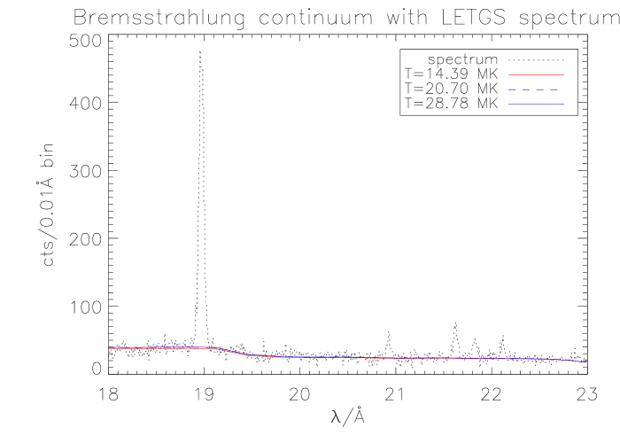
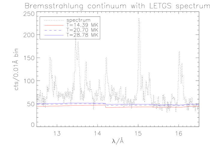
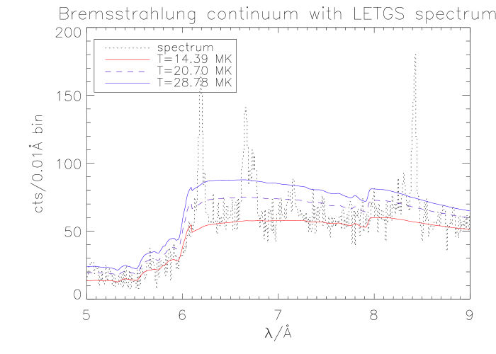
Figure 4: Modeled bremsstrahlung spectrum with $T=14$, 21, and 29 MK and $EM=68\times 10^{52}$ cm^-3 in comparison with the measured spectrum. The model is converted to LETGS counts by use of the effective areas from Pease et al. (Oct. 2000). Top: very little sensitivity to the temperature, middle: attempt to model overlaps with higher temperatures, bottom: strong dependence of temperature suggesting 15 MK the only temperature consistent with all wavelength ranges.

4.2 Extracted spectra and measured line ratios

Figure 5: (a,b) Spectrum (bold line) and best fit (thin solid line) for the triplets O vii (a) and N vi (b) for Algol. The dashed-dotted line represents the instrumental background.

Figure 6: (a,b) Same as Fig. 5 for Si xiii (a) and Mg xi (b). The unidentified line at 9.36 Å is also fitted with 57 cts.

For the analysis of emission lines we use a maximum likelihood method which compares the sum of a model and the instrumental background with the non-subtracted count spectrum. In this way Poisson statistics can be explicitly taken into account. The model spectrum consists of one or more lines with a variable or fixed spacing and a source background, which is assumed to be constant over the region of interest (i.e., the spectral lines under individual consideration). This assumption is well justified since both the instrumental background is quite flat as well as the source background (bremsstrahlung spectrum) once multiplied with the effective areas. The method includes Poisson fluctuations both in the line and background counts. Our code assumes the line profile functions to be Gaussian, but other shapes can be easily implemented. In this paper we used the CORA program, version 1.2, for the analysis. It has been developed and described by Ness et al. (2001a), and can be downloaded from http://ibiblio.org/pub/Linux/science/astronomy/.

The analysis was performed on the basis of the count spectrum. The measured line counts are given in Tab. 3 and we list the best fits of the wavelengths $\lambda$, the Gaussian line-widths, the number of line photons, and the source background $sbg$ measured in counts/Å which is assumed constant within the individual parts of the spectrum under consideration. In the last column we list the effective areas (as provided by Pease et al. Oct. 2000) as used for calculating line ratios needed for further analysis from the measurements; all errors in Tab. 3 are 1$\sigma$ errors. The first part of Tab. 3 contains the He-like triplets Si xiii, Mg xi, Ne ix, O vii, and N vi in combination with their H-like lines Si xiv, Mg xii, Ne x, O viii, and N vii. Since the Ne triplet is severely blended, the contaminating lines are also listed in Tab. 3.
For the density diagnostics of the higher temperature regions, five Fe xxi lines are also listed in Tab. 3, together with the ratios of each line with respect to the Fe xxi 128.73 Å line. For an estimate of optical depth effects, two Fe xvii lines were also measured and further analysis is performed in Sect. 7.

4.2.1 Analysis of He-like line ratios

We first discuss the lower temperature He-like line systems from oxygen and nitrogen. In Fig. 5 (a,b) we show the region around the O vii triplet at 22 Å and the N vi triplet at 28 Å together with best fits of the resonance, intercombination, and forbidden lines. All three lines are clearly detected above the background, which is actually dominated by continuum radiation from Algol itself (cf., Fig. 1).

In Fig. 6 (a,b) we show the Mg xi and Si xiii triplets together with our best fits. Obviously, the relative spectral resolution of the LETGS becomes smaller with smaller wavelengths, and at short wavelengths the Chandra HETGS performs far better. Still, the lines are at least partially resolved and line parameters can be determined by fitting a line template to the data whose relative position is fixed. In this fashion the Si xiii triplet blend can be fitted and the determined value for the f/i ratio is consistent with the low density limit. The Mg xi triplet is more complicated. While the Mg xi r-line is clearly detected, there are no clear detections of the i and f-lines. In particular, the emission line feature(s) found at the expected position of the Mg xi f-line is unusually broad, yet we are not aware of other strong contaminating lines in that region as is suggested by the fit in Fig. 6 (b). The determined line fluxes and hence line ratios do of course depend on the adopted background levels, yet in no case do we find an f/i-ratio consistent with the low density limit. Since this is in conflict with both the Si xiii data as well as the Fe xxi data discussed below, we consider the “detections” of the Mg xi i and f lines shown in Fig. 6 (b) and reported in Tab. 3 as spurious.

4.2.2 Analysis of the Ne ix triplet

Figure 7: The Ne ix triplet with blending lines from Fe xix/xvii. The fit is constrained to (f+i)/r=0.8, i.e., granting a meaningfull G ratio, assuming log$T<6.7$ (5 MK) for the Ne triplet.

The analysis of the Ne ix triplet is notoriously difficult, because of severe blending of the intercombination line at 13.55 Å with an Fe xix line at 13.52 Å (cf., Fig. 7 and Tab. 3). The Ne ix resonance and the forbidden lines are clearly detected, while the intercombination line is “lost” in a large line blend longward of the resonance line. Our fits indicate 665 counts in the r-line, 385 counts in the f-line, and 736 counts in the i-line blend. The question is how many of those 736 counts are due to the Ne ix i-line rather than Fe xix. In the following we estimate that by, first, constraining the fit to G=(f+i)/r=0.8, and, second, by extrapolating line fluxes from other Fe xix lines.

The fit shown in Fig. 7 was performed enforcing the boundary condition of G=0.8. With this constraint a reasonable fit is obtained with 147 counts in the intercombination line and the remaining 589 counts in the Fe xix line. We now discuss whether this line count of 589 counts is consistent with extrapolations from other Fe xix lines using MEKAL (Mewe et al. 1995) for calculating flux ratios. For this purpose we selected four other Fe xix lines suitable for comparison, i.e., they are sufficiently isolated and/or sufficiently strong. These lines are located at 13.79 Å, 14.67 Å, 101.5 Å, and 108.5 Å, and our fit results are listed in Tab. 2; for comparison we use as reference line the Fe xix at 13.52 Å. The measured flux ratios can be used for comparison with theoretical line flux ratios taken from MEKAL (Mewe et al. 1995). From the temperature analysis in Sect. 5 and from Tab. 4 we assume a temperature of 10 MK for extrapolating flux ratios from the theoretical fluxes.

Table 2: Measured line flux ratios for Fe xix and Fe xvii lines used for consistency checks of the treatment of the Ne ix blend in Fig. 7. Values for effective areas $A_{\rm eff}$ are taken from In-Flight Calibration by Pease et al. (31. October 2000). The measured ratios are corrected for interstellar absorption with the values from Tab. 3. Theoretical flux ratios are obtained from MEKAL (Mewe et al. 1995) assuming log$T=7.0$ (10 MK, cf. Tab. 4).

$\lambda$/Å	A [cts]	A/$\lambda$/$A_{\rm eff}$		Flux ratio
		$\sim$[erg/cm2]	$\lambda$/13.52	meas.	theor.
Fe xix lines			13.79	0.24 $\pm$ 0.05	0.30
13.52	588.98	1.66 $\pm$ 0.11	14.67	$<$ 0.12	0.11
13.79	147.30	0.40 $\pm$ 0.07	101.5	0.07 $\pm$ 0.02	0.16
14.67	$<$ 80.	$<$ 0.20	108.5	0.19 $\pm$ 0.02	0.42
101.5	77.670	0.11 $\pm$ 0.02	$\lambda$/13.79
108.5	204.00	0.29 $\pm$ 0.02	13.52	4.09 $\pm$ 0.85	3.3
			14.67	$<$ 0.49	0.39
			101.5	0.3 $\pm$ 0.08	0.56
Fe xvii lines			108.5	0.80 $\pm$ 0.18	2.5
15.00	1042.7	2.56 $\pm$ 0.09	Ratio for Fe xvii $\lambda$/13.84
13.84	114.20	0.31 $\pm$ 0.07	15.00	8.16 $\pm$ 2.0	12.9

The measured Fe xix and Fe xvii ratios listed in Tab. 2 indicate that the measured flux ratios are systematically smaller than the theoretical ratios from MEKAL. This effect is more significant when using the Chianti data base. But the general trend is quite convincing indicating the Fe xix lines at 13.52 Å and 13.79 Å to be well modelled in Fig. 7 and in Tab. 3. Also the results for Fe xvii at 13.84 Å seem to be realistic.

Eventually a reduction of Fe xix at 13.52 Å would cure the difference between measured and theoretical ratios, leading to a higher value of the intercombination line. This would mean a higher G ratio (i.e., a lower temperature) and a lower f/i ratio (i.e., a higher density). But this reduction, in combination with a reduced Fe xix at 13.79 Å flux, would also require an enhancement of the Fe xvii line at 13.84 Å in order to retain the sum of the blend at 13.79Å/13.84 Å, and the ratio of this line with the very strong 15 Å line would become smaller, which is the opposite effect of what would be intended with the reduction. We therefore trust our results obtained from the constrained fit only fixing the G ratio to 0.8.

4.2.3 Analysis of Fe xxi line ratios

Figure 8: Fitting of Fe xxi Top: Fe xxi (102.22 Å) in combination with Fe xix (101.55 Å) and $6^{th}$ order of Fe xvii (17.054 Å) Bottom: Fe xxii (117.17 Å) and Fe xxi (117.505 Å)

The analysis of most of the Fe xxi lines was straightforward. For the Fe xxi line at 121.21 Å only an upper limit could be determined. Some difficulties were encountered for the Fe xxi 102.22 Å and the Fe xxi 117.505 Å lines. The Fe xxi line at 102.22 Å is partially blended with the 6^th order of Fe xvii at the original wavelength at 17.054 Å. The Fe xxi line at 117.505 Å is found to be very broad such that it is difficult to find the correct wavelength position. In the top panel of Fig. 8 our model with the isolated Fe xix line at 101.55 Å together with Fe xxi at 102.22 Å and the 6^th order of Fe xvii is shown. In the bottom panel of Fig. 8 the Fe xxi at 117.505 Å is shown in combination with the strong, isolated Fe xxii line at 117.17 Å. In both cases the isolated lines are used to determine the line shift of our measurement in comparison with the theoretical wavelengths. In that way the expected wavelength position for the weaker, or blended lines under consideration was used for the fit.

Table 3: Measured line counts for Algol with 1$\sigma$ errors. Values of the total effective areas $A_{\rm eff}$ are taken from In-Flight Calibration by Pease et al. (31. October 2000). The Transmissions from the ISM are based on N(H i) = 2.5$\times 10^{18}$, N(He i)/N(H i) = 0.09, N(He ii)/N(H i) = 0.01

	$\lambda$ [Å]	$\sigma$ [Å]	A [cts]	sbg	$R_{\rm obs}=$f/i	$G_{\rm obs}=\frac{\rm i+f}{\rm r}$	$A_{\rm eff}$
				[cts/Å]	$[R]^{(2)}$	$[G]^{(2)}$	[cm2]
He-like and H-like (cf. Sects. 5 and 6.1.3)
Si xiv	6.19 $\pm$ 0.0016	0.025 $\pm$ 0.002	658.32 $\pm$ 35.06	5119			36.22
Si xiii$r$	6.65 $\pm$ 0.004		480.7 $\pm$ 35.95				37.54
$i$	6.69 $\pm$ 0.014	0.022$\pm$ 0.003	86.4 $\pm$ 33.10	5300	3.64 $\pm$ 1.44	0.83 $\pm$ 0.15	37.38
$f$	6.74 $\pm$ 0.006		314.1 $\pm$ 30.60		[3.66 $\pm$ 1.45](2)	[0.84 $\pm$ 0.15](2)	37.16
Mg xii	8.42 $\pm$ 0.0016	0.02 $\pm$ 0.002	578.04 $\pm$ 33.13	5900			32.28
Mg xi$r$	9.17 $\pm$ 0.0015		224.12 $\pm$ 26.15				27.69
$i$	9.23 $\pm$ 0.0015	0.02 $\pm$ 0.002	84.85 $\pm$ 23.29	5400	0.90 $\pm$ 0.36	0.72 $\pm$ 0.22	27.42
$f$	9.31 $\pm$ 0.0015		76.09 $\pm$ 22.80		[0.90 $\pm$ 0.37](2)	[0.73 $\pm$ 0.23](2)	27.24
Ne x	12.14 $\pm$ 0.0004	0.021 $\pm$ 0.0008	2481.48 $\pm$ 56.31	6510			24.96
Ne ix	cf. Sect.4.2.2
$r$	13.46 $\pm$ 0.003	0.022 $\pm$ 0.0022	665.03 $\pm$ 37.21				26.16
$i$	13.56 $\pm$ 0.011	0.022 $\pm$ 0.0022	146.65 $\pm$ 31.74	6000	2.63 $\pm$ 0.61	0.80	26.23
$f$	13.71 $\pm$ 0.004	0.022 $\pm$ 0.0022	385.38 $\pm$ 30.83		[2.62 $\pm$ 0.61](2)	–	26.29
Fe xix	13.52 $\pm$ 0.003	0.022 $\pm$ 0.0022	588.98 $\pm$ 39.82		[fit constrained to G=0.8]		26.21
Fe xix	13.79 $\pm$ 0.007	0.022 $\pm$ 0.0022	147.29 $\pm$ 28.81				26.31
Fe xvii	13.84 $\pm$ 0.07	0.022 $\pm$ 0.0022	114.18 $\pm$ 27.80				26.32
O viii	18.9701 $\pm$ 0.0004	0.0262 $\pm$ 0.0004	2882.96 $\pm$ 57.81	3150			24.29
O vii$r$	21.62 $\pm$ 0.016	0.022 $\pm$ 0.002	262.49 $\pm$ 22.6				15.58
$i$	21.82 $\pm$ 0.021	0.021 $\pm$ 0.004	128.77 $\pm$ 18.7	2439	0.94 $\pm$ 0.2	0.95 $\pm$ 0.16	15.34
$f$	22.11 $\pm$ 0.022	0.020 $\pm$ 0.004	120.9 $\pm$ 18.0		[0.94 $\pm$ 0.2](2)	[0.97 $\pm$ 0.16](2)	15.32
N vii	24.8 $\pm$ 0.0012	0.03 $\pm$ 0.0012	1119.05 $\pm$ 38.38				15.23
N vi$r$	28.81 $\pm$ 0.007	0.037 $\pm$ 0.008	141.33 $\pm$ 21.10				13.57
$i$	29.11 $\pm$ 0.011	0.058 $\pm$ 0.012	188.23 $\pm$ 25.53	1700	0.20 $\pm$ 0.08	1.60 $\pm$ 0.37	13.57
$f$	29.55 $\pm$ 0.011	0.021 $\pm$ 0.007	37.5 $\pm$ 14.31		[0.21 $\pm$ 0.09](2)	[1.65 $\pm$ 0.38](2)	12.76
Fe xxi density diagnostics (cf. Sect. 6.2)					$\frac{\rm F(\lambda)}{\rm F(128.73\textrm{\tiny\AA})}^{(1)}$	ISM
	97.87	0.049	67.20 $\pm$ 14.50	334	0.12 $\pm$ 0.03	0.9206	7.17
	102.22	0.043	94.11 $\pm$ 16.1	350	0.18 $\pm$ 0.07	0.9111	6.64
	117.505	0.058	92.10 $\pm$ 16.00	225	0.20 $\pm$ 0.04	0.8734	6.13
	121.22	0.055	$<36$	117	$<0.09$	0.8633	5.55
	128.73	0.058	266.32 $\pm$ 20.90	73	1	0.8420	3.64
Ne ix consistency check (cf. Sect. 4.2.2)
Fe xix	14.66 $\pm$ 0.007	0.02 $\pm$ 0.002	$<$ 80	5010		0.999	26.99
Fe xix	101.63 $\pm$ 0.007	0.043 $\pm$ 0.006	77.67 $\pm$ 14.55	350		0.9124	6.69
Fe xix	108.45 $\pm$ 0.007	0.054 $\pm$ 0.006	203.53 $\pm$ 19.42	311		0.8964	6.42
Fe xvii optical thickness (cf. Sect. 7)					$\frac{\rm F(15.03\textrm{\tiny\AA})}{\rm F(15.27\textrm{\tiny\AA})}$	$\frac{\rm F(15.03\textrm{\tiny\AA})}{\rm F(15.27\textrm{\tiny\AA})}^{(2)}$
Fe xvii	15.026 $\pm$ 0.001	0.021 $\pm$ 0.001	1018.44 $\pm$ 38.93	4500			27.21
Fe xvii	15.27 $\pm$ 0.008	0.023 $\pm$ 0.003	364.71 $\pm$ 28.92	4500	2.79 $\pm$ 0.25	[2.81 $\pm$ 0.25](2)	27.42
Fe temperatures (cf. Sect. 5)					${\rm A[cts/cm^{2}]}^{(2)}$
Fe xvii	15.28 $\pm$ 0.004	0.024 $\pm$ 0.003	375.73 $\pm$ 29.30	4500	14.22 $\pm$ 1.11		26.42
Fe xviii	16.082 $\pm$ 0.0031	0.03 $\pm$ 0.004	572.78 $\pm$ 35.95	4500	21.07 $\pm$ 1.32		27.19
Fe xxii	117.25 $\pm$ 0.093	0.053 $\pm$ 0.06	483.14 $\pm$ 25.91	225	78.56 $\pm$ 4.21		6.15
Fe xx	118.81 $\pm$ 0.014	0.0623 $\pm$ 0.013	97.87 $\pm$ 16.98	225	16.26 $\pm$ 2.82		6.02
Fe xx	121.98 $\pm$ 0.009	0.0675 $\pm$ 0.009	180.88 $\pm$ 19.23	138	34.19 $\pm$ 3.64		5.29

⁽¹⁾ Fluxes accounting for $A_{\rm eff}$ and ISM as in last but one column. ⁽²⁾ Fluxes corrected for $A_{\rm eff}$ listed in the last column.

5 Temperature diagnostics

Table 4: Temperature diagnostics from the flux ratios of Ly_α/He_r for the ions Si xiv/xiii, Mg xii/xi, Ne x/ix, O viii/vii, and N vii/vi. $T_{\rm M}$ denotes the peak formation temperatures. Temperatures for various Fe ions are calculated in the same manner by using theoretical line ratios from MEKAL.

	Lyα/r	$T$(H-He)	$T_{\rm M}$
		[MK]	[MK]
$\frac{\rm Si\,\mathsc{xiv}}{\rm Si\,\mathsc{xiii}}$	1.54 $\pm$ 0.14	14.6 $\pm$ 0.5	15.85/10.0
$\frac{\rm Mg\,\mathsc{xii}}{\rm Mg\,\mathsc{xi}}$	2.41 $\pm$ 0.31	10.4 $\pm$ 0.5	10.0/6.3
$\frac{\rm Ne\,\mathsc{x}}{\rm Ne\,\mathsc{ix}}$	4.33 $\pm$ 0.26	7.5 $\pm$ 0.2	5.62/3.98
$\frac{\rm O\,\mathsc{viii}}{\rm O\,\mathsc{vii}}$	8.03 $\pm$ 0.71	4.8 $\pm$ 0.2	3.16/2.2
$\frac{\rm N\,\mathsc{vii}}{\rm N\,\mathsc{vi}}$	8.37 $\pm$ 1.28	3.4 $\pm$ 0.2	2.0/1.4
		flux ratio	$T$/MK
Fe xvii/Fe xviii
15.265/16.078		0.67 $\pm$ 0.07	7.93 $\pm$ 0.43
Fe xxi/Fe xxii
117.51/117.17		0.19 $\pm$ 0.03	10.41 $\pm$ 0.71
Fe xxi/Fe xxii
121.83/117.51		2.28 $\pm$ 0.46	10.38 $\pm$ 0.83
118.66/117.51		1.08 $\pm$ 0.27	10.73 $\pm$ 1.22

We carry out temperature diagnostics using temperature sensitive line ratios of Ly_α/He_r and of Fe y/Fe ${\mathsc{y}+1}$. The results are listed in Tab. 4. The ratios Ly_α/He_r were calculated from the line fluxes corrected for effective areas, as listed in Tab. 3. We assume plasma emissivities as calculated in the Codes MEKAL (Mewe et al. 1985; Mewe et al. 1995) and SPEX (Kaastra et al. 1996) and compare the measured ratios with the calculated emissivity ratios in order to derive line formation temperatures. The results are listed in Tab. 4 as $T$(H-He).

In addition we also investigate the temperature of Fe emitting layers with various Fe flux ratios (cf. Tab. 4 bottom). We used the photon fluxes corrected for effective areas from Tab. 3 and compared the ratios with theoretical ratios derived with MEKAL and SPEX, in the same manner as for the Ly_α/He_r ratios. The theoretical flux of the Fe xviii 16.078 Å was corrected (enhanced) by a factor of 2.14 following Mewe et al. (2001).
From this analysis we find a cooler component of 8 MK, which is consistent with the Ly_α/He_r result for Ne. We also find hotter plasma at 10.5 MK in which the highly ionized Fe ions are formed. The ratios and derived temperatures are listed in Tab. 4. Clearly, a multitude of spectral components is present in the X-ray spectrum and we defer a discussion of the admissible emission measure distributions to a forthcoming paper.

6 Density diagnostics

Estimates of coronal density can be obtained from the density sensitive f/i ratio of He-like triplets and from the Fe xxi line ratios. The He-like N vi, O vii, and Ne ix ions probe the lower temperature components, while the Mg xi, Si xiii, and the Fe xxi ions are used to probe the higher temperature components of the coronal plasma. The low-Z He-like ions are sensitive at densities log($n_{e}$) between 9 and 12, while the high-Z He-like ions can only be used for higher densities above log$(n_{e})>$12. Lower densities log$(n_{e})>11$ at high temperatures $\approx$ 10 MK can be diagnosed from the Fe xxi ratios.

6.1 He-like ions

Figure 9: He-like densities $n_{e}$ from the ions O vii, N vi, and Ne ix. For comparison the theoretical curve assuming $\phi/\phi_{c}=0$ is also plotted (cf. Eq. 5).

Figure 10: He-like densities $n_{e}$ from the Si xiii ion.

6.1.1 Theory of He-like triplets

The theory of the atomic physics of He-like triplets has been extensively described in the literature (Gabriel & Jordan 1969, Blumenthal et al. 1972, Mewe & Schrijver 1978, Pradhan et al. 1981, Pradhan & Shull 1981, Pradhan 1982, Pradhan 1985, and recently Porquet & Dubau 2000, Porquet et al. 2001, and Ness et al. 2001a).

In this paper we will determine electron densities $n_{e}$ from the equation

$$R(n_{e})\ =\frac{\rm f}{\rm i}\ =\ \frac{R_{0}}{1+\phi/\phi_{c}+n_{e}/N_{\rm c}}\,$$ (5)

where $R_{0}$ denotes the low density limit and the parameter $N_{\rm c}$ the so-called critical density (cf. Tab. 5), around which the observed line ratio is density-sensitive. Finally, the parameters $\phi$ (the radiative absorption rate from $2\,^{3}S$ to $2\,^{3}P$ induced by an external radiation field) and $\phi_{c}$ describe the additional possible influence of the stellar radiation field on the depopulation of the ${}^{3}S$ state (cf., Sect. 6.1.2). Values for $R_{0}$ and $N_{\rm c}$ used in this paper are listed in Tab. 5. Also listed are the peak formation temperatures $T_{\rm M}$ for the ions.

Table 5: Atomic Parameters for He-like triplets. $T_{\rm M}$ is the peak line formation temperature (MEKAL), $R_{0}$ is the low-density limit and $N_{\rm c}$ is the density were $R$ falls to half its low-density value. $R_{0}$ and $N_{\rm c}$ are taken from Pradhan & Shull (1981) and Blumenthal et al. (1972).

ion	$T_{\rm M}$/MK	$R_{0}$	$N_{\rm c}/(10^{10}$ cm${}^{-3})$
Si xiii	10.0	2.67	3900
Mg xi	6.3	2.6	620
Ne ix	4.0	3.5	59.0
O vii	2.2	3.95	3.40
N vi	1.4	6.0	0.53

6.1.2 Influence of the stellar radiation field

Given the effective temperature of 13000 K of Algol A and its close proximity to Algol B (cf., Tab. 1), we must check to what extent the X-ray radiation originating from the corona of Algol B is influenced by the UV radiation from Algol A; the UV-radiation from the Algol B component itself is small when comparing its effective temperature with Capella ($T_{\rm eff}\leq$5000 K) and the values computed for $\phi/\phi_{c}$ to be used in Eq. 5 as derived by Ness et al. (2001a). Also the measurements of other G and K type stars, as presented by Ness et al. (2001c) suggest Algol B not to contribute to the total radiation field. Following Ness et al. (2001a) we used IUE measurements of Algol in order to derive radiation temperatures for the desired wavelengths, listed in Tab. 6. From this we calculated values $\phi/\phi_{c}$ for N vi, O vii, and Ne ix using a dilution factor of

$$W=\frac{1}{2}\left[1-\left\{1-\left(\frac{r_{\star}}{a}\right)^{2}\right\}^{1/2}\right]=0.01$$ (6)

(Mewe & Schrijver 1978) using as distance between Algol A and B $a=14.6\,R_{\sun}$ (Forbes 1997) and the radius of Algol A $r_{\star}=3.5\,R_{\sun}$ (Tab. 1). The result of our analysis is listed in Tab. 6. Since we assumed the worst case scenario, we find the maximally possible values $\phi/\phi_{c}$, so that the effects are not negligible for O vii and not zero even for Ne ix. We do point out, however, that in the phases between 0.74 and 1.06 (cf. Sect. 3) much of the visible coronal emission could originate from regions not illuminated by the B star. With an inclination angle of $81.5^{\circ}$ and the assumption of a uniform distribution of the coronal plasma, geometrical considerations lead to the result that at phase $\phi=1$ only plasma near the polar regions can be illuminated by the primary component. A detailed discussion of these geometrical considerations is given in Ness et al. (2001b). In the following analysis we calculate coronal densities with and without the effects of the radiation field from the B star, i.e., assuming $\phi/\phi_{c}=0$ and with the values for $\phi/\phi_{c}$ from Tab. 6.

Table 6: Investigation of the influence of the stellar radiation field originating from the B8 star. Measured fluxes from the IUE satellite $F_{\lambda}$ are converted to intensity $I_{\lambda}$ taking into account limb darkening effects using $\epsilon=0.44$ for the U band (Díaz-Cordovés et al. 1995).

	N vi	O vii	Ne ix
$\lambda_{\rm f\rightarrow i}$/Å	1900	1630	1266
$I_{\rm pot}$/eV	552.1	739.3	1195.3
$\frac{F_{\lambda}}{(10^{-10}\frac{\rm ergs}{\rm cm^{2}\,s\,\textrm{\tiny\AA}})}$	$20\pm 2$	$22\pm 2.2$	$20\pm 6$
$\frac{I_{\lambda}}{(10^{7}\frac{\rm ergs}{\rm cm^{2}\,s\,\textrm{\tiny\AA}\,strd})}$	$9.1\pm 0.91$	$9.98\pm 1.0$	$9.1\pm 2.7$
$T_{\rm rad}$/K	$12066\pm 186$	$12708\pm 190$	$13686\pm 560$
dilution factor	0.01
$\phi/\phi_{c}$	24.74 $\pm$ 2.41	2.18 $\pm$ 0.29	0.1 $\pm$ 0.03

6.1.3 Densities with the He-like ions

The measured ratios f/i, corrected for $A_{\rm eff}$ (Pease et al. Oct. 2000; the values are listed in the last column of Tab. 3), as quoted in Tab. 3, were used for density diagnostics. The theoretical curves from Eq. 5, with the values $\phi/\phi_{c}$ from Tab. 6 and the other parameters from Tab. 5, are plotted in Figs. 9 and 10 for each ion in comparison with our measurements for f/i with 1$\sigma$ errors. For the low-Z elements O, N, and Ne we also considered the case of no radiation field from the B star affecting the emitting layers with a line-dotted line in Fig. 9. The influence is most severe for N vi and O vii, but is also visible for Ne ix. Assuming a negligible radiation field from the primary component we obtain definite deviations from the low density limit for N vi and O vii and a marginal deviation for Ne ix; in the latter the latter case the 2$\sigma$ error includes the low density case. In these cases we find densities between 1–2 $\times 10^{11}$ cm^-3 (cf., Tab. 7). Assuming the full radiation field supplied from the B star to be effective the sensitivity of our measurements to detect densities is significantly reduced because the difference between the R-value in the high density case (R = 0) and low-density case becomes smaller and smaller. Specifically, for our Algol LETGS spectrum we find that the data are consistent with the low-density limit for nitrogen and neon, and even for oxygen the low density limit is included within the 2$\sigma$ error bars. For silicon and magnesium radiation effects are unimportant. The derived f/i-ratio for silicon is consistent with the low density limit, while our measurements for magnesium (formally) yield densities of $\approx$ log n${}_{e}=13$; as discussed in Sect. 4.2.1 and Fig. 6 (b), we consider the measurements of the i and f lines in magnesium spurious.

6.2 Density diagnostic with Fe xxi

In addition to He-like ions, ions with more than two electrons can be used as a density diagnostic. The ground configuration of Fe xxi 1s²2s²2p² splits up into ${}^{3}P$, ${}^{1}D$, ${}^{1}S$. The energy difference between the ground state ${}^{3}P_{0}$ and the excited levels ${}^{3}P_{1}$ and ${}^{3}P_{2}$ is 9 eV and 14.5 eV, respectively, and 30 eV between ground state and ${}^{1}D_{2}$. In low-density plasmas virtually all atoms are in the ground state ${}^{3}P$, while in high-density plasmas a Boltzmann equilibrium with the higher level will be obtained. Consequently, from excited levels certain lines will appear only in high-density plasmas. In contrast to He-like lines the appearance of certain lines is an indicator of high-density plasmas.

Our measurements of four Fe xxi ratios, corrected for effective areas and interstellar absorption are listed in Tab. 3 (effective areas and values from interstellar absorption are listed in the last two columns) and plotted in comparison with theoretical flux ratio vs. $n_{e}$ curves obtained with Chianti (Dere et al. 2001) in Figs. 11 and 12. As can be seen from Figs. 11 and 12, only low density limits or upper limits are obtained for all Fe xxi line ratios. Similar results are obtained when using the ratios from Brickhouse et al. (1995). The most sensitive upper limit (log n${}_{e}<11.52$) comes from the Fe xxi 102.2 Å/128.7 Å ratio, and is a factor $\sim$ 24 below the upper limit derived for the Si xiii triplet, which is formed at similar temperatures. This comparison clearly shows that Fe xxi line ratios yield far more sensitive density constraints at high temperature as compared to He-like triplets from magnesium, silicon, and higher ions.

Figure 11: Density diagnostic with Fe xxi ions. 1$\sigma$ errors are indicated with dashed line style (used 2$\sigma$ error for 102 Å ratio).

Figure 12: Density diagnostic with Fe xxi ions.

7 Optical depth effects

The Chandra Algol spectrum contains a number of strong Fe xvii lines which are sensitive to optical depth effects. In order to estimate the optical depth, we use an ”escape factor” model with a homogeneous mixture of emitters and absorbers in a slab geometry (e.g., Kaastra & Mewe 1995, Mewe et al. 2001). In this geometry the escape factor is $P(\tau)\sim[1+0.43\tau]^{-1}$. Significant optical depths will lead to resonant scattering in strong lines.

If one considers two lines produced by the same ion, the ratio of the optical depths is given by

$$\frac{\tau_{1}}{\tau_{2}}=\frac{\lambda_{1}\ f_{1}}{\lambda_{2}\ f_{2}}.$$ (7)

Therefore, one must look for lines from the same ion and large difference in oscillator strength or wavelength. In the solar context one usually studies the ratio of the strong Fe xvii 15.03 Å resonance line ($f=2.66$) and another, nearby Fe xvii line with a small oscillator strength (e.g., 15.265 Å, $f=0.593$). Estimating the escape factor $P$ from $P=\left(\frac{15.03\leavevmode\nobreak\ {\mathrm{\AA}}}{15.27\leavevmode\nobreak\ {\mathrm{\AA}}}\right)_{\rm meas}/\left(\frac{15.03\leavevmode\nobreak\ {\mathrm{\AA}}}{15.27\leavevmode\nobreak\ {\mathrm{\AA}}}\right)_{\tau=0}$ we can deduce the optical depth.

For the measured Fe xvii 15.03/15.265 photon flux ratio we obtain a formal fit result of 2.81 $\pm$ 0.25 (cf. Tab. 3). This ratio does depend on the assumed background value and can vary between 2.32 and 3.45 when varying the source background (between 4000 and 5000 cts/Å; comp. Tab. 3). In this particular wavelength region (cf., Fig. 4, middle) line blending is severe and a correct “eye” placement of the continuum is difficult. However, our continuum modeling predicts relative stable values of 4500 cts/Å so that we are confident that our quoted result is correct and not affected by systematic errors from the placement of the continuum background. We point out that this measurement agrees remarkably well with the same line ratio as measured in Capella (Mewe et al. 2001); this is interesting because in Capella no measurements of density could be obtained.

The measured photon flux ratio must be compared to the $\tau=0$ flux ratio, which can be deduced either from theory or laboratory measurements. With SPEX we predict a ratio of 3.5, thus $P=(2.81\pm 0.25)/3.5=0.8\pm 0.07$, and therefore $\tau=0.57\pm 0.26$. With Chianti (Dere et al. 2001), a ratio of $\approx 4$ is expected for $\tau=0$, and using $P=(2.81\pm 0.25)/4=0.7\pm 0.06$ we find $\tau=0.98\pm 0.3$. In either case we find optical depths significantly different from zero (at $\sim 2-3\sigma$ level).

Unfortunately theory does not agree with experiment. The very same line ratio can be measured in the Livermore Electron Beam Ion Trap (EBIT; Brown et al. 2001, Laming et al. 2000). These experiments typically yield Fe xvii 15.03/15.265 photon flux ratios in the range 2.5 - 3.0, which are significantly different from those expected theoretically. Also, Brown et al. (2001) point out that contamination of the 15.265 Å with Fe xvi further lowers the observed 15.03/15.265 photon flux ratio. Comparing the Algol (and Capella) flux ratios in 15.03/15.265 to the values quoted by Brown et al. (2001) we therefore conclude that the observations are fully consistent with an optical thin plasma without any significant optical depth with possibly some contamination arising from Fe xvi. It is worrying that the theoretically predicted emission from some of the strongest emission lines observed in solar and stellar X-ray spectra appears to be wrong by $\approx$ 30 percent.

Table 7: Summary of derived densities.
^⋆ Resulting density values accounting for stellar radiation fields.
^⋆⋆ 2$\sigma$ upper limit.

He-like triplets
	f/i	log($n_{e}$)
Si xiii	3.66 $\pm$ 1.44	$<$12.9
Mg xi	0.90 $\pm$ 0.37	n.a.
Ne ix	2.62 $\pm$ 0.61	11.30 $\pm$ 0.60
⋆Ne ix		$<$11.57
O vii	0.94 $\pm$ 0.20	11.04 $\pm$ 0.13
⋆O vii		10.54 $\pm$ 0.53
N vi	0.21 $\pm$ 0.09	11.16 $\pm$ 0.23
⋆N vi		10.13 $\pm$ 0.93
Fe xxi ratios
$\lambda/$Å	ratio	log($n_{e}$)
97.87	0.12 $\pm$ 0.03	$<$12.19
102.22	0.18 $\pm$ 0.03	$<11.52^{\star\star}$
117.51	0.20 $\pm$ 0.04	$<$12.63
121.22	$<$0.09	$<$12.4

8 Discussion and Interpretation

From the derived parameters we can obtain structural information on Algol’s corona. From the lower temperature He-like ions definite coronal densities could be determined, from the higher temperature He-like ions as well as from the Fe xxi line ratios (cf., Tab. 7) upper limits to the coronal density at a temperature of 10 MK can be derived. Since EM = $n_{e}^{2}\,V$, typical coronal volumes $V$ can be estimated from the recorded emission measures.

We now assume that Algol’s corona is composed of a multitude of individual but identical loops, all of which obey the loop scaling equation (Rosner et al. 1978)

$$n_{e}\,L=1.3\times 10^{6}\,T_{\rm apex}^{\,2},$$ (8)

with the densities $n_{e}$, the apex temperature $T_{\rm apex}$, and the loop semilength $L$, all in $cgs$ units. Of course, the apex temperature $T_{\rm apex}$ cannot be directly measured, it must however be close to the formation temperature of the ion with the highest ionization temperature and it can certainly not exceed the temperature of the bremsstrahlung continuum (Sect. 4.1). It is also clear that in Algol one is most likely dealing with a distribution of X-ray emitting loops as is the case in the solar corona. However, our data does not allow us to constrain the parameters of these distributions and therefore we model the distributions by their presumed mean values. From Tab. 4 we conclude that the apex temperatures $T_{\rm apex}$ must be approximately 15 MK, which is also supported by the continuum temperature, while from Tab. 7 we conclude that log $n_{e}<$ 11.5. Obviously the densities at 15 MK could be arbitrarily low. However, if we assume that the material at 15 MK is in thermal pressure equilibrium with the material at 2 MK (where the O vii line is produced) we estimate densities in the range log $n_{e}$ $\sim$ 9.7 - 10.2, depending on whether the X-ray emitting corona of Algol B is immersed in the UV radiation field of Algol A or not. For log $n_{e}=$ 11.5 we compute $L=9\times 10^{8}$ cm while for densities log $n_{e}$ = 9.7 - 10.2 we find $L=180-460\times 10^{8}$ cm. In either case, the loop lengths are much smaller than the stellar radius of 2.45 $\times 10^{11}$ cm so that we assume to deal with an essentially planar geometry. If we assume “canonical loops” with circular cross sections of a tenth of the loop length, the volumes of such coronal building blocks are in the range 2.5 10²⁵ cm³ to 3 10³⁰ cm³, again depending on the assumed density, and in all cases one requires at least 1000 loops (or more) in order to account for the total observed emission measure.

Let us next assume that the considered loops are semicircular and extend to height

$$H=\frac{2L}{\pi}.$$ (9)

We define the coronal filling factor as the ratio between the available volume $4\pi R^{2}H$ and the actual volume of X-ray emitting material $V_{\rm cor}=EM/n_{e}^{2}$:

$$f=\frac{V_{\rm cor}}{V_{\rm available}}=\frac{EM}{8n_{e}^{2}R^{2}L},$$ (10)

where $R$ denotes the stellar radius. Inserting the scaling law to replace $L$ with $T_{\rm apex}$ and $n_{e}$, we finally find

$$f=9.6\times 10^{-8}\frac{EM}{n_{e}R^{2}T_{\rm apex}^{2}}=9.6\frac{EM_{52}}{n_{10}R_{11}^{2}T_{6}^{2}}$$ (11)

[$$EM_{52}=EM/10^{52}\,{\rm cm}^{-3},R_{11}=R/10^{11}\,{\rm cm},$$

$$T_{6}=T_{\rm apex}/10^{6} ,n_{10}=n_{e}/10^{10}\,{\rm cm}^{-3}$$ K].

Using the continuum values $EM_{52}=68$ and $T_{6}$ = 15 we find $f\times n_{e}=5\times 10^{9}$ cm^-3. Since the filling factor $f$ can be unity at most, we deduce that $n_{min}=5\times 10^{9}$ cm^-3 and the actual density ought to exceed that value. Interestingly, $n_{min}T_{\rm apex}/T_{\rm O\mathsc{vii}}$ is close to the density determined from demanding that the high temperature material is at the same pressure as the O vii emitting material (assuming that it is immersed in the primary’s radiation field). Alternatively, density values of $1.5\times 10^{10}$ cm^-3 lead to filling factors of $\approx$ 0.3. These densities can only be reached without the illuminating UV radiation field of the primary component. The overall phase range covered by the Chandra LETGS observations is 0.32. During that period the star rotates by 115^∘; therefore most of the hemisphere visible at the beginning of our observations are not visible at the end. The observed light curve (cf. Fig. 2) with its slowly decreasing trend does not appear to give the impression of coming from a number of unrelated regions, rather, it appears to come from the same region on the star. This is only possible if the region is located near the pole (in which case it would be immersed in the radiation field) or if it is fortuitously located in a equatorial region which happens to be visible during the whole phase interval. While the latter possibility cannot be excluded, the former option appears more plausible given the previous evidence for polar activity in Algol (Schmitt & Favata 1999), the available VLBI images of Algol (Mutel et al. 1998) and the general occurrence of polar spots in Doppler images in general. It is attractive to interpret the observed X-ray emission as arising from the circumpolar regions, possibly from a long-duration flare similar to the one observed by Schmitt & Favata (1999). Assuming as height the limit inferred from the eclipsing BeppoSAX flare (H $\leq$ 7 10¹⁰ cm) and as filling factor arbitrarily a value of 1 percent (which is the surface area of the circumpolar polar cap), we find a volume of $4\times 10^{32}$ cm³, which requires densities of $2.5\times 10^{10}$ cm^-3 when combined with the observed emission measures. These densities refer to the hot material at temperatures of $\approx 15$ MK. Clearly, these densities are fully consistent with the observed upper limits.

Figure 13: Temperatures required for asserting certain filling factors (cf. Eq. 12) assuming constant pressures calculated from the densities and temperatures measured for O vii. For the emission measure we use the value obtained from the continuum $EM=68\times 10^{52}$ cm^-3.

Continuing in our picture of “canonical” loops, we can compare a typical pressure scale height $H_{p}=5000\,T_{\rm apex}/(g/g_{\odot})=3.8\times 10^{11}$ cm using $T_{\rm apex}=15$ MK and $g/g_{\odot}=0.2$, with a typical loop size $L\approx 30\times 10^{8}$ cm (Eq. 8). Since $H_{p}>>L$, the assumption of constant pressure is well justified. Hence $P=n_{e}*T$ must be constant and thus Eq. 11 can be rewritten as

$$f=9.6\frac{EM_{52}}{P_{16}R_{11}^{2}T_{6}}\Longleftrightarrow T_{6}=9.6\frac{EM_{52}}{P_{16}R_{11}^{2}f}$$ (12)

[$$P_{16}=n_{e}*T/10^{16}$$ cm^-3 K],

which relates the unknown filling factor with the - in principle - measured parameters stellar radius, emission measure and coronal pressure. In Fig. 13 we plot the dependence of temperatures on filling factor for different pressures, using Eq. 12; the emission measure obtained from the continuum (Sect. 4.1) was used. The pressures are calculated from the measured temperatures (Tab. 4) and densities (Tab. 7) for O vii. In the case of the radiation field from the B star to influence the density diagnostics, a lower limit for the pressure of $P=8\times 10^{16}$ cm^-3 K, using the peak formation temperature $T=2.2$ MK is calculated, while we obtain $P=50\times 10^{16}$ cm^-3 K for the higher density from omitting the possible effects from the radiation field and the higher temperature obtained from the Ly${}_{\alpha}/$r ratio (Tab. 4).

It is clear that $T$ must exceed 10 MK and is very likely below 30 MK. For low pressure (P${}_{16}=8$) the filling factor would have to exceed 0.45, while for high pressure (P${}_{16}=50$) the filling factor would have to be in the interval $0.07<f<0.21$. Since we feel that filling factors $f\sim 1$ are unlikely, we favor a high pressure scenario.

9 Conclusions

The high-resolution spectrum obtained with the LETGS on board the Chandra observatory shows a large number of emission lines and an unusually strong continuum. We analyze both the emission lines and the continuum relying exclusively on ratios of individual lines. The LETGS observation interval covered the orbital phases between 0.74 to 1.06, the light curve appears to indicate a relative state of quiescence. A slow decline is seen, but cannot be attributed to the decay of a giant flare, since no cooling and no softening of the overall emission is detected. The total luminosity is $L_{X}=1.4\,10^{31}$ erg/sec, roughly consistent with the X-ray luminosities found previously with Einstein and ROSAT.

We analyzed the continuum in order to determine an upper temperature and an overall emission measure. The continuum can well be modeled with a bremsstrahlung continuum and a temperature of 15 MK can be derived which is consistent with the peak formation temperature of, e.g., Si xiv which is clearly detected. Optical depth effects leading to resonant line scattering were analyzed and ruled out. The ratio of Fe xvii lines at 15 Å and 15.27 Å are used for testing optical depth effects, but inconsistencies in the atomic line data were found. From our findings in comparison with other measurements with the LETGS we conclude that a line ratio of $\approx 2.8$ must occur in plasmas with $\tau=0$.

The measurement of plasma temperatures is carried out using line ratios of ions from the same element in adjacent ionization stages as, e.g., Ly_α and He-like resonance lines. At least two temperature components are found, allowing N vi (3.2 MK) and Si xiv (14.2 MK) to be formed. This is consistent with our findings for Fe xxi/Fe xxii ($\approx 10\,$MK).

For the density diagnostics with the He-like triplets the UV radiation field originating from the B star companion was analyzed. We found significant effects for the ions N vi, O vii, and even for Ne ix, however, the illumination geometry of the primary B-type star is unclear. We therefore considered both the case with full illumination and no illumination of the coronal plasma.The determined densities range around $10^{10}-10^{11}$ cm^-3, while for the ions Si xiii and Ne ixwe find only upper limits. This is also found for all Fe xxi line ratios,but these upper limits are consistent with densities $10^{10}-10^{11}$ cm^-3 as well.

A detailed analysis discussing structural information deduced from the derived temperatures and densities is presented. The assumptions used for this discussion are that Algol’s corona is composed of a multitude of individual but identical (semi circular canonical) loops, all of which obey the RTV loop scaling equation. We further assume that the material is in thermal pressure equilibrium at 15 MK. From these assumptions we conclude from our measurements that these loops have semi-lengths of $L=9\times 10^{8}$ cm. The assumption of the emitting plasma to be immersed in the external radiation field leads us to lower densities and thus loop lengths of up to $L=460\times 10^{8}$ cm, which is, however, still much smaller than the stellar radius. The emission measure derived from the analysis of the continuum in combination with the densities allows us to define constraints on the coronal filling factor. However, different pressures ranging between 8 and $50\times 10^{16}$ cm^-3 K are possible, depending on whether the emitting plasma is immersed in the external radiation field or not. A low pressure plasma (i.e., effects from the radiation field are severe) requires a large filling factor, while the high pressure scenario allows a lower filling factor.

References

- (1) Berghöfer T.W., Schmitt J.H.M.M., & Cassinelli J.P., 1996, A&A 118, 481
- (2) Blumenthal G.R., Drake G.W., & Tucker W.H., 1972, ApJ 172,205
- (3) Brickhouse N.S., Raymond J.C., and Smith B.W., 1995, ApJS 97, 551
- (4) Brown G.V., Beiersdorfer P., Liedahl D.A., et al., 1998, ApJ 502, 1015
- (5) Brown G.V., Beiersdorfer P., Chen H., et al., 2001, ApJ 557, L75
- (6) Díaz-Cordovés J., Claret A., & Giménez A., 1995, A&AS 110, 329
- (7) Dere K. P., Landi E., Young P. R., & Del Zanna G. 2001 ApJS 134, 331, The Chianti database, with extension to X-Ray wavelengths
- (8) Favata F. & Schmitt J.H.M.M., 1999, A&A 350, 900
- (9) Forbes T.G. in Magnetic Reconnection in the Solar Atmosphere (eds Bently, R.D. & Mariska, J.T.) Vol. 111, 259 (ASP Conf. Ser., 1997)
- (10) Gabriel A.H. & Jordan C., 1969, MNRAS 145, 241
- (11) Kaastra J.S., Mewe R., & Nieuwenhuijzen H., 1996, in UV and X-ray Spectroscopy
- (12) Kaastra J. & Mewe R., 1995, A&AL 302, L13
- (13) Kim Ho-Il, 1989, ApJ 342, 1061
- (14) Laming J.M., Kink I., Takacs E., et al., 2000, ApJ 545, L161
- (15) Mewe R., Gronenschild E.H.B.M., & van den Oord G.H.J., 1985, A&AS 62, 197
- (16) Mewe R., Kaastra J.S., & Liedahl D.A., 1995, Legacy 6, 16 (MEKAL)
- (17) Mewe R., Raassen A.J.J., Drake J.J., et al., 2001, A&A 368, 888
- (18) Mewe R. & Schrijver J., 1978, A&A 65, 99
- (19) Mewe R., Lemen J.R., & van den Oord G.H.J., 1986, A&AS 65, 511
- (20) Mutel R.L., Molnar L.A., Waltman E.B., & Ghigoi F.D., 1998, ApJ 507, 371
- (21) Ness J.U., Mewe R., Schmitt J.H.M.M., et al., 2001a, A&A 367, 282
- (22) Ness J.U., Mewe R., Schmitt J.H.M.M., et al., 2001b, PASP submitted (Poster at Stellar Coronae 2001)
- (23) Ness J.U., Mewe R., Schmitt J.H.M.M., et al., 2001c, PASP submitted (Talk at CS12)
- (24) Oord G.H.J. van den, Mewe R., 1989, A&A 213, 245
- (25) Ottmann R. & Schmitt J.H.M.M., 1996, A&A 307, 813
-
(26)
Pease D.O., Drake J.J., Johnson C.O., et al.
2000, SPIE 4012, 700
Effective areas for the LETGS
measured Oct 31, 2000, downloaded from
http://asc.harvard.edu/cal/Links/Letg/User/ - (27) Porquet D. & Dubau J., 2000, A&AS 143, 495
- (28) Porquet D., Mewe R., Dubau J., et al. 2001, A&A 376, 1113
- (29) Pradhan A.K., 1982, ApJ 263, 477
- (30) Pradhan A.K., 1985, ApJ 288, 824
- (31) Pradhan A.K., Norcross D.W., & Hummer D.G., 1981, ApJ 246,1031
- (32) Pradhan A.K. & Shull J.M., 1981, ApJ 249,821
- (33) Predehl P., Braeuninger H., Brinkman A., et al., 1997, Proc. SPIE 3113, 172
- (34) Preś P., Siarkowski M., & Sylwester J., 1995, MNRAS 275, 43
- (35) Richards M.T., 1993, ApJ 86, 255
- (36) Rosner R., Tucker W.H., & Vaiana G.S., 1978, ApJ 220, 643
- (37) Schmitt J.H.M.M. 1998, ASP Conference Series, Vol. 154
- (38) Schmitt J.H.M.M. & Favata F., 1999, Nature 401, 44
- (39) Schmitt J.H.M.M. & Kürster, 1993, Science 262, 215
- (40) White N.E., Culhane J. L., Parmar A. N., et al., 1986, ApJ 301, 262