M75, a Globular Cluster with a Trimodal Horizontal Branch.
I. Color-Magnitude Diagram

Abstract

Deep $UBVI$ photometry for a large field covering the distant globular cluster M75 (NGC 6864) is presented. We confirm a previous suggestion (Catelan et al. 1998a) that M75 possesses a bimodal horizontal branch (HB) bearing striking resemblance to the well-known case of NGC 1851. In addition, we detect a third, smaller grouping of stars on the M75 blue tail, separated from the bulk of the blue HB stars by a gap spanning about 0.5 mag in $V$. Such a group of stars may correspond to the upper part of a very extended, though thinly populated, blue tail. Thus M75 appears to have a trimodal HB. The presence of the “Grundahl jump” is verified using the broadband $U$ filter. We explore the color-magnitude diagram of M75 with the purpose of deriving the cluster’s fundamental parameters, and find a metallicity of ${\rm[Fe/H]}=-1.03\pm 0.17$ dex and $-1.24\pm 0.21$ in the Carretta & Gratton (1997) and Zinn & West (1984) scales, respectively. We discuss earlier suggestions that the cluster has an anomalously low ratio of bright red giants to HB stars. A differential age analysis with respect to NGC 1851 suggests that the two clusters are essentially coeval.

1 Introduction

Adequate interpretation of the color-magnitude diagrams (CMDs) of globular clusters (GCs) is important for many astrophysical and cosmological reasons. The horizontal branch (HB) evolutionary phase plays a particularly significant role in that regard. Because the observational properties of HB stars are extremely sensitive to the physical parameters of GCs, HB stars can impose invaluable constraints on the initial conditions that characterized the Galaxy in its infancy.

Metallicity, [Fe/H], is the “first parameter” influencing HB morphology: Metal-rich clusters have, in general, more red HB stars than blue HB stars and vice versa for the metal-poor GCs. The existence of GCs which have the same [Fe/H] but different HB morphologies indicates that one or more second parameters exists. Despite the fact that the problem has received much attention since it was first discovered (Sandage & Wildey 1967), the second parameter(s) responsible for the spread in HB types at a given [Fe/H] has (have) not been firmly established. Understanding the second parameter is arguably one of the most important tasks that must be accomplished before the age and formation history of the Galaxy can be reliably determined (e.g., Searle & Zinn 1978; van den Bergh 1993; Zinn 1993; Lee, Demarque, & Zinn 1994; Majewski 1994).

Much recent debate has focused on whether the predominant second parameter is age (e.g., Lee et al. 1994; Stetson, VandenBerg, & Bolte 1996; Sarajedini, Chaboyer, & Demarque 1997; Catelan 2000; Catelan, Ferraro, & Rood 2001b; Catelan et al. 2001a; VandenBerg 2000), but mass loss, helium and $\alpha$-element abundances, rotation, deep mixing, binary interactions, core concentration, and even planetary systems have been suggested as second parameters. It is likely that the second parameter phenomenon is in fact a combination of several individual quantities and phenomena related to the formation and chemodynamical evolution of each individual star cluster, implying that the several individual second-parameter candidates have to be “weighted” on a case-by-case basis (e.g., Fusi Pecci et al. 1993; Fusi Pecci & Bellazzini 1997; Rich et al. 1997; Sweigart 1997a, 1997b; Kraft et al. 1998; Sweigart & Catelan 1998; Soker 1998; Ferraro et al. 1999a; Catelan 2000; Soker & Harpaz 2000; Catelan et al. 2001a, 2001b). In this context, it has been extensively argued that an understanding of GCs presenting the second-parameter syndrome internally—i.e., those with bimodal HBs—is of paramount importance for understanding the nature of the second-parameter phenomenon as a whole (e.g., Rood et al. 1993; Stetson et al. 1996; Borissova et al. 1997; Catelan et al. 1998a; Fusi Pecci & Bellazzini 1997; Walker 1998).

Unfortunately, the current list of GCs known to have a bimodal HB is not large; probably only NGC 1851, NGC 2808 and NGC 6229 are universally recognized as “bona fide” bimodal-HB clusters, following the definition of the term provided by Catelan et al. (1998a). However, as discussed by Catelan et al., there are several other GCs whose poorly investigated CMDs, once improved on the basis of modern CCD photometry, may well move them into the “bimodal HB” category. Outstanding among those is M75 (NGC 6864).

M75 is a moderately metal-rich (${\rm[Fe/H]}\simeq-1.3$ in the Zinn & West 1984, hereafter ZW84, scale; Harris 1996), dense {$\log[\rho_{0}/(M_{\odot}{\rm pc}^{-3})]=4.9$; Pryor & Meylan 1993} and distant ($R_{\odot}\simeq 19$ kpc) halo GC located about 13 kpc from the Galactic center (Harris 1996). Since it is not affected by high reddening—$E(\bv)=0.16$ mag, according to the Harris catalogue—we find it somewhat surprising that the only CMD for this cluster available in the literature seems to be the photographic one provided by Harris (1975). This is even more puzzling in view of the fact that it has been over a quarter of a century since Harris called attention to some intriguing characteristics of this cluster’s CMD—such as an abnormally high ratio $R$ of HB to red giant branch (RGB) stars and the presence of an unusually strong blue HB component for such a moderately metal-rich cluster. Interest in the CMD of this particular cluster seems to have been revived only very recently, when Catelan et al. (1998a) pointed out that “new CCD investigations are especially encouraged [for M75], since the latest CMD available (Harris 1975) is strongly suggestive of an NGC 1851-like HB bimodality.” Note that, due to M75’s distance, the Harris photographic CMD was only barely able to reach the HB level of the cluster.

It is the main purpose of the present paper to present the first deep CCD photometry of M75, and to investigate whether—as suggested by Catelan et al. (1998a)—M75 can be classified as yet another bona fide bimodal-HB cluster. In §2, we discuss our observing runs and data reduction techniques. In §3, the cluster CMD is discussed in detail, revealing not only a clearly bimodal HB but also a third grouping of blue tail stars clearly separated from the bulk of the blue HB, and likely indicating the cooler end of a very extended, though thinly populated, blue tail. The presence and radial distribution of blue straggler stars (BSS) is also discussed, and Harris’s (1975) suggestion of an abnormally high $R$ ratio is addressed. In §4, we evaluate the “photometric metallicity” and reddening of the cluster, and in §5 we derive its age relative to NGC 1851.

In a companion paper (Corwin et al. 2001, hereinafter Paper II), we will present a detailed analysis of the variable star population in the cluster.

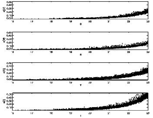
Figure 1: Formal errors of the NTT photometry from the daophot package as a function of the mean $U,B,V,I$ magnitudes for each star.

2 Observations and Data Reduction

Our analysis is based on the following observational material:

1. A set of “blue” $U,B$ and “red” $V,I$ CCD frames obtained in June 1997 on the ESO-NTT telescope with the $1024\times 1024$ and $2048\times 1900$ CCD cameras. The array scales were $0.361\arcsec\,{\rm pixel}^{-1}$ and $0.266\arcsec$ ${\rm pixel}^{-1}$, giving fields of view of about $6.16\arcmin\times 6.16\arcmin$ and $9.08\arcmin\times 8.42\arcmin$. The data consist of one short (60-20 sec) exposure image in $B,V,I$, and two long exposure images (900-300 sec) in $U,B,V,I$.

2. Fourteen $B,V$ frames obtained in July 1999 at the 0.9-meter telescope of the Cerro Tololo Inter-American Observatory with a $2048\times 2048$ CCD camera. The pixel scale of $0.396\arcsec\,{\rm pixel}^{-1}$ gave an observing area of $13.5\arcmin\times\ 13.5\arcmin$.

3. Ten $B,V$ frames obtained in July 1989 at the 1.54-meter Danish telescope with a $512\times 320$ CCD camera. The pixel scale of $0.47\arcsec\,{\rm pixel}^{-1}$ gave an observing area of $4\arcmin\times\ 2.5\arcmin$.

The stellar photometry of NTT images was carried out separately for all frames using daophot/allstar (Stetson 1993). The instrumental magnitudes are transformed photometrically to the deepest reference frame in each filter. The magnitudes in the same bands of the common unsaturated stars are averaged. The brightest stars are measured only on the short exposure time images. The field of view of “blue” ($U$ and $B$) images is smaller than for “red” ($V$ and $I$) images. The datasets were matched together and a final catalog with stellar coordinates and the instrumental magnitudes in each filter has been compiled for all objects identified in each field. The instrumental values of all the NTT frames were transformed to the standard system using 20 standard stars in five selected fields from Landolt (1992), covering a color range $-0.24<(\bv)<1.13$. The mean photometric errors are $\approx 0.04$ mag for $U,\,B,\,V,\,I<22$ mag and between 0.06 mag and 0.1 mag for the fainter magnitudes. The formal errors for all stars vs. their magnitudes are displayed in Fig. 1. The artificial star technique (Stetson & Harris 1988; Stetson 1991a, 1991b) was used to determine the completeness limits of the data. The $50\%$ completeness limit of the photometry is determined at $(U,B,V,I)=(22,22.4,22.4,21.8)$ mag at a distance of $0.8\arcmin$ from the cluster center.

daophot/allframe (Stetson 1993) was applied to 28 of the CTIO images (14 $B$ and 14 $V$). All frames are calibrated independently using 13 photoelectric standards from Alvarado et al. (1990) and Harris (1975). The photoelectric standards included stars as red as the reddest M75 red giant stars. A file with the coordinates of 7504 stars and 28 columns of standard magnitudes (14 columns of $V$ and 14 of $\bv$) was obtained. For each star the mean $V$ magnitude and $\bv$ color as well as the standard deviations were determined. The mean photometric errors are $\approx 0.08$ mag for $B,\,V<19$ mag and 0.12 mag for the fainter magnitudes. The $50\%$ limit of the photometry is at $(B,V)=(21,21.2)$ mag at radius $1\arcmin$.

The stellar photometry of 1.54m Danish images was also carried out with daophot/allstar. The mean photometric errors are $\approx 0.03$ mag for $B,\,V<19$ mag and 0.08 mag for the fainter magnitudes. The $50\%$ limit of the photometry is at $(B,V)=(18.5,18.3)$ mag at radius $0.3\arcmin$. The seeing for the Danish observing run was better ($0.9\arcsec$) than for the NTT observing run ($1.2\arcsec$).

We transformed the CTIO and Danish $x,y$ coordinate systems to the NTT local system and then searched for stars in common between the two datasets. We checked the residuals in magnitude and color for the stars in common. They do not show any systematic difference or trend so we can conclude that all datasets are homogeneous in magnitude within the errors.

Taking into account the above errors and completeness determination, we used the NTT dataset for the global analysis of the CMD. For star counts we added 28 bright stars from the Danish dataset which are saturated on NTT images and have radial distances between $0.3\arcmin$ and $0.8\arcmin$. It should be noted that these 28 stars were used only for number counts. The fiducial line of M75 (see §3.1 below) was determined using solely the NTT dataset.

The field stars are statistically decontaminated using off-field CTIO images taken $30\arcmin$ east from the center of the cluster and normalized to the same area as the NTT field of view. The $(\bv,V)$ CMDs of “cluster + field” and “field” are divided into 15 boxes (shown in Fig. 2)—five intervals in magnitude and three in color. The stars in each box in the two diagrams are counted. Then, an equivalent number of stars is removed from the single boxes of the “cluster + field” CMD on the basis of the number of field stars found in the “field” CMD alone (right-hand-side panel in Fig. 2).

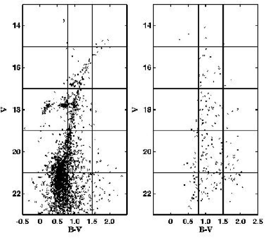
Figure 2: $(\bv,V)$ color-magnitude diagram for M75 (left panel). The field CMD (right panel) is based on images taken $30\arcmin$ east of the center of the cluster.

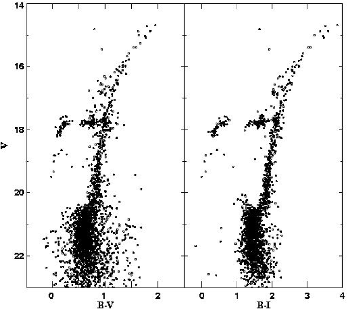
Figure 3: ($V$, $\bv$) and ($V$, $B-I$) CMDs for all stars in the NTT dataset for M75. Known variable stars are omitted from the plot.

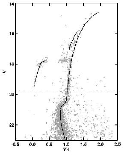
Figure 4: ($V$, $V-I$) CMD for M75, with the derived ridgeline overplotted. Crosses indicate variable stars (from Paper II). The dashed line indicates the magnitude level which separates the two samples used for better definition of the CMD branches and determination of the ridgeline: while for $V<19.7$ mag all stars were utilized (and are displayed), fainter than this level only stars with $r>150\arcsec$ were employed (and are shown). Note that, for the red HB, the “ridgeline” actually represents the lower envelope of the distribution.

3 The Color-Magnitude Diagram

3.1 Overall CMD Morphology

The ($V$, $\bv$) and ($V$, $B-I$) CMDs from the NTT dataset are presented in Fig. 3. Field stars were statistically subtracted as described in §2, and known variables are omitted from the plot.

Mean ridgelines of the main branches of M75 were determined from the ($V$, $V-I$) CMD. With this purpose, the following selection criteria were adopted in order to have the best definition of the CMD branches: for $V<19.7$ mag, all stars were used; for $V>19.7$ mag, and in order to better outline the turnoff (TO) region, only stars with $r>150\arcsec$ were employed (thus avoiding the crowding in the innermost regions while minimizing field star contamination).

The mean ridgelines of the main branches in the CMD were determined following the polynomial fitting technique by Sarajedini (1994). A first rough selection of the candidate RGB stars was performed by eye, removing the HB and part of the asymptotic giant branch (AGB) stars. A polynomial law in the form $(V-I)=F(V)$ was used. In several iterations the stars deviating by more than 2-sigma in color from the fitting relation were rejected. The standard error of the resulting fit is 0.04 mag. The mean ridgelines of the fainter part of the CMD ($V>19.7$ mag—subgiant branch and main sequence) were determined by dividing these branches into bins and computing in each bin the mode of the distribution in color. The “ridgeline” for the red HB region was determined as the lower envelope of the red clump. Table 1 presents the adopted normal points for each branch. In Fig. 4 the ($V$, $V-I$) CMD is shown with the mean ridgelines overplotted.

The main sequence (MS) TO point is found to be at $V_{\rm TO}=21.22\pm 0.09$ mag and $(V-I)_{\rm TO}=0.818\pm 0.05$ mag. The magnitude level of the HB, determined as the lower boundary of the red HB “clump,” is $V_{\rm HB}=17.80\pm 0.03$ mag. This implies a magnitude difference between the HB and the TO of $\Delta\,V^{\rm HB}_{\rm TO}=3.42\pm 0.09$ mag.

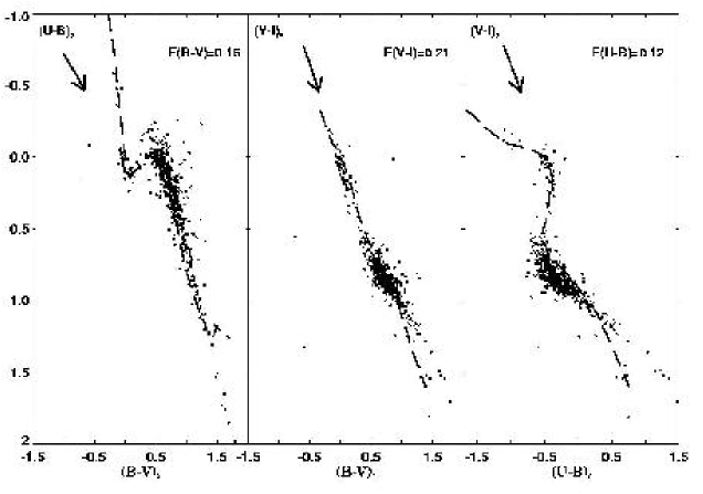
Figure 5: Dereddened color-color $(\bv)_{0}$ vs. $(U-B)_{0}$, $(\bv)_{0}$ vs. $(V-I)_{0}$, and $(U-B)_{0}$ vs. $(V-I)_{0}$ diagrams. The dashed lines are sequences of luminosity class V from Bessel (1990). The arrows show the direction of the reddening vector.

3.2 Metallicity and Reddening

The best fit of $(\bv)$ vs. $(U-B)$, $(\bv)$ vs. $(V-I)$, and $(U-B)$ vs. $(V-I)$ distributions for the M75 blue HB stars to the color-color lines from Bessel (1990) gives $E(\bv)=0.16\pm 0.02$. The fit is shown on Fig. 5.

For comparison, the Schlegel, Finkbeiner, & Davis (1998) cobe/dirbe dust maps give $E(\bv)=0.152$ mag at the M75 position, and Harris (1996) lists $E(\bv)=0.16$ mag in the latest (June 1999) version of his catalogue.

A complete set of RGB parameters and metallicity indicators in the classical $(V,\,\bv)$ plane has been recently presented by Ferraro et al. (1999a, hereafter F99). F99 also reported on an independent calibration of RGB parameters in terms of the cluster metallicity (both in the Carretta & Gratton 1997, hereafter CG97, [Fe/H] scale and in the corresponding global [M/H] scale). In particular, F99 presented a system of equations (see Table 4 in F99) which can be used to simultaneously derive an estimate of metal abundance (in terms of ${\rm[Fe/H]}_{\rm CG97}$ and [M/H]) and reddening from the morphology and location of the RGB in the $(V,\,\bv)$ CMD. The “global metallicity” [M/H] assumes an $\alpha$-element enhancement of $[\alpha/{\rm Fe}]=0.28$ for ${\rm[Fe/H]}<-1$.

For M75, we used the mean ridgeline to measure the following RGB parameters: $(\bv)_{\rm 0,g}$, defined as the RGB color at the HB level; the two RGB slopes $S_{2.0}$ and $S_{2.5}$, defined as the slope of the line connecting the intersection of the RGB and HB with the points along the RGB located, respectively, 2.0 and 2.5 mag brighter than the HB; $\Delta V_{1.1}$, $\Delta V_{1.2}$ and $\Delta V_{1.4}$—defined as magnitude differences between the HB and RGB at the fixed colors $(\bv)_{0}=1.1,1.2$ and $1.4$ mag. The derived metallicity, based on the weighted mean of the above defined values as listed in Table 2, is ${\rm[Fe/H]}_{\rm CG97}=-1.01\pm 0.12$, ${\rm[M/H]}=-0.82\pm 0.19$ and ${\rm[Fe/H]}_{\rm ZW84}=-1.22\pm 0.21$. The derived reddening is $E(\bv)=0.155\pm 0.032$. The errors associated with the measurements are conservative estimates of the global uncertainties, formal errors being much smaller than those assumed.

3.3 Red Giant Branch

The so-called RGB “bump,” corresponding to the point in the evolution of RGB stars when the H-burning shell encounters the chemical composition discontinuity left behind by the maximum inward penetration of the convective envelope, was first predicted by theoretical models (Thomas 1967; Iben 1968) and subsequently observed in many clusters (see F99 for more details). The break in the slope of the cumulative RGB luminosity function is a common technique used to locate the RGB bump (Fusi Pecci et al. 1990). The observed differential and integrated luminosity functions for the M75 RGB are shown in Fig. 6. As can be seen the RGB bump of M75 is very well defined at $V=17.75\pm 0.05$ mag.

The magnitude difference between the RGB luminosity function “bump” and the HB level, $\Delta V_{\rm HB}^{\rm bump}$, is a metallicity indicator recently recalibrated by F99. Using the data given in their Table 5 and the calibration equations from Table 6 in F99 we calculated ${\rm[Fe/H]}_{\rm CG97}=-1.10\pm 0.10$, ${\rm[M/H]}=-0.91\pm 0.09$ and ${\rm[Fe/H]}_{\rm ZW84}=-1.30\pm 0.08$. As can be seen, the RGB bump-based metallicity is in good agreement with the value derived in §3.2. A plot showing the difference in brightness between the RGB bump and the HB, $\Delta V_{\rm HB}^{\rm bump}$, as a function of metallicity is presented in Fig. 7.

Taking the RGB bump-based metallicity into account, the revised metallicity of M75, based on the weighted mean over all the values listed in Table 2, is ${\rm[Fe/H]}_{\rm CG97}=-1.03\pm 0.17$ and ${\rm[M/H]}=-0.87\pm 0.19$ on the Carretta & Gratton (1997) scale. On the Zinn & West (1984) scale we find ${\rm[Fe/H]}_{\rm ZW84}=-1.24\pm 0.21$.

Figure 6: The observed differential (upper panel) and integrated (lower panel) luminosity function for the M75 RGB.

Figure 7: The magnitude difference between the bump and the HB, $\Delta V_{\rm HB}^{\rm bump}$, as a function of [Fe/H]. Upper panel: CG97 scale; bottom panel: ZW84 scale. The filled circle indicates M75. The clusters data are from Table 5 in F99.

Figure 8: $R_{\rm bump}$ vs. global metallicity. The filled circle indicates M75.

Figure 9: The $R$-parameter, as defined by Zoccali et al. (2001), is plotted as a function of the “global metallicity.” The filled circle indicates M75. The cluster data are from Table 1 in Zoccali et al. (2001).

Recently Bono et al. (2001) defined the new parameter $R_{\rm bump}$ as the ratio between the number of stars in the bump region ($V_{\rm bump}\pm 0.4$) and the number of RGB stars in the interval $V_{\rm bump}+0.5<V<V_{\rm bump}+1.5$. In our case we calculated $R_{\rm bump}=0.47\pm 0.04$.

Comparison of the $R_{\rm bump}$ parameter with the cluster sample of Bono et al. (2001)—their Table 1—shows good agreement. In Fig. 8, where $R_{\rm bump}$ is plotted as a function of the metallicity, M75 is marked with a filled circle, showing its normal location with respect to the other clusters. This “normal” behavior of $R_{\rm bump}$ in M75, in analogy with the discussion presented by Bono et al. for the other clusters plotted in Fig. 8, suggests that the M75 bump too has not been affected by the occurrence of non-canonical deep mixing that might have substantially altered the chemical composition profile in the vicinity of the H-burning shell in the early evolution of M75’s red giants.

Harris (1975) first mentioned an abnormally high ratio $R$ of HB to red giant branch (RGB) stars. To calculate the $R$ ratio we find the following number counts: $N_{\rm HB}=149$, $N_{\rm RGB}=118$, and $N_{\rm AGB}=28$—where $N_{\rm RGB}$ is the number of RGB stars brighter than the HB level, following the definition by Buzzoni et al. (1983). The observed star counts are corrected for completeness and the estimated numbers rounded to the closest integer value. It thus follows that $R=N_{\rm HB}/N_{\rm RGB}=1.26\pm 0.15$. For $R^{\prime}=N_{\rm HB}/N_{\rm(RGB+AGB)}$, the value is $R^{\prime}=1.02\pm\,0.10$. For $R1=N_{\rm AGB}/N_{\rm RGB}$ we calculated $R1=0.24\pm\,0.05$ and $R2=N_{\rm AGB}/N_{\rm HB}$ is $R2=0.19\pm\,0.04$. We have assumed, following Buzzoni et al., a differential bolometric correction between the HB and the RGB of 0.15 mag.

If we adopt the Zoccali et al. (2001) definition of $N_{\rm RGB}$ as RGB stars brighter than the ZAHB (which is approximately equivalent to the lower envelope of the red HB), $N_{\rm RGB}$ becomes 90 (after completeness correction) and $R=1.66\pm 0.20$, $R^{\prime}=1.26\pm\,0.16$ and $R1=0.31\pm\,0.07$. Plotting the $R$ parameter vs. global metallicity in Fig. 9 (the cluster data are from Table 1 in Zoccali et al.) we can see that M75 has a high $R$ value for its metallicity—though only at the $1-2\sigma$ level.

Note that the $R$ value following the Buzzoni et al. (1983) definition does not seem atypical (or large). It is only when we use the Zoccali et al. (2001) definition that we are able to verify the suggestion by Harris (1975) of a low ratio of giants to HB stars in M75. This problem is due to the fact that the bump, at such a metallicity, is critically located close to the HB level (see Fig. 7), and may or may not be included in the number counts due to only a small change in the magnitude cutoff.

In order to further investigate this issue, we have utilized the observed RGB number counts down to a deeper magnitude level on the CMD, performing a direct comparison against similarly computed values from the theoretical simulations discussed in §3.4.1 and presented in Figs. 11 and 12 below. In order to avoid the ambiguity brought about by the positioning of the RGB bump (see Fig. 7) in the derived number counts, we define $R_{\langle M_{V}\rangle+1.0}$ and $R_{\langle M_{V}\rangle+1.5}$ as the ratio between HB stars and RGB stars brighter than $\langle M_{V}({\rm HB})\rangle+1$ mag and $\langle M_{V}({\rm HB})\rangle+1.5$ mag, respectively. The resulting comparison between the observed and theoretical number ratios is given in Table 3. As can be seen, the observed $R$-ratios are clearly confirmed to be higher than the values predicted for $Y_{\rm MS}=0.23$, in agreement with the conclusion based on the Zoccali et al. (2001) definition of the $R$-ratio and with the original suggestion by Harris (1975) that M75 seems to have too few giants compared to HB stars.

What is the origin of the larger $R$-ratio for M75? The traditional explanation would involve a larger helium abundance for this cluster (Iben 1968). Is this a viable explanation, in the case of M75? In order to answer this question, we may take benefit of the predicted dependence of HB luminosity on the helium abundance, which should accordingly lead to longer periods for M75’s RR Lyrae variables (e.g., Catelan 1996). We will check whether this is the case, or whether other explanations are required, in Paper II, where we present a detailed analysis of the M75 RR Lyrae light curves.

3.4 HB Morphology

3.4.1 HB Multimodality

Fig. 10 shows the HB region of the CMD of M75 in several different planes: ($V$, $U-V$); ($V$, $U-I$); and ($U$, $U-V$). Known variable stars (see Paper II) are omitted from these plots. Both the red and the blue HB regions are very well populated, as first noted by Harris (1975). The blue part of the HB has a blue tail and an obvious “gap” at $V\simeq 18.5$ mag and $(U-V)_{0}$ between $-0.55$ and $-0.15$, corresponding to temperatures in the range $10,\!500\lesssim T_{\rm eff}({\rm K})\lesssim 13,\!500$—which overlaps the suggested “G1” and “G2” gaps in Ferraro et al. (1998). Another, much less obvious gap (or underpopulated region) may be present at $V\approx 17.9-18.0$ mag and $(U-V)_{0}\approx 0.1$ mag, $(B-I)_{0}\approx 0.1$ mag.

In order to more quantitatively describe the morphology of the HB, we computed several useful HB morphology parameters, including those defined by Mironov (1972), Zinn (1986), Lee, Demarque, & Zinn (1990), Buonanno (1993), Fusi Pecci et al. (1993), and Catelan et al. (2001b). Several of these authors have emphasized the importance of utilizing as many HB morphology parameters as possible when drawing general inferences based on the HB morphology of Galactic GCs. The values of the computed parameters are given in Table 4. We briefly recall that $B$, $V$, and $R$ are the number of blue HB, variable (RR Lyrae), and red HB stars, respectively; $B2$ is the number of blue HB stars bluer than $(\bv)_{0}=-0.02$ mag; $B2^{\prime}$ is the number of HB stars redder than $(V-I)_{0}=-0.02$ mag; $B7^{\prime}$ is the number of blue HB stars redder than $(V-I)_{0}=+0.07$ mag; and, finally, $B0^{\prime}$ is the number of blue HB stars redder than $(V-I)_{0}=0.0$ mag.

To compute the reddening-dependent HB morphology parameters, we have assumed $E(\bv)=0.16$ (§3). Also, the number of variable stars, $V=22$, was adopted from our comprehensive variability survey, described in Paper II. All observed number counts are corrected for completeness.

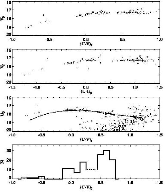
Figure 10: Zoomed ($V$, $U-V$), ($V$, $U-I$) and ($U$, $U-I$) CMDs of M75 around the HB region. The bottom panel shows a histogram of the $(U-V)_{0}$ color distribution for M75 HB stars. In this panel, the RR Lyrae region is indicated with a dashed line; the $(U-V)_{0}$ color distribution of the M75 RR Lyrae was assumed to be approximately uniform.

It is obvious from these numbers that M75 is indeed another cluster with a strongly bimodal HB, since it has many fewer RR Lyrae variables than either red HB or blue HB stars. A histogram with the $(U-V)_{0}$ color distribution of the M75 HB stars (corrected for completeness) is given in the bottom panel of Fig. 10. Since we do not have $U-V$ mean colors for the variables we assume a flat distribution. This clearly shows that the distribution of stars along the HB of M75 has three main modes—though the third mode, on the blue tail, is very thinly populated. For a detailed discussion of the completeness of our RR Lyrae search, see Paper II.

The M75 HB clearly bears striking resemblance to that of the well-known bimodal-HB GC NGC 1851, as first pointed out by Catelan et al. (1998a) on the basis of the Harris (1975) photographic CMD. In particular, the number ratios $B:\,V:\,R=0.38:\,0.16:\,0.45$ are similar to those for NGC 1851, for which $B:\,V:\,R=0.30:\,0.10:\,0.60$.

We have investigated further the issue of HB bimodality in M75 by computing a new grid of synthetic HBs aimed at matching the HB morphology parameters displayed in Table 4. Our purpose is to check whether a bimodality in the underlying evolutionary parameters is necessarily implied by the observed bimodality in the HB number counts (Catelan et al. 1998a). Our simulations, computed with sintdelphi (Catelan et al. 2001b), utilize the evolutionary tracks for $Y_{\rm MS}=0.23$, $Z=0.002$ from Sweigart & Catelan (1998). Observational scatter has been added by means of suitable analytical representations of the errors in the photometry. The number of HB stars in these simulations is similar to the observed one, $N_{\rm HB}=149$, but has been allowed to fluctuate according to the Poisson distribution.

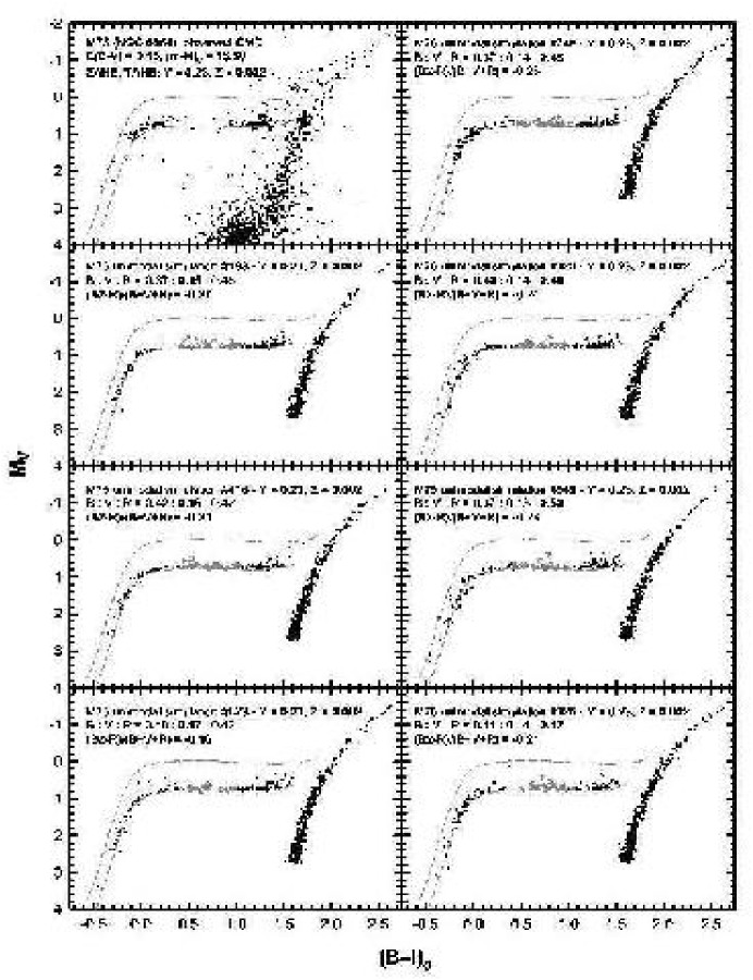
Figure 11: Random sample of HB simulations for M75 in the unimodal ZAHB mass distribution case. The $M_{V}$, $(B-I)_{0}$ plane is shown. We have assumed $E(B-I)/E(\bv)=2.7$, after Stetson (1998). In the upper left panel, the observational data are shown, along with the reddening value and distance modulus found more suitable to fit the theoretical ZAHB for the indicated chemical composition to the observed distribution. Variable stars are omitted in the panel showing the observed CMD, but not in the others (where they are displayed as encircled gray dots)—which show the theoretical CMD simulations. Also indicated are the $B:V:R$ number ratios and the value of the Buonanno (1993) HB morphology parameter.

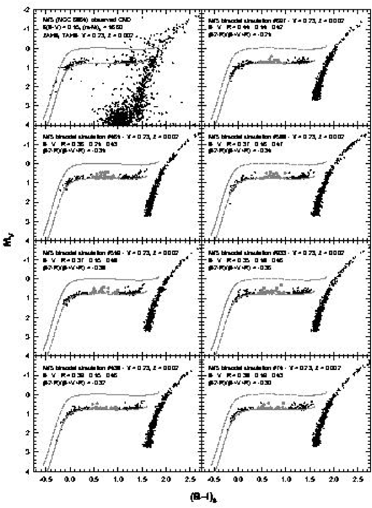
Figure 12: As in Fig. 11, but for the bimodal mass distribution case.

We first attempted to reproduce the observed HB morphology parameters for M75 by means of a unimodal Gaussian deviate in the zero-age HB (ZAHB) mass. Following a procedure similar to that described in Catelan et al. (2001a, 2001b), we find a best match between the observed and predicted HB morphology parameters for $\langle M_{\rm HB}\rangle=0.624\,M_{\sun}$, $\sigma_{M}=0.043\,M_{\sun}$. Some randomly selected samples of simulations for this unimodal mass distribution case are displayed, in the [$M_{V}$, $(B-I)_{0}$] plane, in Fig. 11. The predicted HB morphology parameters for this case are shown in Table 4 (third column); the indicated “error bars” represent the standard deviation of the mean over a set of 1000 simulations. It is readily apparent that, while the overall general agreement, particularly in terms of the commonly employed Mironov and Lee-Zinn parameters, is reasonable, some of the other parameters introduced by Catelan et al., especially $B0^{\prime}/B$ and $B7^{\prime}/(B+V+R)$, are not accounted for in an entirely satisfactory way by these simulations. For this reason, we have attempted to compute extra sets of simulations for an intrinsically bimodal distribution in mass on the ZAHB.

In the bimodal case, we have found that the following combination of parameters gives the best fit between the models and the observations: $\langle M_{\rm HB,1}\rangle=0.595\,M_{\sun}$, $\sigma_{M,1}=0.010\,M_{\sun}$, $N_{\rm HB,1}=46$; $\langle M_{\rm HB,2}\rangle=0.640\,M_{\sun}$, $\sigma_{M,2}=0.030\,M_{\sun}$, $N_{\rm HB,2}=104$. Some randomly selected samples of simulations for this bimodal mass distribution case are displayed, in the [$M_{V}$, $(B-I)_{0}$] plane, in Fig. 12. The predicted HB morphology parameters for this case are also shown in Table 4 (fourth column).

We find that the intrinsically bimodal mass distribution case provides a much more satisfactory fit to the whole set of HB morphology parameters than does the unimodal case. To some extent, this is not an unexpected result, given that this case contains five free parameters, as opposed to two in the unimodal one (Catelan et al. 1998a). The main difference between the bimodal and unimodal cases, as can be readily appreciated by inspection of Figs. 11 and 12, is that the unimodal case clearly predicts that a fairly extended blue tail should be present in M75, whereas this is not necessarily required in the bimodal case. Also in this respect, apart from a few cases where statistical fluctuations change the predicted simulations quite substantially, the bimodal case appears much more successful at matching the observed distribution, showing, in general, a more stubby blue HB with relatively few hot stars being in general expected. Note, however, that neither the unimodal nor the bimodal cases shown in Figs. 11 and 12 can successfully account for the existence of a third mode of hotter HB stars along the blue tail of M75 (see also Fig. 10, bottom panel).

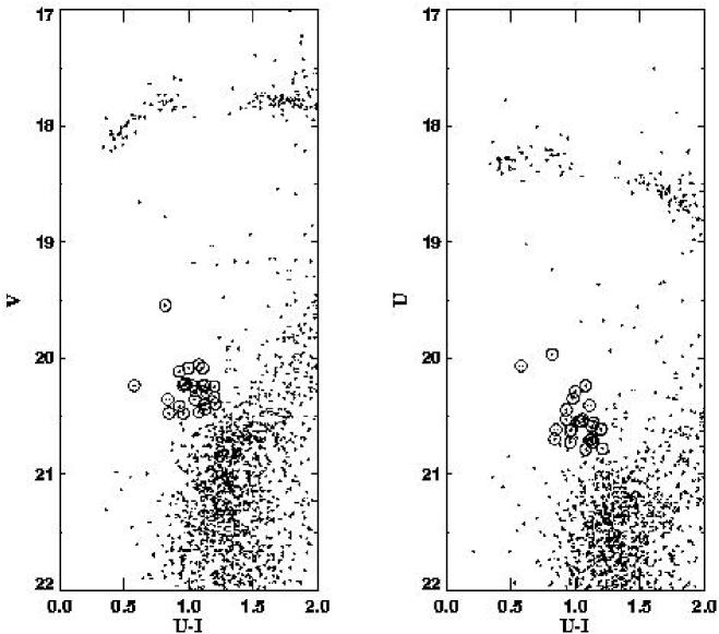
Figure 13: Zoomed ($U-I$, $V$) and ($U-I$, $U$) CMDs of the BSS region (left and right panels, respectively). Candidate BSS are plotted as encircled dots.

Figure 14: Radial cumulative distributions of the candidate BSS (circles) and SGB stars (diamonds) in M75.

3.4.2 The Grundahl Jump in Broadband $U$

Grundahl et al. (1999) have recently shown that the interpretation of Strömgren $u$ photometry of blue HB stars in GCs is affected by a most intriguing phenomenon: at temperatures higher than $T_{\rm eff}\approx 11,\!500$ K, all GC CMDs show an intriguing “jump” in the $u$, $(u-y)_{0}$ plane, with all blue HB stars hotter than 11,500 K appearing brighter and/or hotter than predicted by the models. As argued by Grundahl et al., and spectacularly confirmed by Behr et al. (1999), the reason for this discrepancy can be attributed to the fact that the atmospheres of hot HB stars in GCs are affected by radiative levitation of metals, which pumps up heavy metals to supersolar levels in these stars’ atmospheres.

As can be seen in Fig. 10 (bottom panel), a similar jump is present also in broadband $U$, with all stars blueward than $(U-V)_{0}=-0.5$ falling systematically above the canonical ZAHB. The displayed ZAHB sequence corresponds to VandenBerg et al. (2000) models for ${\rm[Fe/H]}=-1.14$ and $[\alpha/{\rm Fe}]=+0.3$, and were transformed to the observational plane using standard prescriptions from Kurucz (1992)—which assume that the cluster metallicity is appropriate also for the atmospheres of hotter blue HB stars. It is worth noting that the Grundahl jump phenomenon in broadband $U$ has recently been verified also by Siegel et al. (1999), Bedin et al. (2000), and Markov, Spassova, & Baev (2001). The presence of the jump phenomenon in broadband $U$ is in good agreement with the radiative levitation scenario, as can be seen from inspection of Fig. 7 in Grundahl et al. (1999).

3.5 Blue Straggler Stars

On the basis of their location in the ($V$, $U-I$) CMD, we identified a sample of 26 candidate BSS. The $x$ and $y$ coordinates (in pixels) and $U$, $B$, $V$, $I$ magnitudes and distance from the cluster center (in arcmin) for these candidate BSS are listed in Table 5.

Fig. 13 shows zoomed M75 CMDs where the BSS candidates are plotted as encircled dots. As can be seen, all the candidates selected in the ($V$, $U-I$) plane lie also in the BSS region in the ($U$, $U-I$) CMD. Moreover, the latter CMD suggests that a few additional objects might be considered BSS candidates. We conservatively decided, however, to limit our analysis to those stars which are BSS candidates in both the indicated CMDs.

Careful checks were made to ensure that the internal errors of the BSS candidates are the same as those of the subgiant branch (SGB) stars at the same brightness level. The daophot parameters sharp and chi were checked for each BSS candidate, in order to ensure that most are unlikely to be the result of spurious photometric blends (e.g., Ferraro, Fusi Pecci, & Buonanno 1992). The positions of the BSS were checked on the statistically decontaminated CMDs. The number of field stars is not sufficient to explain the BSS population (see also Fig. 2).

In order to quantitatively compare the BSS populations among different Galactic GCs, one needs to suitably normalize the numbers of such stars. In this sense, Ferraro et al. (1999b) defined the specific fraction of BSS as the number of BSS normalized to the number of HB stars observed in the same cluster region, $F_{\rm HB}^{\rm BSS}=N_{\rm BSS}/N_{\rm HB}$. In M75, the specific frequency calculated in this way is $F_{\rm HB}^{\rm BSS}\simeq 0.15$.

Generally, BSS are more centrally concentrated with respect to the other stars in the cluster, although there are notable exceptions to this general rule, such as M3 (Ferraro et al. 1993, 1997) and M13 (Paltrinieri et al. 1998). In M75 we compared the radial distribution of BSS with respect to SGB stars (in the range $19.5<V<20.5$). The cumulative radial distributions are plotted, as a function of the projected distance ($r$) from the cluster center, in Fig. 14, where one sees that the M75 BSS (circles) are more centrally concentrated than the SGB sample (diamonds). The Kolmogorov-Smirnov test shows that the probability of drawing the two populations from the same distribution is $0.3\%$.

4 Age Determination

Two main methods are currently used to measure relative ages: (i) the so-called vertical method—based on the TO luminosity with respect to the HB level (Buonanno, Corsi, & Fusi Pecci 1989) and (ii) the horizontal method—based on the accurate determination of the color difference $\Delta(\bv)_{\rm TO}^{\rm RGB}$ between the base of the RGB and the TO (VandenBerg, Bolte, & Stetson 1990).

Admittedly, our photometry in the [$(\bv)$, $V$] plane is not sufficiently accurate to derive precise color difference measures down to the TO region. In addition, the horizontal method is so intrinsically sensitive to small variations in colour that even small ($\sim 0.01$ mag) uncertainties in the registration of the mean ridge lines could generate large ($\sim 1$ Gyr), “artificial” differences in the derived ages. For this reason, in order to obtain a relative age for M75, we applied only the vertical method.

In doing this, we perform a comparison with respect to another cluster with similar metallicity and HB morphology—namely, NGC 1851. Recent photometry in the [$(V-I)$, $V$] plane has been published for NGC1851 by Bellazzini et al. (2001). In Fig. 15 the fiducial lines of NGC 1851 (from Bellazzini et al.) are overplotted on the CMD of M75 in the [$(V-I)_{0}$, $V$] plane.

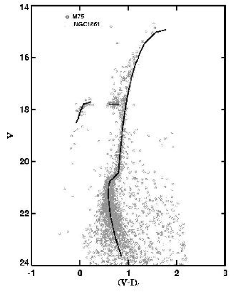
Figure 15: The [$(V-I)_{0}$, $V$] CMD of M75 with the fiducial line of NGC 1851 (from Bellazzini et al. 2001) overplotted (solid lines).

As can be seen from Fig. 15, while both the HB and the SGB/TO regions of the two clusters nicely agree, a small difference in colour in the brightest region of the RGB does exist between the two data sets. This small colour residual could in principle be due to a small difference in the global metallicity between the two clusters, although the metallicity value derived in §3.2 for M75 is very similar to that from Ferraro et al. (1999) for NGC 1851. In our opinion, the noted mismatch is likely due to a not completely accounted for “colour equation” in one of the two datasets. This effect is generally due to poor coverage in colour of the standard stars.

On the basis of the VandenBerg & Bell (1985) models, Buonanno et al. (1993) obtained the following “vertical” relation between the differential age parameter $\Delta=\Delta_{1}V_{\rm TO}^{\rm HB}-\Delta_{2}V_{\rm TO}^{\rm HB}$ and the age $t_{9}$ in Gyr:

$$\Delta\log t_{9}=(0.44+0.04\,{\rm[Fe/H]})\,\Delta.$$ (1)

In our case, we shall assume that subscript “1” stands for M75, and “2” for NGC 1851. For NGC 1851 we used the data given in Bellazzini et al. (2001) to find $\Delta V_{\rm TO}^{\rm HB}=3.43\pm 0.1$. Assuming ${\rm[Fe/H]}\simeq-1.05$ for both M75 (§3.2) and NGC 1851 and using the value of $\Delta V_{\rm TO}^{\rm HB}$ derived in §3.1 for M75, we obtain $\Delta=3.42-3.43=-0.01\pm 0.1$ mag, implying $\Delta\log t_{9}\sim-0.004$ and thus

$$\Delta\,t_{9}({\rm M75}-{\rm NGC\,1851})\sim-0.1\pm 2.0\,\,{\rm Gyr}.$$

This result suggests that M75 is essentially coeval with NGC 1851. For recent comparisons of the age of NGC 1851 with that of other GCs with similar metallicity, including NGC 288 and NGC 362, the reader is referred to Rosenberg et al. (1999), VandenBerg (2000), and Bellazzini et al. (2001); these papers all seem to indicate that NGC 1851 is (slightly) younger than other GCs of similar metallicity.

We note that even though the Buonanno et al. (1993) formula, Eq. (1) above, is not based on the latest evolutionary models available in the literature, they are still expected to give sufficiently accurate relative ages, under the hypothesis that both clusters have the same chemical composition.

5 Summary and Concluding Remarks

In this paper, we have provided the first CCD photometry for the distant GC M75. We confirm a previous suggestion (Catelan et al. 1998a) that this cluster contains two main modes on the HB, and show that the cluster actually has a third mode on the blue tail, clearly separated from the bulk of the blue HB by a wide gap, encompassing about 3000 K in temperature. In CMDs utilizing broadand $U$ magnitudes, these hotter HB stars are found to be clearly inconsistent with canonical evolutionary models, showing that the “Grundahl jump” phenomenon (Grundahl et al. 1999) can be studied using broadband $U$ besides Strömgren $u$. We also find a population of centrally concentrated BSS in M75. The metallicity inferred for this cluster from our photometry, ${\rm[Fe/H]}=-1.03\pm 0.17$ in the CG97 scale and ${\rm[Fe/H]}=-1.24\pm 0.21$ in the ZW84 scale, is similar to that of the well-known bimodal-HB globular NGC 1851, thus enabling a straightforward comparison of their turnoff ages. We find that the two clusters have essentially the same age. This is an interesting result, in view of the fact that NGC 1851 itself has been argued to be slightly younger than other GCs of similar metallicity (Bellazzini et al. 2001 and references therein). However, better photometry is needed to conclusive demonstrate that M75 too is younger than the average for its metallicity.

What is the physical reason for the HB multimodality in M75? At present, this remains unclear. Similar anomalies in HB morphology have been seen in other clusters, and the suggested explanations—none of which is seemingly capable of accounting for all the peculiarities—usually involve environmental effects, stellar rotation, abundance anomalies, mass loss in RGB stars, binarity, and even planets (e.g., Sosin et al. 1997 and references therein). In the case of M75, we are in a bad position to analyze most of these factors, given the lack of spectroscopic data for the cluster stars.

However, at least as far as the HB bimodality (i.e., relative absence of RR Lyrae stars, compared with both blue and red HB stars) is concerned, we can make use of RR Lyrae pulsation properties in order to investigate the presence of any non-canonical effects that might impact their pulsational properties in a significant way. This could at least differentiate processes which affect HB morphology by means solely of RGB mass loss from those that may affect not only the HB star masses, but also their luminosities (Catelan, Sweigart, & Borissova 1998b). Similarly, useful constraints can thereby be placed on the origin of M75’s peculiar $R$-ratio.

With this in mind, we undertook an extensive variability survey of M75. In Paper II we will provide a detailed discussion of the variable stars population in this cluster, in the hope that this will help us better understand the possible origin(s) of its peculiar HB morphology. Accordingly, a more extensive discussion of possible explanations for M75’s peculiar HB will also be deferred to Paper II.

Table 1: Mean Fiducial Lines for M75

$V$	$V-I$	$V$	$V-I$	$V$	$V-I$
MS+SGB+RGB
14.58	1.954	20.83	0.842	17.81	0.33
14.86	1.750	20.90	0.831	17.88	0.26
15.40	1.537	20.95	0.828	17.98	0.24
15.75	1.447	21.01	0.822	18.12	0.22
16.25	1.338	21.12	0.819	18.80	0.12
16.75	1.262	21.22	0.818	19.15	0.08
17.25	1.200	21.30	0.819	19.45	0.06
17.75	1.149	21.40	0.819	AGB
18.25	1.110	21.50	0.822	15.84	1.32
18.75	1.079	21.64	0.829	16.13	1.24
19.25	1.048	21.78	0.839	16.41	1.19
19.72	1.026	21.93	0.850	16.72	1.12
20.00	1.014	22.06	0.861	17.15	1.07
20.10	1.010	22.33	0.889
20.20	1.006	22.72	0.932
20.30	1.003	23.05	0.978
20.39	0.997	Red HB
20.47	0.988	17.80	1.00
20.54	0.970	17.80	0.90
20.60	0.946	17.80	0.80
20.65	0.915	17.80	0.70
20.70	0.884	Blue HB
20.75	0.862	17.80	0.40

Table 2: M75 Metallicity

Parameter	[Fe/H]
CG97 scale
$(\bv)_{0,{\rm g}}$	$-1.21\pm 0.22$
$\Delta V_{1.1}$	$-0.95\pm 0.16$
$\Delta V_{1.2}$	$-0.92\pm 0.14$
$\Delta V_{1.4}$	$-0.97\pm 0.12$
$S_{2.5}$	$-0.74\pm 0.19$
$S_{2.0}$	$-0.74\pm 0.19$
$\Delta V_{\rm HB}^{\rm bump}$	$-1.10\pm 0.10$
ZW84 scale
$(V-B)_{0,{\rm g}}$	$-1.29\pm 0.15$
$\Delta V_{1.1}$	$-1.21\pm 0.14$
$\Delta V_{1.2}$	$-1.16\pm 0.21$
$\Delta V_{\rm HB}^{\rm bump}$	$-1.30\pm 0.13$

Table 3: Ratio between HB and RGB Stars in M75

Parameter	Observed	Model, Unimodal	Model, Bimodal
$R_{\langle M_{V}\rangle}$	$1.75\pm 0.20$	$1.52\pm 0.20$	$1.52\pm 0.20$
$R_{\langle M_{V}\rangle+1.0}$	$0.89\pm 0.12$	$0.73\pm 0.08$	$0.73\pm 0.08$
$R_{\langle M_{V}\rangle+1.5}$	$0.80\pm 0.09$	$0.51\pm 0.05$	$0.51\pm 0.05$

Table 4: HB Morphology Parameters for M75

Parameter	Observed	Model, Unimodal	Model, Bimodal
$B:\,V:\,R$	$0.38:\,0.16:\,0.45$	$0.369:\,0.164:\,0.467$	$0.374:\,0.162:\,0.463$
		$(0.040)\,(0.030)\,(0.040)$	$(0.040)\,(0.030)\,(0.039)$
$B/(B+R)$	$+0.46\pm 0.05$	$+0.442\pm 0.045$	$+0.447\pm 0.044$
$(B-R)/(B+V+R)$	$-0.07\pm 0.03$	$-0.097\pm 0.075$	$-0.089\pm 0.073$
$(B2-R)/(B+V+R)$	$-0.29\pm 0.05$	$-0.251\pm 0.064$	$-0.332\pm 0.056$
$B2^{\prime}/(B+V+R)$	$+0.94\pm 0.11$	$+0.820\pm 0.032$	$+0.924\pm 0.022$
$B7^{\prime}/(B+V+R)$	$+0.15\pm 0.05$	$+0.099\pm 0.025$	$+0.150\pm 0.029$
$B0^{\prime}/B$	$+0.65\pm 0.13$	$+0.449\pm 0.068$	$+0.705\pm 0.063$

Table 5: BSS Candidates

$x$	$y$	$U$	$B$	$V$	$I$	$r(\arcmin)$
858.487	928.874	20.726	21.033	20.234	19.765	1.197
1569.31	509.059	20.706	20.695	20.234	19.595	3.174
856.750	1025.86	19.966	20.005	19.544	19.145	1.083
642.167	1130.38	20.616	20.649	20.224	19.645	2.060
1043.11	561.039	20.776	21.033	20.394	19.565	2.182
1221.19	994.192	20.616	20.954	20.244	19.415	0.591
1029.49	361.2	20.586	20.739	20.234	19.455	3.069
393.541	354.62	20.696	20.779	20.354	19.855	4.394
969.387	756.66	20.446	0	20.114	19.515	1.423
1380.32	889.383	20.786	20.961	20.464	19.705	1.432
664.147	1643.63	20.406	20.527	20.084	19.295	3.264
1245.00	1180.94	20.546	0	20.234	19.515	0.866
903.636	1184.78	20.696	20.855	20.394	19.565	1.055
908.318	665.808	20.696	0	20.404	19.575	1.903
1211.07	1287.94	20.726	20.744	20.434	19.595	1.164
1416.58	662.593	20.606	0	20.334	19.405	2.218
1342.55	1132.68	20.556	20.666	20.294	19.415	1.136
1078.26	1238.95	20.526	20.629	20.284	19.465	0.843
1117.41	1278.94	20.286	20.429	20.084	19.285	1.017
1200.79	512.574	20.546	20.699	20.354	19.495	2.424
668.343	1009.46	20.236	20.31	20.054	19.155	1.922
1272.36	1202.11	20.626	0	20.474	19.665	1.019
1203.81	1231.74	20.616	20.748	20.474	19.765	0.927
1092.07	1312.79	20.346	20.39	20.214	19.365	1.165
972.800	771.894	20.526	0	20.414	19.595	1.355
1239.57	852.423	20.066	0	20.234	19.485	1.072

References

- (1)
- (2) Alvarado, F., Wenderoth, E., Alcaino, G., & Liller, W. 1990, AJ, 99, 1501
- (3)
- (4) Bedin, L. R., Piotto, G., Zoccali, M., Stetson, P. B., Saviane, I., Cassisi, S., & Bono, G. 2000, A&A, 363, 159
- (5)
- (6) Behr, B. B., Cohen, J. G., McCarthy, J. K., & Djorgovski, S. G. 1999, ApJ, 517, L135
- (7)
- (8) Bellazzini, M., Fusi Pecci, F., Ferraro, F. R., Galleti, S., Catelan, M., & Landsman, W. B. 2001, AJ, 122, 2569
- (9)
- (10) Bessel, M. S. 1990, PASP, 102, 1181
- (11)
- (12) Bono, G., Cassisi, S., Zoccali, M., & Piotto, G. 2001, ApJ, 546, L109
- (13)
- (14) Borissova, J., Catelan, M., Spassova, N., & Sweigart, A. V., 1997, AJ, 113, 692
- (15)
- (16) Buonanno, R. 1993, in ASP Conf. Ser. Vol. 48, The Globular Cluster-Galaxy Connection, ed. G. H. Smith & J. P. Brodie (San Francisco: ASP), 131
- (17)
- (18) Buonanno, R., Corsi, C. E., & Fusi Pecci, F. 1989, A&A, 216, 80
- (19)
- (20) Buonanno, R., Corsi, C. E., Fusi Pecci, F., Richer, H. B., & Fahlman, G. G. 1993, AJ, 105, 184
- (21)
- (22) Carretta, E., & Gratton, R. 1997, A&AS, 121, 95 (CG97)
- (23)
- (24) Catelan, M. 1996, A&A, 307, L13
- (25)
- (26) Catelan, M. 2000, ApJ, 531, 826
- (27)
- (28) Catelan, M., Bellazzini, M., Landsman, W. B., Ferraro, F. R., Fusi Pecci, F., & Galleti, S. 2001a, AJ, 122, 3171
- (29)
- (30) Catelan, M., Borissova, J., Sweigart, A. V., & Spassova, N. 1998a, ApJ, 494, 265
- (31)
- (32) Catelan, M., Ferraro, F. R., & Rood, R. T. 2001b, ApJ, 560, 970
- (33)
- (34) Catelan, M., Sweigart, A. V., & Borissova, J. 1998b, in ASP Conf. Ser. Vol. 135, A Half-Century of Stellar Pulsation Interpretations, ed. P. A. Bradley & J. A. Guzik (San Francisco: ASP), 41
- (35)
- (36) Corwin, T. M., Catelan, M., Smith, H. A., Borissova, J., & Ferraro, F. R. 2001, AJ, in preparation (Paper II)
- (37)
- (38) Ferraro, F. R., et al. 1997, A&A, 324, 915
- (39)
- (40) Ferraro, F. R., Fusi Pecci, F., & Buonanno, R. 1992, MNRAS, 256, 376
- (41)
- (42) Ferraro, F. R., Fusi Pecci, F., Cacciari, C., Corsi, C. E., Buonanno, R., Fahlman, G. G., & Richer, H. B. 1993, AJ, 106, 2324
- (43)
- (44) Ferraro, F. R., Messineo, M., Fusi Pecci, F., De Palo, M. A., Straniero, O., Chieffi, A., & Limongi, M. 1999a, AJ, 118, 1738 (F99)
- (45)
- (46) Ferraro, F. R., Paltrinieri, B., Fusi Pecci, F., Rood, R. T., & Dorman, B. 1998, ApJ, 500, 311
- (47)
- (48) Ferraro, F. R., Paltrinieri, B., Rood, R. T., & Dorman, B. 1999b, ApJ, 522, 983
- (49)
- (50) Fusi Pecci, F., & Bellazzini, M. 1997, in The Third Conference on Faint Blue Stars, ed. A. G. Davis Philip, J. W. Liebert, & R. A. Saffer (Schenectady: L. Davis Press), 255
- (51)
- (52) Fusi Pecci, F., Bellazzini, M., Djorgovski, S., Piotto, G., & Buonanno, R. 1993, AJ, 105, 1145
- (53)
- (54) Fusi Pecci, F., Ferraro, F. R., Crocker, D. A., Rood, R. T., & Buonanno, R. 1990, A&A, 238, 95
- (55)
- (56) Grundahl, F., Catelan, M., Landsman, W. B., Stetson, P. B., & Andersen, M. I. 1999, ApJ, 524, 242
- (57)
- (58) Harris, W. E. 1975, ApJS, 29, 397
- (59)
- (60) Harris, W. E. 1996, AJ, 112, 1487 (June 22nd, 1999 version)
- (61)
- (62) Iben, I., Jr. 1968, Nature, 220, 143
- (63)
- (64) Kraft, R. P., Sneden, C., Smith, G. H., Shetrone, M. D., & Fulbright, J. 1998, AJ, 115, 1500
- (65)
- (66) Kurucz, R. L. 1992, in IAU Symp. 149, The Stellar Populations of Galaxies, ed. B. Barbuy & A. Renzini (Dordrecht: Kluwer), 225
- (67)
- (68) Lee, Y.-W., Demarque, P., & Zinn, R. 1990, ApJ, 350, 155
- (69)
- (70) Lee, Y.-W., Demarque, P., & Zinn, R. 1994, ApJ, 423, 248
- (71)
- (72) Majewski, S. R. 1994, ApJ, 431, L17
- (73)
- (74) Markov, H., Spassova, N., & Baev, P. 2001, MNRAS, 326, 102
- (75)
- (76) Mironov, A. V. 1972, AZh, 49, 134
- (77)
- (78) Paltrinieri, B., Ferraro, F. R., Fusi Pecci, F., & Carretta, E. 1998, MNRAS, 293, 434
- (79)
- (80) Pryor, C., & Meylan, G. 1993, in ASP Conf. Ser. Vol. 50, Structure and Dynamics of Globular Clusters, ed. S. Djorgovski & G. Meylan (San Francisco: ASP), 357
- (81)
- (82) Rich, R. M., et al. 1997, ApJ, 484, L25
- (83)
- (84) Rood, R. T., Crocker, D. A., Fusi Pecci, F., Ferraro, F. R., Clementini, G., & Buonanno, R. 1993, in ASP Conf. Ser. Vol. 48, The Globular Cluster-Galaxy Connection, ed. G. H. Smith & J. P. Brodie (San Francisco: ASP), 218
- (85)
- (86) Rosenberg, A., Saviane, I., Piotto, G., & Aparicio, A. 1999, AJ, 118, 2306
- (87)
- (88) Sandage, A., & Wildey, R. 1967, ApJ, 150, 469
- (89)
- (90) Sarajedini, A. 1994, AJ, 107, 618
- (91)
- (92) Sarajedini, A., Chaboyer, B., & Demarque, P. 1997, PASP, 109, 1321
- (93)
- (94) Saviane, I., Rosenberg, A., Piotto, G., & Aparicio, A. 2000, A&A, 355, 966 (S00)
- (95)
- (96) Schlegel, D. J., Finkbeiner, D. P., & Davis, M. 1998, ApJ, 500, 525
- (97)
- (98) Searle, L., & Zinn, R. 1978, ApJ, 225, 357
- (99)
- (100) Siegel, M. H., Majewski, S. R., Catelan, M., & Grundahl, F. 1999, BAAS, 195, #131.01
- (101)
- (102) Soker, N. 1998, AJ, 116, 1308
- (103)
- (104) Soker, N., & Harpaz, A. 2000, MNRAS, 317, 861
- (105)
- (106) Sosin, C., et al. 1997, ApJ, 480, L35
- (107)
- (108) Stetson, P. B. 1991a, in ASP Conf. Ser. Vol. 13, The Formation and Evolution of Star Clusters, ed. K. A. Janes (San Francisco: ASP), 88
- (109)
- (110) Stetson, P. B. 1991b, in Precision Photometry: Astrophysics of the Galaxy, ed. A. G. D. Philip, A. R. Upgren, & K. A. Janes (Schenectady: L. Davis Press), 69
- (111)
- (112) Stetson, P. B. 1993, User’s Manual for daophot ii
- (113)
- (114) Stetson, P. B. 1998, CFHT Bull., 38, 1
- (115)
- (116) Stetson, P. B., & Harris, W. E. 1988, AJ, 96, 909
- (117)
- (118) Stetson, P. B., VandenBerg, D. A., & Bolte, M. 1996, PASP, 108, 560
- (119)
- (120) Sweigart, A. V. 1997a, ApJ, 474, L23
- (121)
- (122) Sweigart, A. V., 1997b, in The Third Conference on Faint Blue Stars, ed. A. G. D. Philip, J. Liebert, & R. A. Saffer (Cambridge: Cambridge University Press), 3
- (123)
- (124) Sweigart, A. V., & Catelan, M. 1998, ApJ, 501, L63
- (125)
- (126) Thomas, H.-C. 1967, Z. Astrophys., 67, 420
- (127)
- (128) van den Bergh, S. 1993, ApJ, 411, 178
- (129)
- (130) VandenBerg, D. A. 2000, ApJS, 129, 315
- (131)
- (132) VandenBerg, D. A., & Bell, R. A. 1985, ApJS, 58, 561
- (133)
- (134) VandenBerg, D. A., Bolte, M., & Stetson, P. B. 1990, AJ, 100, 445
- (135)
- (136) VandenBerg, D. A., & Stetson, P. B. 1991, AJ, 102, 1043
- (137)
- (138) VandenBerg, D. A., Swenson, F. J., Rogers, F. J., Iglesias, C. A., & Alexander, D. R. 2000, ApJ, 532, 430
- (139)
- (140) Walker, A. R. 1998, AJ, 116, 220
- (141)
- (142) Zinn, R. 1986, in Stellar Populations, ed. C. A. Norman, A. Renzini, & M. Tosi (Cambridge: Cambridge University Press), 73
- (143)
- (144) Zinn, R. 1993, in ASP Conf. Ser. Vol. 48, The Globular Cluster–Galaxy Connection, ed. G. A. Smith & J. P. Brodie (San Francisco: ASP), 38
- (145)
- (146) Zinn, R., & West, M. J. 1984, ApJS, 55, 45 (ZW84)
- (147)
- (148) Zoccali, M., Cassisi, S., Bono, G., Piotto, G., Rich, R., & Djorgovski, S., 2000, ApJ, 538, 289
- (149)