Enhancement of $\alpha$-Elements in Dynamical Models of Elliptical Galaxies

In this paper we present a quantitative analysis of the chemical abundances in ”monolithic” N-body-Tree-SPH models of elliptical galaxies to determine whether the ratio [$\alpha$/Fe] increases with the galaxy mass as suggested by observational data.

1 Introduction

Twenty years after the seminal papers on the formation of elliptical galaxies (EGs) by Larson (1975) and Toomre (1977) there is still much disagreement among astronomical community on both the process of formation and evolution of early-type galaxies.

Are EGs formed in a single collapse during a short epoch of activity (monolithic scheme) or continuously by hierarchical mergers at similar levels by several mergers (hierarchical scheme)? Once created, is the stellar population of EGs just passively evolving or do minor merging/accretion events drastically change their characteristics frequently? What is the influence of density environment?

In the monolithic scenario EGs are supposed to suffer dominant star forming activity and consequent chemical enrichment at very early epochs followed by quiescent evolution, marginal episodes of star formation of both internal and external origin may occur under suitable circumstances (e.g. interactions).

In the hierarchical scenario EGs are supposed to be formed by mergers (one to several) of smaller units, each episode inducing star formation and chemical enrichment.

Both scenarios are able to reproduce only part of the observed properties of EGs. For instance the “monolithic scheme”, on which current semi-analytical models of chemical and spectro-photometric evolution of EGs (see below) are based, cannot account for the wide morphological and kinematical variety of EGs, for instance the presence of counter-rotating cores, small disks, recent stellar activity (Schweizer 1990; Schweizer & Seitzer 1992; Longhetti et al. 1998a, b, 2000).

In contrast, despite its success in modeling the dynamical structure of EGs, the “hierarchical scenario” suffers a point of difficulty as far as the chemical properties are concerned. Indeed, EGs often have different ratios between the abundances of some chemical species. They are in general more metal-rich and enhanced in $\alpha$-elements with respect to spiral galaxies. In the merging scenario this could be justified by an additional chemical enrichment with strong enhancement in $\alpha$-elements must take place. See the reviews by Chiosi (2000, 2001).

Recently Chiosi & Carraro (2001) have investigated by means of N-Body, Tree-SPH models whether the monolithic scheme of galaxy formation and evolution may interpret the observational properties of EGs. They have studied in particular how the history of star formation depends on the initial conditions (density) and/or mass of the proto-galaxy showing that the monolithic scheme can indeed reproduce many fundamental properties of EGs, such as colors, mass to light ratios, the color magnitude relation (CMR), and the so-called Fundamental Plane (see Chiosi & Carraro 2001, for all other details).

In this study we intend to examine whether the same models would also predict chemical properties compatible with the observational data. In particular we estimate their degree of enhancement in $\alpha$-elements and check whether they can account for the [$\alpha$/Fe]-mass relation of EGs (see below).

The plan of the paper is as follows. In Section 1 we discuss the internal contradiction between the kind of constraint imposed by the CMR and the [$\alpha$/Fe]-mass relationship. In Section 3 we present the main results from the dynamical models, outline the companion chemical models, and report on the results for the chemical abundances and abundance ratios. In Section 4 we present an ad hoc experiment aimed at pinning down the main parameter driving the level of $\alpha$-enhanced in model galaxies. In Section 5 we summarize a few basic relations defining the enhancement factor of a single stellar population (SSP) of assigned chemical composition [X,Y,Z], present a simple algorithm to calculate the spectral indices $\rm H_{\beta}$, $\rm Mg_{2}$, ${\rm\langle Fe\rangle}$ and $\rm Mg_{b}$, apply it to our model galaxies, and derive their mean indices. Finally, these latter are compared with the observational data paying particular attention to the $\rm Mg_{2}$ vs $\sigma$ (velocity dispersion) relation and the $\rm H_{\beta}$ vs $\rm Mg_{2}$ and $\rm H_{\beta}$ vs $[MgFe]$ planes. In Section 6 we draw some concluding remarks.

2 A long lasting contradiction

EGs show important properties that are used as key constraints to theoretical models aimed at understanding the formation mechanism and the past evolutionary history. Chief among these are the CMR and the enhancement in $\alpha$-elements suspected to exist in the brightest (most massive) ellipticals.

2.1 The Color-Magnitude Relation

The colors of EGs get redder at increasing luminosity and/or mass (Matthews & Baker 1971; Larson 1974; Bower et al. 1992a, b). The relation is tight for cluster EGs (Bower et al. 1992a, b), whereas it is more disperse for nearby field EGs and those in small groups (Schweizer & Seitzer 1992).

The CMR is conventionally interpreted as a mass-metallicity sequence (Faber et al. 1977; Dressler 1984; Vader 1986): massive galaxies reach higher mean metallicities than less massive ones. Starting from the original suggestion by Larson (1974), the mass-metallicity sequence is attributed to the so-called supernova driven galactic wind (SDGW) mechanism halting star formation at an age that depends on the galaxy mass. In short, the overall duration of the star forming activity should be longer at increasing mass of the EGs ($\rm\Delta t_{SF}\propto M_{G}$).

The tightness of the CMR is thought of to reflect the age of a galaxy stellar population. The CMR of the Virgo and Coma clusters, where the dispersion is very small, is compatible with most of the stars in EGs being formed at redshift $z>2$ which roughly corresponds to a lookback time of about 10 Gyr for a Universe with $q_{0}=0.5$ and $H_{0}=70$ km s^-1 Mpc^-1. The absolute value of the age is less of a problem here. Nevertheless, secondary bursts of star formation at $z=0.5$, forming about 10% of the stellar mass could be also accommodated (Bower et al. 1992a, b). The possibility of secondary activity has also been invoked by Kuntschner & Davies (1998) and Kuntschner (2000) on a different ground. In contrast the more dispersed CMR of the field and small group EGs is compatible with ages of the component stars spread over several billion years. This has also been suggested using the line index diagnostic by González (1993) and Trager et al. (2000a, b) with a tendency for lower velocity dispersion (mass) systems to be younger (see also Bressan et al. 1996).

2.2 The [$\alpha$/Fe]-Mass Relation

Gradients in line strength indices $\rm Mg_{2}$ and ${\rm\langle Fe\rangle}$ (and others) have been observed in EGs (Worthey 1992; González 1993; Davies et al. 1993; Carollo et al. 1993; Carollo & Danziger 1994a, b; Balcells & Peletier 1994; Fisher et al. 1995, 1996). The hint arises that the indices are stronger toward the center. There is also the controversial question whether the gradients in $\rm Mg_{2}$ and ${\rm\langle Fe\rangle}$ are the same. According to (Carollo et al. 1993; Carollo & Danziger 1994a, b) the gradient in $\rm Mg_{2}$ is steeper than the gradient in ${\rm\langle Fe\rangle}$, which is interpreted as indicating that the abundances of $\alpha$-elements (Mg, O, etc.) with respect to iron are enhanced – [$\alpha$/Fe]$>$0 – in the central regions. However, Kuntschner (1998) reaches the opposite conclusion and Davies et al. (2001) show for NGC4365 that the ratio [Mg/Fe] stays constant within the data range.

Furthermore, limited to the nuclear regions, indices vary passing from one galaxy to another (González 1993; Trager et al. 2000a, b). Looking at the correlation between $\rm Mg_{2}$ and ${\rm\langle Fe\rangle}$ (or similar indices) for the galaxies in the above quoted samples, $\rm Mg_{2}$ increases faster that ${\rm\langle Fe\rangle}$  which is once more interpreted as due to enhancement of $\alpha$-elements in some galaxies. In addition to this, since the classical paper by Burstein et al. (1988), the index $\rm Mg_{2}$ is known to increase with the velocity dispersion (and hence mass and luminosity) of the galaxy. Standing on this body of data the conviction arose that the degree of enhancement in $\alpha$-elements ought to increase passing from dwarf to massive EGs (Faber et al. 1992; Worthey et al. 1994; Matteucci 1994, 1997; Matteucci et al. 1998).

Understanding these properties rests on stellar nucleosynthesis and star formation. In brief, all heavy elements observed in the interstellar medium (ISM) are produced and ejected by stars, in particular via supernova explosions. Furthermore, iron is mainly produced by the long-lived Type Ia supernovae (accreting white dwarfs in binary systems in the most popular scheme) whereas $\alpha$-elements are mainly generated by the short-lived Type II supernovae. Therefore, to enhance the $\alpha$-elements there are several avenues:

• (i) A different ratio between Type Ia and Type II supernovae.

• (ii) A different time scale of star formation.

• (iii) A pre-enriched interstellar medium.

The simplest and most widely accepted interpretation is the one based on the different duration of the star forming period and the different contribution to chemical enrichment by Type Ia and Type II supernovae. In this context, it is worth recalling that the minimum mean time scale for a mass accreting white dwarf in a binary system to get the supernova stage is $\geq$0.5 Gyr. Therefore, the iron contamination by Type Ia supernovae occurs later as compared to the ones of Type II (Greggio & Renzini 1983). It follows from this that with the standard SDGW model and classical initial mass function (IMF), the time scale of star formation and galactic wind must be shorter than about 1 Gyr not to decrease the initial [$\alpha$/Fe]$>$0 (when $\alpha$-elements are mostly produced) to [$\alpha$/Fe]$\leq$0 (when iron is predominantly ejected). In other words, to reproduce the observed trend of the [$\alpha$/Fe]-mass relationship, the total duration of the star forming activity ought to scale with the galaxy mass according to $\rm\Delta t_{SF}\propto M_{G}^{-1}$, which opposes to the expectation from the CMR.

This point of contradiction cannot be avoided by the standard chemo-spectro-photometric models – both the closed-box ones by Bressan et al. (1994) and those with infall of primordial gas at early epochs by Tantalo et al. (1996, 1998) – because they all stand on the SDWG scheme and are tailored to reproduce the CMR. Therefore, they fail to fit the companion mass-$\alpha$-elements relationship. This issue has been addressed by Tantalo & Chiosi (2001) who have carefully examined the effect of key parameters of the classical models, namely the type and efficiency of star formation and the role played by the rate of infall on the degree of enhancement in $\alpha$-elements. The main result of this analysis is that the duration of star formation activity and age at which galactic winds set in do not bear very much on the degree of $\alpha$-enhancement. This in contrast is determined by the detailed time dependence and intrinsic efficiency of star formation. In other words, a galaxy whose stellar activity predominately occurs at very early epochs (say within the first Gyr), even if followed by a long tail of star formation at smaller efficiency (it does not matter whether continuously or in recurrent episodes), would nowadays appear as enhanced in $\alpha$-elements. Obviously, the opposite would hold for a galaxy whose star formation is diluted at low, yet comparable levels of intensity over long periods of time.

Finally, another short comment is worth here. Following Ferrini (2000), the above point of contradiction could stem from the hypotheses that (i) SFR and consequent rate of supernova explosions (mostly type II) are proportional to the gas content (and total galaxy mass $M_{G}$ in turn); (ii) the binding energy of the gas is proportional to $M_{G}$; and finally (iii) the star forming activity stops after the galactic wind has occurred. All of the above hypotheses are oversimplified descriptions of reality, for instance SF is known to occur in molecular clouds, which are a subcomponent of the gas content (in other words the SFR can be a non linear function of the gas content), SF not necessarily halts after the first galactic wind episode and finally the galactic winds can spread over significant intervals of time. All this could destroy the simple relation between the duration of SF and galaxy mass and perhaps alleviate the discrepancy between the CMR and the $\alpha$-element problem (Ferrini 2000).

The present approach based upon realistic dynamical models of early type galaxies, in which neither star formation comes to an abrupt halt nor galactic winds suddenly set up, see Chiosi & Carraro (2001) for all details, is perhaps a first step toward a self-consistent formulation of the problem.

Table 1: Input parameters of the Tree-SPH models of EGs by Chiosi & Carraro (2001).

Model	$\rm M_{T}$	$\rm\langle\rho\rangle_{0}$	$\rm\Delta T_{SF}$	$\rm T_{PSF}$	$\rm\langle\Psi\rangle$	$\rm M_{s}$	$\rm\sigma_{B}$	$\rm\%[{O\over Fe}]$
	$M_{\odot}$	$M_{\odot}/kpc^{3}$	$Gyr$	$Gyr$	$M_{\odot}/yr$	$M_{\odot}$	km s-1
(1)	(2)	(3)	(4)	(5)	(6)	(7)	(8)	(9)
Models with $\langle\rho\rangle_{0}\simeq 200\times\rho_{u}(z)$
1A	$1\times 10^{13}$	$4.2\times 10^{6}$	0.5	0.25	3200	$6.4\times 10^{11}$	530	99
6A	$1\times 10^{9}$	$4.2\times 10^{6}$	0.3	0.15	0.07	$3.2\times 10^{7}$	15	99
Models with $\langle\rho\rangle_{0}\simeq\rho_{u}(z)$
1B	$5\times 10^{13}$	$3.8\times 10^{4}$	2.5	2.0	1760	$4.4\times 10^{12}$	464	99
2B	$5\times 10^{12}$	$3.8\times 10^{4}$	2.5	1.8	160	$4.0\times 10^{11}$	210	98
3B	$1\times 10^{12}$	$3.8\times 10^{4}$	2.5	3.0	25	$6.4\times 10^{10}$	97	98
5B	$1\times 10^{10}$	$3.8\times 10^{4}$	3.5	2.7	0.11	$4.0\times 10^{8}$	19	94
6B-LD	$1\times 10^{9}$	$5.5\times 10^{3}$	6.5	4.0	0.002	$1.3\times 10^{7}$	3	44
6B	$1\times 10^{9}$	$3.8\times 10^{4}$	4.5	2.5	0.005	$2.5\times 10^{7}$	7	76
6B-HD	$1\times 10^{9}$	$5.8\times 10^{4}$	3.5	1.9	0.022	$7.7\times 10^{7}$	5	91
7B	$1\times 10^{8}$	$3.8\times 10^{4}$	6.5	3.0	0.0003	$1.8\times 10^{6}$	4	90

3 Enhancement of $\alpha$-elements in dynamical models

3.1 The dynamical models

As we have already anticipated, Chiosi & Carraro (2001) adopting the monolithic scheme have calculated fully hydrodynamical models of early-type galaxies with different total mass $\rm M_{T}$. The models included dark and baryonic mass, $\rm M_{D}$ and $\rm M_{B}$ respectively, in cosmological proportions ($\rm M_{D}=0.9\times M_{T}$ and $\rm M_{B}=0.1\times M_{T}$), star formation, chemical evolution, energy feed-back, and cooling by radiative processes.

In order to analyze the effect of the initial density of the proto-galaxy three sets of models were considered: (i) a first group (labeled A) whose initial density is given by $\langle\rho\rangle_{0}\simeq 200\times\rho_{u}(z)$ (where $\rho_{u}(z)$ is the mean density of the Universe as a function of red-shift); (ii) a second group (labeled B), in which the initial density has been arbitrarily set equal to $\langle\rho\rangle_{0}\simeq\rho_{u}(z)$; (iii) finally a third group limited to a unique value of the total mass ($\rm M_{T}=10^{9}\,M_{\odot}$) in which the initial density has slightly varied above and below the case B value. They are hereinafter indicated by LD (lower density) and HD (higher density). For all other details the reader to refer to Chiosi & Carraro (2001). The main results of this study can be summarized as follows:

(i) Independently of the total mass, galaxies of high initial density (case A), undergo a prominent initial episode of star formation ever since followed by quiescence.

(ii) The same applies to high mass galaxies of low initial density (case B), whereas the low mass ones undergo a series of burst-like episodes that may stretch over a considerable fraction of their lifetime. The details of their star formation history are very sensitive to the value of the initial density as shown by the models of the third group.

(iii) The mean and maximum metallicity increase with the galaxy mass. Therefore these models can account for the CMR of EGs.

(iv) The model galaxies suffer galactic winds ejecting conspicuous amounts of mildly enriched gas into the intra-cluster medium. However, they do not follow the simple SDGW mechanism envisaged by Larson (1974): when the total thermal energy of the gas heated up by supernova explosions (radiative cooling included) exceed the gravitational potential energy of it, the remaining gas is suddenly ejected and star formation is halted (see for instance Bressan et al. 1994; Tantalo et al. 1996, 1998,   for more details on this type of models). In dynamical models the situation is more complicated. Looking at radial velocity $\rm V_{r}$ of the gas and the escape velocity $\rm V_{esc}$, at any time there is a layer a which some gas particles may meet the condition $\rm V_{r}>V_{esc}$. All these gas particle can freely leave the galaxy in form of galactic wind. Therefore galactic winds are a kind of process taking place continuously, at least as long as there are gas particles reaching and exceeding the above condition. Furthermore, the total amount of gas lost in the wind $\rm\Delta M_{gw}$ depends on $\rm M_{T}$. The following useful relations are found $\rm\Delta M_{gw}/M_{B}=-0.09\,logM_{T}+1.256$ for models B and $\rm\Delta M_{gw}/M_{B}=-0.06\,logM_{T}+0.99$ for models A. Low mass galaxies are somewhat more efficient emitters of partially processed material.

(v) How does it happen that low mass galaxies may eject large quantities of gas and yet form stars for long periods of time? In a normal or giant elliptical whose gravitational potential well is deep, the gas tends to remain inside the potential well despite being heated up by energy injection by the supernova explosions and stellar winds accompanying star formation. A sort of equilibrium is reached in which gas heating and cooling by radiative processes balance each other, forcing gas to consumption by star formation. In contrast, in a low mass galaxy, owing to the shallower gravitational potential well, the same processes heat up gas, part of it spills over the potential well and part flies to very low density regions so that star formation in the inner regions declines. Eventually, the gas pushed away to large distances but still bound to the galaxy cools down and falls back into the central furnace thus re-fueling star formation. Therefore, this latter keeps going for long periods of time in a series of burst-like episodes till either gas is exhausted or what remains is heated up so much (its gravitational binding energy in meantime gets smaller and smaller compared to the thermal energy) that it eventually leave the galaxy.

(vi) Finally, thanks to their star formation history these models have the potential of improving upon one of the most embarrassing difficulties encountered by the standard supernova driven galactic wind (SDGW) model as far as the chemical abundances and abundance ratios are concerned, i.e. the high $\rm[\alpha/Fe]$ ratio inferred in massive EGs and the long duration of the star forming period required by the SDGW model to explain the CMR.

In Table 1 we summarize a few properties of the models by Chiosi & Carraro (2001) that are relevant to this study (we follow the same identification coding used by Chiosi & Carraro (2001) for the sake of an easy comparison). Column (1) identifies the model. Column (2) gives the total mass $\rm M_{T}$ in solar units. Column (3) gives the mean initial density $\langle\rho\rangle_{0}$ in units of $\rm M_{\odot}\,kpc^{-3}$. Columns (4) and (5) list the total duration of the star formation activity $\rm\Delta T_{SF}$ in Gyr, and the age $\rm T_{PSF}$ in Gyr at which the maximum stellar activity occurs, respectively. Column (6) lists the mean star formation rate $\langle\Psi\rangle$ in units of $\rm M_{\odot}/yr$. Column (7) gives the present-day mass in stars in solar units. Column (8) contains the central velocity dispersion, $\sigma$ of baryonic matter in $\rm km\,s^{-1}$.

3.2 The detailed chemistry

Although the description of the chemical enrichment adopted by Chiosi & Carraro (2001) was fully adequate to the purposes of N-body Tree-SPH simulations, the details of chemical abundances and abundance ratios were out of reach owing to the numerical complexity of those calculations.

To copy with this obvious limitation of the dynamical simulations, we adopt here an indirect approach which albeit simple is sufficiently accurate, i.e. we insert the SFR of dynamical models into the chemical-evolution code of Portinari & Chiosi (1999).

Since chemical evolution affects only the baryonic mass of the galaxy it is sufficient to follow the evolution of an ideal galaxy having the same baryonic mass $\rm M_{B}$, initially in form of gas. The chemical models are in the so-called closed-box formulation (see Tinsley 1980) as the dynamical ones. Finally, care has been paid to secure that the yield of heavy elements and gas per stellar generation are the same (or nearly the same) as those used in the dynamical models so that the present-day metallicity and mass in stars of the dynamical and chemical models with the same baryonic mass and star formation history coincide.

Sketch of the chemical models. The equation governing the abundances of elemental species in chemical models of galactic evolution are well known so that no details are given here. The reader is referred to Portinari et al. (1998) for the detailed description of the equations used also in the present study. Suffice here to recall a few important ingredients:

(i) The equations are cast as function of the dimension-less variables

$$\rm G_{g}(t)={M_{g}(t)\over M_{B}},\,\,\,G_{s}(t)={M_{s}(t)\over M_{B}},\,\,\,\rm G_{g,i}(t)=G_{g}(t)\times X_{i}(t)$$

where $\rm X_{i}(t)$ are the abundances by mass of the elemental species $i$. By definition $\rm\sum_{i}X_{i}(t)$=1.

(ii) The restitution fractions of the elements $i$ from a star of mass $\rm M$ at the end of its life are obtained by means the matrix formalism of (see Talbot & Arnett 1971, 1973, 1975).

(iii) No use of the instantaneous recycling is made (i.e. we take the life time $\rm\tau_{M}$ of stars of mass $M$ into account.

(iv) We consider the separated contributions to nucleosynthetic ejecta by single and binary stars. Single stars can terminate their life quietly becoming white dwarfs and ejecting part of their mass in form of stellar winds or exploding as Type II supernovae. Accreting white dwarfs in binary stars are thought of to be the site of Type Ia supernovae as long ago suggested by Greggio & Renzini (1983) and Matteucci & Greggio (1986). To evaluate the number of Type Ia supernovae we need do fix the minimum ($\rm M_{B}$_m) and the maximum ($\rm M_{B}$_M) value for the total mass ($\rm M_{B}$_M) of the binary systems, the distribution function ($\rm f(\mu)$) of their mass ratios, where $\rm\mu_{min}$ is the minimum value of it, and finally the fraction $\Lambda$ of binaries with respect to the total. It is assumed here that binary stars as a whole obey the same IMF of single stars. We adopt $\rm B_{m}=3M_{\odot}$, $\rm B_{M}=12M_{\odot}$, and $\Lambda=0.02$.

(v) The stellar ejecta are from Marigo et al. (1996, 1998) and Portinari et al. (1998), and incorporate the dependence on the initial chemical composition as described by Portinari et al. (1998).

(vi) Finally, the stellar lifetimes $\rm\tau_{M}$ are from Bertelli et al. (1994). We take also into account the dependence of $\rm\tau_{M}$ on the initial chemical composition.

The rate of star formation. The rate of star formation (SFR) of the dynamical models is according to the Schmidt (1959) law applied to each gas particle. Therefore, the total star formation rate is also the Schmidt law applied to the whole system:

$$\rm{dM_{g}(t)\over dt}=\nu\,M_{g}(t)^{\kappa}$$ (1)

where $\nu$=1 and $\kappa$=1 as in Chiosi & Carraro (2001). The SFR of the dynamical models must be rescaled according to the normalization adopted in the equations of the chemical models. Upon normalization, the star formation rate becomes:

$$\rm\Psi(t)={d\over dt}({M_{g}\over M_{B}})$$ (2)

The initial mass function. We have adopted here the same IMF used by Chiosi & Carraro (2001), i.e. the Miller & Scalo (1979) over the mass interval $\rm M_{l}$=0.1 to $\rm M_{u}$=120 $M_{\odot}$. It is worth of interest to look at the fractionary mass stored by the IMF in the mass interval whose stars effectively contribute to nucleosynthesis in a time interval shorter than the age of the galaxy. A suitable choice is the mass range $\rm M_{n}$=1$\,M_{\odot}$ to $\rm M_{u}$. The above fraction $\zeta$ is

$$\rm\zeta=\frac{\int_{M_{n}}^{M_{u}}\phi(M){\times}M{\times}dM}{\int_{M_{l}}^{M_{u}}\phi(M){\times}M{\times}dM}$$ (3)

With the slope of the Miller & Scalo (1979) IMF and the above mass limits, $\zeta\simeq 0.25$.

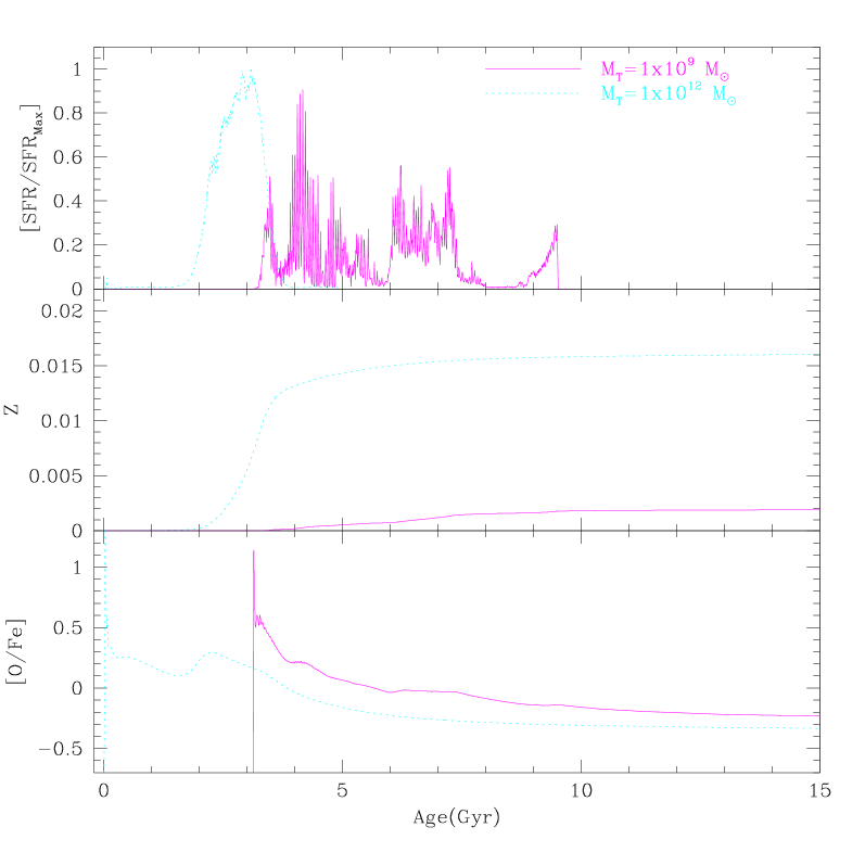
Figure 1: Bottom: the temporal variation of the abundance ratio [O/Fe] in models 3B and 6B-LD. Middle: the temporal variation of the metallicity in the same models. Top: the SFR of the same models normalized to the peak value SFR_Max.

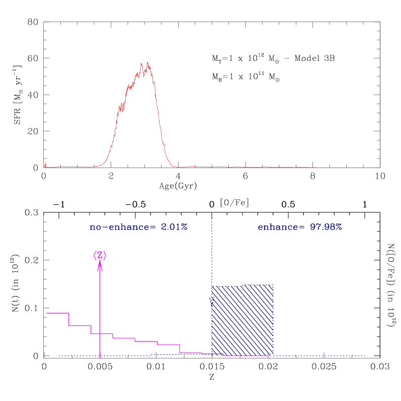
Figure 2: The top panel shows the SF history of the 3B model with total mass $\rm M_{T}=10^{12}M_{\odot}$ and baryonic mass $\rm M_{B}=10^{11}M_{\odot}$. The SFR is in $M_{\odot}$/yr and time is in Gyr. The bottom panel gives the cumulative number of living stars per bin of metallicity Z (solid line and bottom x-axis) and per bin of [O/Fe] (dotted line and top X-axis). The shaded zone shows the region populated by the stars with [O/Fe]$>$0, the $\alpha$-enhanced component. The percentage of star numbers with [O/Fe]$>$0 is about 98%, whereas that with [O/Fe]$<$0 is 2 %.

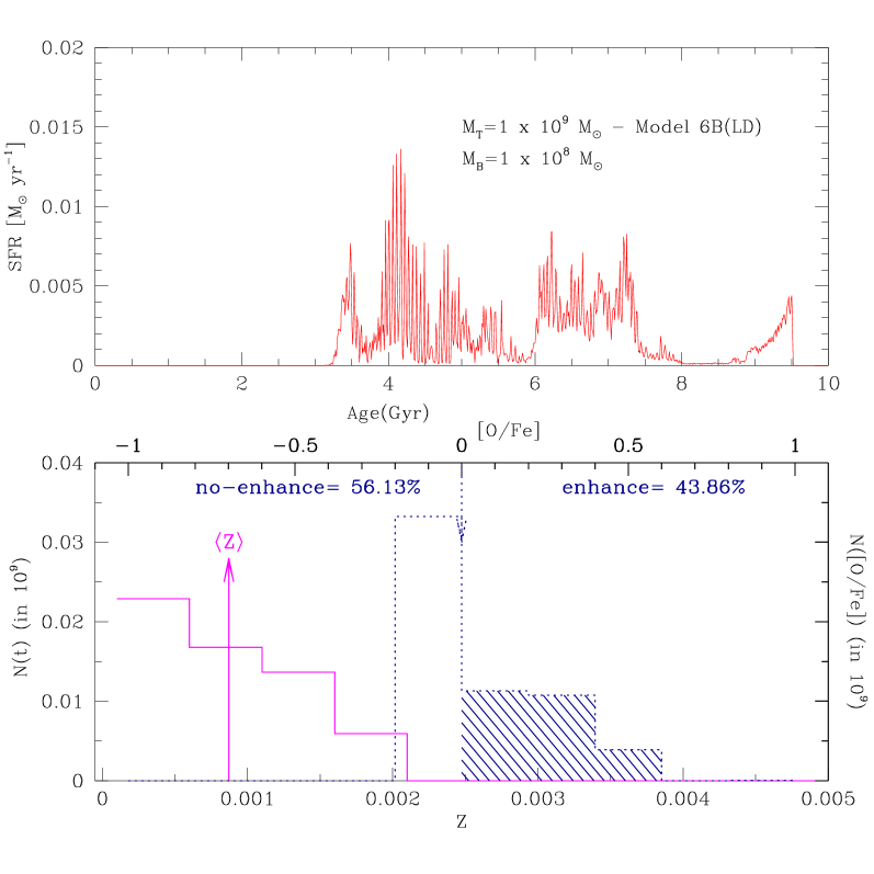
Figure 3: The same of Fig. 2 but for the 6B-LD galaxy, the object with the lowest initial density and the longest duration of stellar activity. The total mass is $\rm M_{T}=10^{9}M_{\odot}$, whereas the baryonic mass is $\rm M_{T}=10^{9}M_{\odot}$. The percentage of $\alpha$-enhanced stars is now 44%

3.3 Chemical abundances and abundance ratios

The chemical evolution of all the models presented in Table 1 has been followed and the results of interest here are best represented by the series of Figs. 1 through 3.

In Fig. 1 we show the time variation of the SFR (top panel), the metallicity Z (mid panel), and the abundance ratio [O/Fe] (bottom panel) for the models 3B with $\rm M_{T}=10^{9}M_{\odot}$ and 6B-LD with $\rm M_{T}=10^{9}M_{\odot}$ as indicated. As expected, during the period of stellar activity, the metallicity increases, whereas when star formation is over the metallicity remains either constant or slightly decreases by dilution with gas ejected by old stars of low metal content. Looking at the time variation of the abundance ratio [O/Fe] – a measure of the $\alpha$-enhancement level – we note that

(i) Within the first 0.1 Gyr the abundance ratios are lowered to values comparable to the mean ones under the contamination by the first Type Ia supernovae.

(ii) Even a small amount of stellar activity changes the initial abundance ratios to much lower values.

(iii) Subsequent star formation does not alter the abundance ratios significantly. See for instance the case of the $\rm 10^{12}\,M_{\odot}$ galaxy in which the prominent burst occurring from 2 to 3.5 Gyr changes (increases) the [O/Fe] ratio by less than $\rm\Delta[O/Fe]$=0.2 (less than a factor of two).

(iv) Once star formation has ceased, almost immediately the effect of Type II supernovae stops and that by Type Ia takes over first rapidly and later slowly decreasing [O/Fe] towards the solar value or below this.

In order to answer the question whether or not the present-day stellar content of these galaxies would appear to be enhanced in $\alpha$-elements, we look at the cumulative distribution of the number of living stars in different bins of [O/Fe]. From an operational point of view a galaxy will be considered dominated by an $\alpha$-enhanced stellar content if $\rm\sum N([O/Fe]>0)/N_{T}>0.5$, where $\rm\sum N([O/Fe])$ is the number of stars in bins with [O/Fe]$>$0 and $\rm N_{T}$ is their total number. The opposite if $\rm\sum N([O/Fe]<0)/N_{T}<0.5$. The situation for the two galaxies under examination is shown in Fig. 2 ($\rm 10^{12}\,M_{\odot}$) and Fig. 3 ($\rm 10^{9}\,M_{\odot}$).

The massive galaxy (Fig. 2), characterized by a rather short ($\sim 2.5$ Gyr) and prominent burst of star formation activity has about 98% of its stellar content in bins with with [O/Fe]$>0$. Whereas the low mass, low initial density galaxy (Fig. 3), whose star formation stretched over long periods of time in several recurrent episodes, has the majority of stars in bins with [O/Fe]$<0$ ($\sim$44%).

The percentage of stars with $\rm N([O/Fe])/N_{T}>0.5$ are listed in column (9) of Table 1. Finally, in columns (3) and (4) and of Table 4 to better described below we list the maximum, $\rm Z_{Max}$, and the mean metallicity, $\rm\langle Z\rangle$, of our model galaxies.

Figure 4: Schematic SFRs of our simulations. See the text for more details.

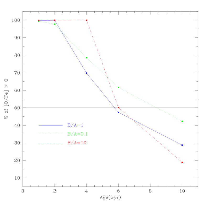
Figure 5: Degree of enhancement in models with different shape and duration of the SFR. The dotted line is for B/A=0.1, the solid line for B/A=1, and the dashed line for B/A=10. See the text for more details

4 What does determine the enhancement of $\alpha$-elements?

The entries of Table 1 show that the percentage of stars with [O/Fe]$>$0 decreases with the total duration of the star formation activity $\rm\Delta T_{SF}$. However all models but for the case 6B-LD have percentages of $\alpha$-enhanced stars higher than 50%. In order to understand under which circumstances (shape of the SFR and $\rm\Delta T_{SF}$) a galaxy would build a stellar population with a percentage of $\alpha$-enhanced stars less than 50%, we have performed the following experiment. We have taken one of the most unfavorable cases, i.e. a typical galaxy with $\rm M_{T}=10^{12}\,M_{\odot}$ and hence $\rm M_{B}=10^{11}\,M_{\odot}$, imposed that the same amount of mass in stars is build up at the end of the star forming activity, and varied both the shape and duration, $\rm\Delta T_{SF}$ of the SFR.

We adopt a simple analytical expression for the SFR as illustrated in Fig. 4. This is idealized to a trapezium of sides A, B and $\rm\Delta T_{SF}$. By varying the ratio B/A, the shape of the SFR changes from case (1) in Fig. 4 with B/A$<<$ 1 (SFR peaked in the past), to a constant SFR with B/A=1 of case (2) in Fig. 4, and finally to case (3) in Fig. 4 (SFR peaked toward the present). The total area of the trapezium (rectangle) yields the total mass $\rm M_{s}$ in stars build up in the galaxy. The galaxy under consideration has a total mass in stars of about $\rm 6.4\times 10^{10}\,M_{\odot}$.

The following relationship holds between $\rm M_{s}$ and SFR

$$\rm M_{s}=0.5\times A\big{[}1+{B\over A}\big{]}\times\Delta T_{SF}$$ (4)

from which we may easily derive an analytical expression for the SFR to be plugged into the chemical code. We have explored the following combinations of the parameters B/A=0.1, 1.0, and 10 and $\rm\Delta T_{SF}$=1, 2, 4, 6 and 10 Gyr. The results are displayed in Fig. 5, which plots the present-day percentage of $\alpha$-enhanced stars as a function of $\rm\Delta T_{SF}$ and the ratio B/A (the dotted line for B/A=0.1, the solid line for B/A=1, and the dashed line for B/A=10). It is soon evident that $\rm\Delta T_{SF}$ is the dominant parameter, whereas the ratio B/A plays a marginal role. With the prescription for Type Ia supernovae we have adopted, to fall below the border line of 50%, $\rm\Delta T_{SF}$ should be longer than about 6 Gyr and the stellar activity should be uniformly diluted. This is indeed the case of 6B-LD model which finds confirmation by the present analysis. A counter-example is the case of the 7B model with $\rm M_{T}=10^{8}\,M_{\odot}$ whose $\rm\Delta T_{SF}\simeq$6.5 Gyr but the SFR is mostly confined between 2 to 4 Gyr with the peak at about 3 Gyr. The reason for that is the initial density which is slightly higher than that of case 6B-LD (see Table 1 and Chiosi & Carraro (2001) for all details). The total duration of the SFR and not its shape drives the level of enhancement.

5 Mean narrow band indices for galaxies

In this section we evaluate the narrow band indices for our model galaxies in order to check how far they can go in reproducing important relationships such as the $\rm Mg_{2}$ versus $\sigma$ (Burstein et al. 1988) and the $\rm H_{\beta}$ versus $\rm Mg_{2}$ and/or $\rm MgFe$, see for instance González (1993); Trager et al. (2000a, b).

In presence of enhancement in $\alpha$-elements one has to modify the relationship between the total metallicity $Z$ and the iron content [Fe/H] by suitably defining the enhancement factor $\Gamma$. For more details see Tantalo (1998) and Tantalo & Chiosi (2002).

Let us split the metallicity $Z$ in the sum of two terms

$$\rm Z=\sum_{j}X_{j}+X_{Fe}$$ (5)

where $\rm X_{j}$ are the abundances by mass of all heavy elements but Fe, and $\rm X_{Fe}$ is the same for Fe. Recasting eq.(5) as

$$\rm Z=\frac{X_{Fe}}{X_{H}}X_{H}\left[1+\frac{\sum_{j}X_{j}}{X_{Fe}}\right]$$ (6)

and normalizing it to the solar values we get

$$\rm\left(\frac{Z}{Z_{\odot}}\right)=\left(\frac{X_{Fe}}{X_{H}}\right)\left(\frac{X_{H}}{X_{Fe}}\right)_{\odot}\left(\frac{X_{H}}{X_{H,\odot}}\right)\frac{\left[1+\frac{\sum_{j}X_{j}}{X_{Fe}}\right]}{\left[1+\frac{\sum_{j}X_{j}}{X_{Fe}}\right]_{\odot}}$$ (7)

from which we finally obtain

$$\rm\left[\frac{Fe}{H}\right]=\lg{\left(\frac{Z}{\mbox{${\rm Z_{\odot}}$}}\right)}-\lg{\left(\frac{X}{\mbox{${\rm X_{\odot}}$}}\right)}-\Gamma$$ (8)

which provides also the definition of $\Gamma$. Obviously for solar metallicity $\rm Z_{\odot}$ and solar-scaled mixture ($\Gamma=0.0$) eq.(8) yields [Fe/H]$=0.0$. In general, when dealing with enhanced chemical mixtures, it suffices to determine $\Gamma$ according to the degree of enhancement and simply re-scale the zero-point for the iron content of the Sun, i.e [Fe/H]=-$\Gamma$). Remarkably, enhancing $\alpha$-elements simply reduces to decreasing [Fe/H].

Table 2 lists the initial chemical composition and the iron abundances corresponding to $\Gamma$=0 and $\Gamma$=0.356, the same as the stellar models and isochrones of Salasnich et al. (2000) on which our indices are ultimately based.

Table 2: Real [Fe/H] for solar-scaled and $\alpha$-enhanced isochrones as a function of the initial chemical composition [X,Y,Z].

			$\Gamma=0.0$	$\Gamma=0.356$
Z	Y	X	[Fe/H]	[Fe/H]
0.008	0.248	0.7440	–0.3972	–0.7529
0.019	0.273	0.7080	0.0000	–0.3557
0.040	0.320	0.6400	0.3672	0.0115
0.070	0.338	0.5430	0.6824	0.3267

Once $\Gamma$ is known for the stellar population under consideration, to proceed further we need a calibration expressing the indices as a function of it. To this purpose we make use of the calibration by Borges et al. (1995) for ${\rm Mg_{2}}$  in which the effect of enhancement is considered. According to Borges et al. (1995), the index ${\rm Mg_{2}}$ of a “star” with enhanced content of Mg is given by the relation

$$\rm{\ln}{Mg_{2}}=-9.037+5.795\frac{5040}{T_{eff}}+0.398\log{g}+\leavevmode\nobreak\ \leavevmode\nobreak\ \leavevmode\nobreak\ \leavevmode\nobreak\ \leavevmode\nobreak\ \leavevmode\nobreak\ \leavevmode\nobreak\ \leavevmode\nobreak\$$

$$\rm\leavevmode\nobreak\ \leavevmode\nobreak\ \leavevmode\nobreak\ \leavevmode\nobreak\ \leavevmode\nobreak\ \leavevmode\nobreak\ \leavevmode\nobreak\ \leavevmode\nobreak\ 0.389\left[\frac{Fe}{H}\right]-0.16\left[\frac{Fe}{H}\right]^{2}+0.981\left[\frac{Mg}{Fe}\right]$$ (9)

which holds for effective temperatures and gravities in the ranges $\rm 3800<T_{eff}<6500$ K and $\rm 0.7<\log{g}<4.5$. To make use of eq.(9), we need [Mg/Fe] as function of $\Gamma$. The correspondence between [Mg/Fe] and $\Gamma$ can be obtained in the following way: from the pattern of abundances by Anders & Grevesse (1989); Grevesse (1991) and Grevesse & Noels (1993) we get the approximated relation

$$\rm\Gamma\simeq 0.8\left[\frac{Mg}{Fe}\right]$$ (10)

According to which [Mg/Fe]=0.0 for $\Gamma$=0 (solar-scaled abundances), and [Mg/Fe]=0.444 for $\Gamma$=0.356.

For all remaining indices we use the Worthey et al. (1994) fitting functions in which the enhancement of $\alpha$-elements is taken into account only via the re-scaled value of [Fe/H] of eq.(8).

Table 3: Coefficients for the relation (11) and the calibration by Borges et al. (1995).

$I_{i}$	$a_{1,i}$	$a_{0,i}$	$b_{1,i}$	$b_{0,i}$	$c_{0,i}$	$\delta_{i}$
$\rm H_{\beta}$	–0.565 $\pm$ 0.134	–1.356 $\pm$ 0.228	–0.295 $\pm$ 0.140	–0.673 $\pm$ 0.029	0.205 $\pm$ 0.015	2.89
$\rm Mg_{2}$	0.089 $\pm$ 0.034	0.135 $\pm$ 0.056	–0.072 $\pm$ 0.027	0.165 $\pm$ 0.030	–0.093 $\pm$ 0.010	0.10
$\rm\langle Fe\rangle$	0.488 $\pm$ 0.132	0.845 $\pm$ 0.580	0.357 $\pm$ 0.113	1.725 $\pm$ 0.185	0.898 $\pm$ 0.026	2.18
$\rm Mg_{b}$	1.103 $\pm$ 0.234	1.676 $\pm$ 0.675	0.115 $\pm$ 0.298	2.011 $\pm$ 0.359	0.806 $\pm$ 0.066	2.09

Looking at the response of indices to variations of the age, $\rm\log(t)$ in Gyr, metallicity $\rm\log(Z/Z_{\odot})$, and degree of enhancement $\Gamma$ of SSPs, we derive the following analytical relationships,

$$\begin{array}[]{ll}\rm I_{i}=\left(a_{1,i}\Gamma+a_{0,i}\right)\log(t)\\ \leavevmode\nobreak\ \leavevmode\nobreak\ \leavevmode\nobreak\ \leavevmode\nobreak\ \leavevmode\nobreak\ \leavevmode\nobreak\ +\left(b_{1,i}\Gamma+b_{0,i}\right)\log{\left(\frac{Z}{Z_{\odot}}\right)}+c_{0,i}\Gamma+\delta_{i}\end{array}$$ (11)

where $\rm I_{i}$ for $i$=1 to 4 stand for the ${\rm H_{\beta}}$, ${\rm Mg_{2}}$, ${\rm\langle Fe\rangle}$ and ${\rm Mg_{b}}$, respectively. The coefficients are tabulated in Table 3 for the Borges et al. (1995) calibration. These analytical fits are accurate enough for the purposes of the present study.

Given these premises, we derive the indices for our model galaxies as follows:

(i) With the aid of the cumulative distributions of living stars per [O/Fe] bins (see the bottom panels of Figs. 3 and 2 and those for all remaining models not shown here for the sake of brevity), we estimate the mean value of [O/Fe] weighed on the number of stars per bin and consider it as an estimate of the enhancement factor $\Gamma$. This is found to weakly correlate with the velocity dispersion of the galaxy $\Gamma=0.072\,log\sigma+0.134$.

(ii) From the history of star formation (top panels of the same Figures.) we estimate the mean age $\rm T_{BS}$ of the bulk stars. To do so one has to convert the rest-frame ages of the galaxy models into an absolute age by means of a cosmological model of the Universe. To make things simple we adopt here the Freedman model with $\rm H_{0}$=50 km s^-1 Mpc^-1, $\rm q_{0}$=0 and red-shift of galaxy formation $\rm z_{for}=5$, which yield the maximum age for galaxies $\rm T_{G}$=16.5 Gyr. The age $\rm T_{BS}$ is therefore $\rm T_{BS}=T_{G}-T_{PSF}$, where $\rm T_{PSF}$ is the time at which the peak of star formation occurred. These quantities are listed in columns (5) and (6) of Table 4.

(iii) Finally, we make use of relations (11) to derive the indices $\rm H_{\beta}$, $\rm Mg_{2}$, $\rm\langle Fe\rangle$, and $\rm Mg_{b}$ for both the maximum and mean metallicity (age $\rm T_{BS}$ and $\Gamma$ are the same). The results are listed in Table 4.

Table 4: Theoretical indices for all the models under considerations. The calibration in use is by Borges et al. (1995).

Model	$\rm M_{T}$	$\rm Z_{Max}$	$\rm\langle Z\rangle$	$\Gamma$	$\rm T_{BS}$	$\rm H_{\beta}$	$\rm Mg_{2}$	$\rm\langle Fe\rangle$	$\rm Mg_{b}$	$\rm H_{\beta}$	$\rm Mg_{2}$	$\rm\langle Fe\rangle$	$\rm Mg_{b}$
						Maximum Z				Mean Z
1A	$1\times 10^{13}$	0.020	0.005	0.53	16.3	1.47	0.26	2.49	3.09	1.79	0.14	1.56	1.91
6A	$1\times 10^{9}$	0.004	0.002	0.66	16.3	1.89	0.11	1.18	1.33	2.08	0.02	0.57	0.54
1B	$5\times 10^{13}$	0.025	0.008	0.14	14.5	1.30	0.28	3.15	3.98	1.61	0.19	2.33	2.99
2B	$5\times 10^{12}$	0.018	0.007	0.27	13.0	1.51	0.24	2.69	3.36	1.75	0.17	2.02	2.55
3B	$1\times 10^{12}$	0.015	0.005	0.19	12.0	1.57	0.23	2.65	3.31	1.86	0.14	1.86	2.36
5B	$1\times 10^{10}$	0.006	0.003	0.15	11.0	1.85	0.15	2.01	2.54	2.03	0.10	1.53	1.97
6B-LD	$1\times 10^{9}$	0.001	0.002	0.05	6.0	2.69	0.01	0.59	0.75	2.47	0.04	1.14	1.39
6B	$1\times 10^{9}$	0.004	0.002	0.12	10.0	2.01	0.12	1.72	2.18	2.14	0.08	1.38	1.78
6B-HD	$1\times 10^{9}$	0.006	0.002	0.19	12.0	1.81	0.15	1.99	2.52	2.11	0.07	1.20	1.57
7B	$1\times 10^{8}$	0.003	0.001	0.18	8.0	2.22	0.08	1.37	1.68	2.51	0.01	0.58	0.73

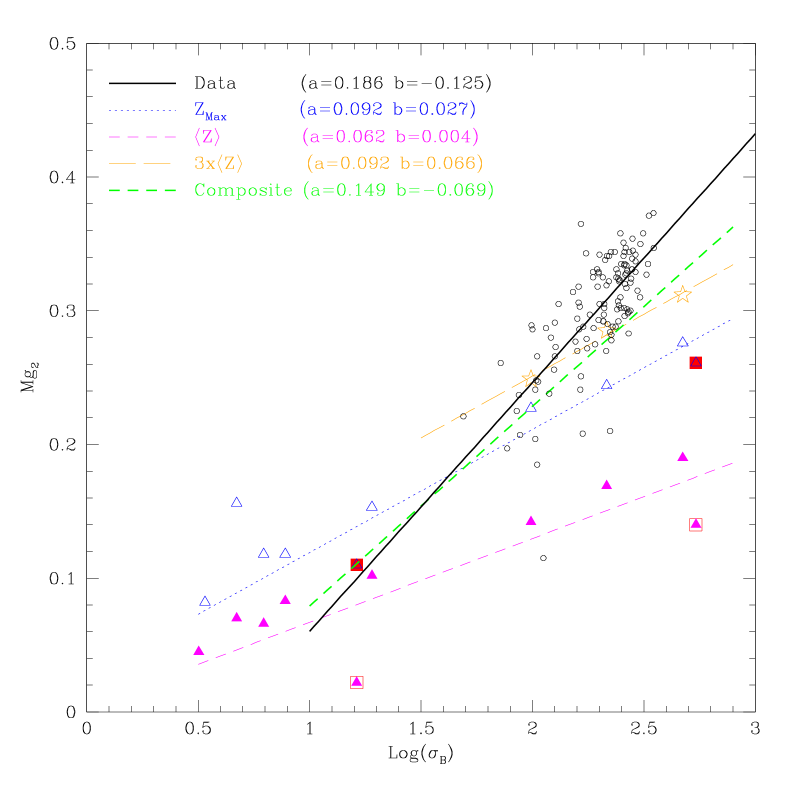
Figure 6: The $\rm Mg_{2}$ versus velocity dispersion $\sigma_{B}$. The small open circles are the observational data from Trager et al. (2000a, b) and the solid line is their least squares fit. The open and filled triangles are the theoretical models of type B listed in Table 4 for the maximum and mean metallicity, respectively. Their least square fits are shown by the dashed ($\rm Z_{Max}$) and dotted ($\rm\langle Z\rangle$) lines. The three empty stars show the same, however limited to the three most massive galaxies, but for a metallicity arbitrarily increased to $\rm 3\times\langle Z\rangle$. The thick dashed line shows the composite case in which the metallicity of the three most massive galaxies is $\rm 3\times\langle Z\rangle$ and that of the less massive ones is $\rm\langle Z\rangle$. The filled squares ($\rm Z_{Max}$) and boxed-filled triangles ($\rm langleZ\rangle$ show the case of models A.

The $\rm Mg_{2}$ vs $\sigma$ relation. This is shown in Fig. 6 and compared with the observational data by Trager et al. (2000a, b) for a sample of local EGs. The least squares fit of the observational data yields the relation $\rm Mg_{2}=0.186\,log\sigma-0.125$ (where $\sigma$ is in km s^-1). The theoretical results are plotted separately for each of the metallicities in use: the filled triangles are for $\rm\langle Z\rangle$ (a more realistic approximation of reality) and the open triangles are for $\rm Z_{Max}$. The least squares fit of the data yields $\rm Mg_{2}=0.063\,log\sigma+0.001$ for $\langle Z\rangle$ and $\rm Mg_{2}=0.094\,log\sigma+0.063$ for $Z_{Max}$. The slope is about half of what observed. Where is the source of disagreement? There are several candidates: (i) the velocity dispersion, (ii) the calibration in use, (iii) the set of parameters $\rm T_{BS}$, $\rm Z$ and $\Gamma$ assigned to the model galaxies. Limiting the discussion to the range of massive models for which data exist, we note:

(i) The velocity dispersion is not likely because it should be decreased by a factor of two and in any case the relation would simply horizontally shift without changing its slope.

(ii) The calibration is more uncertain, even though the one in use here allowing for the maximum effect. In this context one should, however, keep in mind that, contrary to what one may guess, increasing $\Gamma$ (higher enhancement) does not imply a stronger $\rm Mg_{2}$ because of the counter-reaction by [Fe/H].

(iii) Assuming that our velocity dispersions and calibration are correct, inspection of the weight of $T_{BS}$, $\Gamma$, and $\rm Z$ on building up the final result reveals that the metallicity dominates. The three empty stars show the effect of arbitrarily increasing $\rm\langle Z\rangle$ by a factor of 3, limited to the three most massive galaxies. This implies that the $\rm Mg_{2}$ vs $\sigma$ relation reflects the mass-metallicity relation, rather a sequence in the enhancement level.

Are the mean (and maximum) metallicity reasonable? Is there any plausible effect making a massive galaxy more efficient in building metals? With the IMF adopted here and in the dynamical models, the production of metals is scarcely efficient because of the low $\zeta$, Increasing this for all galaxies would simply shift vertically the $\rm Mg_{2}$ vs $\sigma$ relation. However, if $\rm\zeta$ increases with the galaxy mass (top-heavy IMF), theory and data could be reconciled. Although this possibility has often been advanced by several authors in different astrophysical contexts – see the arguments given by Chiosi et al. (1998) and Larson (1998) – further exploring the subject is beyond the scope of this paper. Suffice to conclude that dynamical models almost match the observational $\rm Mg_{2}$ vs $\sigma$ relation provided some fine tuning of the chemical yields per stellar generation is applied. Just for the sake of curiosity, we derive the relationship one would obtain by letting the mean metallicity to increase from the present values to $\rm 3\times\langle Z\rangle$ as the galaxy mass mass increases from $10^{9}$ to $\rm 5\times 10^{12}\,M_{\odot}$. We get $\rm Mg_{2}=0.149\,log\sigma-0.070$, which is about right.

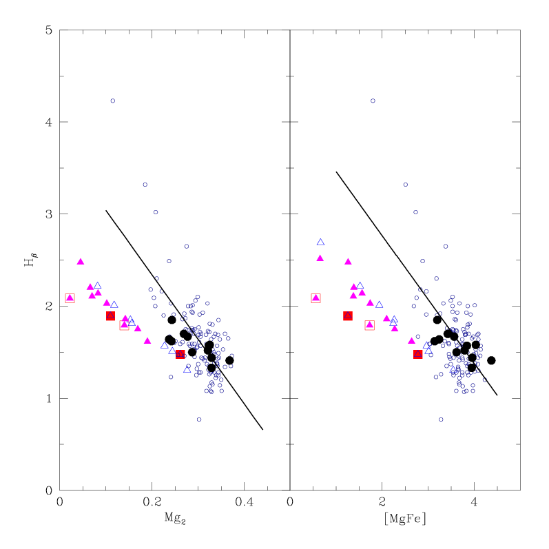
Figure 7: The $H_{\beta}$ versus $Mg_{2}$ and $MgFe$ planes. The meaning of the symbols is the same as in Fig. 6. We have also added the small sample of EGs in Fornax by Kuntschner (2000) (big filled circles). The line is the linear fit of all observational data.

The $\rm H_{\beta}$ versus $\rm Mg_{2}$ and $\rm MgFe$ planes. The index-index planes are customarily used to infer age and metallicity of early-type galaxies (González 1993; Bressan et al. 1996; Trager et al. 2000a, b; Kuntschner 2000, 2001). In Fig. 7 we present the $\rm H_{\beta}$ vs $\rm Mg_{2}$ and $\rm H_{\beta}$ vs $\rm MgFe$ planes left and right panels respectively, for our models, single stellar populations of similar metallicity, and observational data for a small sample of EGs in the Fornax cluster by Kuntschner (2000) and the wider sample of nearby galaxies by Trager et al. (2000a). The following remarks can be made:

(i) Our models lie on a strip which roughly correspond to that covered by SSP of different metallicity and age in the range say 15 to 8-10 Gyr. This expected because all models have terminated their star formation far in the past. Even the most extreme case has ceased star formation 6 Gyr ago.

(ii) Also in these planes we notice the same kind of difficulty encountered with the $\rm Mg_{2}$ vs $\sigma$ relation, i.e. our model galaxies do not make enough metals so that even the most massive ones only marginally reach the region crowed by the data. The same kind of arguments brought about to cure the $\rm Mg_{2}$ vs $\sigma$ relation apply here. Increasing the metal content of the model galaxies is less of a problem.

6 Concluding remarks

In this paper we have derived the present-day level of enhancement in $\alpha$-elements in the stellar content of the N-Body Tree-SPH models of EGs by Chiosi & Carraro (2001), cast light on the main cause of it, derived the mean spectral indices of the model galaxies, and compared them to the observations with particular attention to the $\rm Mg_{2}$-$\sigma$ relation and the $\rm H_{\beta}$ - $\rm Mg_{2}$–[MgFe] planes.

Combining the results of Chiosi & Carraro (2001) summarized in Section 3 and those obtained here the following remarks can be made:

(i) The star formation history of EGs depends on their total mass and initial density, i.e. the physical conditions of the environment in which they have formed. High-density systems, owing to their very early and short star forming activity would now appear as old galaxies, whose stellar content is enhanced in $\alpha$-elements. Low-density systems of high mass would resemble the previous ones, their stellar content should, however, span a broader range of ages. Most of the component stars should be enhanced in $\alpha$-elements but with a broader distribution of abundance ratios [$\alpha$/Fe]. At decreasing mass the star formation activity should become more diluted in time, the stellar populations should span wider and wider age ranges, and the level of enhancement should progressively tend to solar. The extreme case is reached with the low-mass, low-density systems which could undergo many episodes of star formation up to very recent times, thus resembling young objects with solar or sub-solar partitions of elements. It is worth recalling here that $\Gamma$ or equivalently [O/Fe] is found to weakly increase with the velocity dispersion (mass) of the galaxy.

(ii) The scenario sketched above is perhaps confirmed by the many observational studies based on different kinds of diagnostic. For instance Kuntschner & Davies (1998); Kuntschner (2000, 2001) studying early-type galaxies in the Fornax cluster find the EGs to be coeval and to have metallicities varying from solar to three times solar, and the ratio [Mg/Fe] –inferred from the indices $\rm Mg_{2}$ and Fe3– to weakly correlate with the velocity dispersion. In contrast the data for nearby field galaxies by González (1993); Bressan et al. (1996), and Trager et al. (2000a, b), seem to indicate a much broad range of ages as perhaps compatible with our model galaxies of low initial density. Finally, we call attention on the recent result by Poggianti et al. (2001) for dwarf galaxies confirming the suggestion made by Bressan et al. (1996) and Trager et al. (2000a, b) of a recent star formation in these systems.

(iii) The $\rm Mg_{2}$ vs $\sigma$ relation mainly reflects the metallicity-$\sigma$-mass sequence rather than enhancement in $\alpha$-elements and/or age.

(iv) Although the dynamical models and companion chemical models we have discussed do not fully match the high metallicities inferred from other diagnostics and some improvement is required, they however seem to offer a coherent scenario accounting for many observed properties of EGs, thus perhaps indicating that we are on the right track.