Cosmological Parameters from Redshift-Space Correlations

Abstract

We estimate how clustering in large-scale redshift surveys can constrain various cosmological parameters. Depth and sky coverage of modern redshift surveys are greater than ever, opening new possibilities for statistical analysis. We have constructed a novel maximum likelihood technique applicable to deep redshift surveys of wide sky coverage by taking into account the effects of both curvature and linear velocity distortions. The Fisher information matrix is evaluated numerically to show the bounds derived from a given redshift sample. We find that intermediate-redshift galaxies, such as the Luminous Red Galaxies (LRGs) in the Sloan Digital Sky Survey, can constrain cosmological parameters, including the cosmological constant, unexpectedly well. The importance of the dense as well as deep sampling in designing redshift surveys is emphasized.

1 Introduction

Recently, independent cosmological observations have turned out to be consistent with a canonical model of the structure formation based on the assumption that the main ingredients of our universe are the cold dark matter (CDM), and the dark energy component such as a cosmological constant. Introducing the unknown dark matter and the peculiar dark energy could have been thought of as somewhat artificial at the time when observations were not constraining enough, now this model has become more and more convincing with remarkable observational support.

To make a cosmological model truly convincing, it is important to make sure that any possible observations are consistent with that model. This can be accomplished by determining cosmological parameters as precisely as possible from each observation, and then comparing the results with one another. So far the individual observations were only able to constrain the parameters into some region in a multi-dimensional parameter space. Therefore, it is quite common to combine different observations to obtain the tight constraint on the parameters. A striking example is a combination of fluctuations in cosmic microwave background (de Bernardis et al., 2000) and a Hubble diagram of supernova Ia (Riess et al., 1998; Perlmutter et al., 1999) which is considered to be the prominent evidence of the current canonical model.

However, one can test the consistency of the theory only when each observation can independently constrain the parameters in a sufficiently small region. In this paper, we explore the capabilities of redshift surveys in this respect. In redshift surveys, there are several degrees of freedom in planning survey strategies: the area and the depth of a survey, and the choice of specific targets for the spectroscopic measurements. Each of these affects the analysis in a different and complex fashion. Thus, it is important to estimate the impact of a given strategy on the cosmological analysis of the data.

In this paper, we apply our considerations to the Sloan Digital Sky Survey (SDSS, York et al., 2000). It is not only the largest ongoing redshift survey, but it also contains three different types of spectroscopic targets within the same area of the sky that can be used to infer cosmological information.

In deep, wide redshift surveys like SDSS, the apparent clustering properties in observable redshift space are complicated because of the redshift-evolution and redshift-distortion effects. In linear regime, with a standard initial Gaussian density field, the correlation function $\xi(r)$ or the power spectrum $P(k)$ completely characterizes the statistical property of the density field. Spatial homogeneity and isotropy in real space guarantees these to be one-dimensional functions of the scale, $r$ or $k$. So it is usual to estimate the real-space power spectrum with certain correction methods or ansatz from observed redshift-space data, in order to compare with the theoretical prediction of various cosmological models (e.g., Davis & Peebles, 1983; Feldman, Kaiser & Peacock, 1994).

However, the redshift-evolution and redshift-distortion also have invaluable information on cosmology. The redshift-evolution of the density fluctuations depends on the growth factor which is a function of the density parameter $\Omega_{\rm M}$ and the normalized cosmological constant parameter $\Omega_{\rm\Lambda}$. It is also a function of the galaxy bias $b$ which contains the information on the unknown galaxy formation process. The redshift-distortion depends on the density-velocity relation which is a function of $\Omega_{\rm M}^{0.6}/b$ (Kaiser, 1987), and also on $\Omega_{\rm M}$ and $\Omega_{\rm\Lambda}$ through geometrical distortions (Alcock & Paczyński, 1979; Ballinger, Peacock & Heavens, 1996; Matsubara & Suto, 1996).

When our main purpose is not only determining the power spectrum of initial fluctuations, but also constraining above parameters, it is desirable to directly analyze the data to obtain cosmological information without any intermediate statistical quantities like the power spectrum. Since the apparent clustering in redshift space is quite different from that in real space, we can take advantage of the maximum-likelihood method to directly constrain cosmological models from the apparent clustering data in redshift space.

In our previous work (Matsubara & Szalay, 2001), we focused on how near-future redshift surveys can constrain the cosmological constant by the maximum-likelihood method. Since the redshift surveys become larger and larger, even the multi-dimensional parameter space can be constrained by redshift surveys alone. Combining with other cosmological observations like the cosmic microwave background fluctuations, Hubble diagram of the type Ia supernova, and so on, one can constrain the parameters more accurately. However, independent observational constraints can serve as a consistency check of the fundamental cosmological model. In this respect, we investigate how one can constrain the multi-dimensional parameter space of the standard CDM model with cosmological constant from redshift surveys, extending our previous work.

2 Maximum-likelihood Method for the Apparent Redshift-space Clustering

In maximum-likelihood methods, we directly deal with the density fluctuations in redshift space. In order to do this, first we place smoothing cells in redshift space and consider the number of objects $n_{i}$ in each cell $i$. Each count represents the smoothed density field contaminated by shot noise. For given mean number densities, $\bar{n}_{i}=\langle n_{i}\rangle$, the density fluctuations $a_{i}=n_{i}/\bar{n}_{i}-1$ are the fundamental quantities to be analyzed. In the following, the most important statistical quantity is the correlation matrix, $C_{ij}=\langle a_{i}a_{j}\rangle$. This matrix is related to a continuous two-point correlation function in redshift space $\xi({\mbox{\boldmath$s$}},{\mbox{\boldmath$s$}}^{\prime})=\langle\delta({\mbox{\boldmath$s$}})\delta({\mbox{\boldmath$s$}}^{\prime})\rangle$, where $\delta({\mbox{\boldmath$s$}})$ is the underlying continuous density contrast which survey objects trace. The relation between the correlation matrix and the correlation function is given by

$$C_{ij}=\int d^{3}s\,d^{3}s^{\prime}\,W^{\rm(s)}({\mbox{\boldmath$s$}}_{i}-{\mbox{\boldmath$s$}})W^{\rm(s)}({\mbox{\boldmath$s$}}_{j}-{\mbox{\boldmath$s$}}^{\prime})\,\xi({\mbox{\boldmath$s$}},{\mbox{\boldmath$s$}}^{\prime})+\int d^{3}s\,\frac{W^{\rm(s)}({\mbox{\boldmath$s$}}_{i}-{\mbox{\boldmath$s$}})W^{\rm(s)}({\mbox{\boldmath$s$}}_{j}-{\mbox{\boldmath$s$}})}{\bar{n}({\mbox{\boldmath$s$}})},$$ (2.1)

where $W^{\rm(s)}({\mbox{\boldmath$s$}})$ is the smoothing kernel in redshift space, normalized as $\int d^{3}sW^{\rm(s)}({\mbox{\boldmath$s$}})=1$ and $\bar{n}({\mbox{\boldmath$s$}})$ is the mean number density. The last term represents contribution from the shot noise effect. In linear regime, the two-point correlation function in redshift space is analytically given, including high redshift effect.

Although the general form is fairly complicated (Matsubara, 2000), the distant-observer approximation (Kaiser, 1987; Matsubara & Suto, 1996), which is applicable in many cases, simplify the analysis below. The corresponding formula (Matsubara & Suto, 1996; Matsubara, 2000) is given by

$$\xi({\mbox{\boldmath$s$}}_{1},{\mbox{\boldmath$s$}}_{2})=b(z_{1})b(z_{2})D(z_{1})D(z_{2})\int\frac{d^{3}k}{(2\pi)^{3}}e^{i{\mbox{\scriptsize\boldmath$k$}}\cdot({\mbox{\scriptsize\boldmath$x$}}_{1}-{\mbox{\scriptsize\boldmath$x$}}_{2})}\left[1+\beta(z_{1})\frac{{k_{\parallel}}^{2}}{k^{2}}\right]\left[1+\beta(z_{2})\frac{{k_{\parallel}}^{2}}{k^{2}}\right]P(k),$$ (2.2)

where $z_{1}$ and $z_{2}$ are the redshifts of the two points, $k_{\parallel}$ is the line-of-sight component of the wave number, $P(k)$ is the linear mass power spectrum at $z=0$, $D(z)$ is the linear growth rate normalized as $D(0)=1$, $b(z)$ is the bias factor at redshift $z$, and $\beta(z)$ is the redshift distortion parameter, which is accurately fitted by the redshift-dependent mass density parameter $\Omega_{\rm M}(z)$ and normalized cosmological constant $\Omega_{\rm\Lambda}$ as $\beta(z)\simeq\{\Omega_{\rm M}^{4/7}(z)+\Omega_{\rm\Lambda}(z)[1+\Omega_{\rm M}(z)/2]/70\}/b(z)$ (Lahav et al., 1991; Lightman & Schechter, 1990). The vectors ${\mbox{\boldmath$x$}}_{1}$ and ${\mbox{\boldmath$x$}}_{2}$ are the comoving positions of the two points which are labeled by ${\mbox{\boldmath$s$}}_{1}$ and ${\mbox{\boldmath$s$}}_{2}$ in redshift space (see Matsubara & Suto, 1996).

Except for the nearby universe, the comoving distance is not proportional to the redshift so that the smoothing kernel $W^{\rm(s)}$ in redshift space is distorted along the line of sight. In a distant-observer regime, a line-of-sight component $s_{\parallel}$ and a transverse component $s_{\perp}$ of redshift-space separation $s$ are given by

$$s_{\parallel}=H(z)x_{\parallel},\qquad s_{\perp}=\frac{z}{d_{A}(z)}x_{\perp},$$ (2.3)

where $x_{\parallel}$ and $x_{\perp}$ are corresponding line-of-sight and transverse components of real-space separation, respectively, and $z$ is the mean redshift. We have chosen the unit system $H_{0}=1$ here for simplicity. This unit system simplifies the equations in this section. We mention that another unit system for length is introduced in §4 for a practical reason which is explained there. In the above transform, the redshift-dependent Hubble’s parameter and the comoving angular diameter distance are explicitly given by

$$H(z)=\sqrt{\Omega_{\rm M}(1+z)^{3}+(1-\Omega_{\rm M}-\Omega_{\rm\Lambda})(1+z)^{2}+\Omega_{\rm\Lambda}},$$ (2.4)

$$d_{A}(z)=\left\{\begin{array}[]{ll}\displaystyle(-K)^{-1/2}\sinh\left[(-K)^{1/2}\chi(z)\right]&(K<0),\\ \displaystyle\chi(z)&(K=0),\\ \displaystyle K^{-1/2}\sin\left[K^{1/2}\chi(z)\right]&(K>0),\end{array}\right.$$ (2.8)

where

$$K=1-\Omega_{\rm M}-\Omega_{\rm\Lambda},\qquad\chi(z)=\int_{0}^{z}\frac{dz^{\prime}}{H(z^{\prime})},$$ (2.9)

are the curvature of the universe and comoving distance to the redshift $z$. Thus, the transform from the comoving space to the redshift space is the function of $\Omega_{\rm M}$ and $\Omega_{\rm\Lambda}$

As a result of the anisotropic transform of equation (2.3), the spherical kernel in redshift space, for example, ends up with oscillating two-dimensional numerical integration (Matsubara & Szalay, 2001) in evaluating the correlation matrix $C_{ij}$. Unfortunately, such numerical integration increases CPU time and decreases accuracy. This is crucial for the analysis of the real data, because the position of kernels can hardly be regular so that one has to calculate the correlation matrix pair by pair. The shape of the kernel is not important for largely separated pairs, but it affects nearby and identical pairs.

Although one can not exactly know what is the distortion unless the parameters $\Omega_{\rm M}$ and $\Omega_{\rm\Lambda}$ are fixed, it turns out to be a good approximation to set an approximate spherical kernel in real space with approximate values of these parameters. In fact, we found that the latter approximation is better than doing the exact numerical integration which inevitably has integration errors. When the parameters $\Omega_{\rm M}$ and $\Omega_{\rm\Lambda}$ should also be determined in real analyses, one can iterate the analysis to use better estimates for those parameters, but approximate values are good enough. Thus, suppose that we can approximately set a spherical kernel in real space, so that we have $W^{\rm(s)}({\mbox{\boldmath$s$}})=J^{-1}W_{R}(|{\mbox{\boldmath$x$}}|)$, where $J=\partial({\mbox{\boldmath$s$}})/\partial({\mbox{\boldmath$x$}})$ is the Jacobian from $x$-space to $s$-space, and $R$ is the (effective) smoothing radius. In the distant-observer approximation, $J(z)=z^{2}H(z)/{d_{A}}^{2}(z)$.

This approximation dramatically simplifies the evaluation of the correlation matrix. In fact, when the kernels are spherical in real space, at least approximately, equations (2.1) and (2.2) give

$$C_{ij}=b_{i}b_{j}D_{i}D_{j}\int\frac{d^{3}k}{(2\pi)^{3}}e^{i{\mbox{\scriptsize\boldmath$k$}}\cdot({\mbox{\scriptsize\boldmath$x$}}_{i}-{\mbox{\scriptsize\boldmath$x$}}_{j})}\left[1+\beta_{i}\frac{{k_{\parallel}}^{2}}{k^{2}}\right]\left[1+\beta_{j}\frac{{k_{\parallel}}^{2}}{k^{2}}\right]W^{2}(kR)P(k)$$

$$\qquad\qquad\qquad+\,\frac{1}{\sqrt{{J_{i}J_{j}\bar{n}_{i}\bar{n}_{j}}}}\int\frac{d^{3}k}{(2\pi)^{3}}e^{i{\mbox{\scriptsize\boldmath$k$}}\cdot({\mbox{\scriptsize\boldmath$x$}}_{i}-{\mbox{\scriptsize\boldmath$x$}}_{j})}W^{2}(kR),$$ (2.10)

where $b_{i}=b(z_{i})$, $D_{i}=D(z_{i})$, $J(z_{i})=J_{i}$, etc., and $W(kR)$ is the three-dimensional Fourier transform of the spherical kernel $W_{R}(|{\mbox{\boldmath$x$}}|)$. In our notation, $\bar{n}_{i}$ is the mean number density in redshift space so that $J_{i}\bar{n}_{i}$ is the mean number density in real space. We assume that the variation of the selection function within a kernel is negligible. The above equation means that the distant-observer redshift-distortion is commutable with spherical smoothing in real space, comparing with equation (2.2) besides shot-noise term. Angular integration of the first term can be analytically performed (see Hamilton, 1992; Matsubara & Suto, 1996; Matsubara, 2000), resulting in

$$C_{ij}=b_{i}b_{j}D_{i}D_{j}\left\{\left[1+\frac{1}{3}(\beta_{i}+\beta_{j})+\frac{1}{5}\beta_{i}\beta_{j}\right]P_{0}(\mu_{ij})\xi_{0}(x_{ij},R)\right.$$

$$\quad\qquad\qquad\qquad-\,\left.\left[\frac{2}{3}(\beta_{i}+\beta_{j})+\frac{4}{7}\beta_{i}\beta_{j}\right]P_{2}(\mu_{ij})\xi_{2}(x_{ij},R)+\frac{8}{35}\beta_{i}\beta_{j}P_{4}(\mu_{ij})\xi_{4}(x_{ij},R)\right\}$$

$$\qquad\qquad\qquad+\,\frac{1}{\sqrt{{J_{i}J_{j}\bar{n}_{i}\bar{n}_{j}}}}\int\frac{k^{2}dk}{2\pi^{2}}j_{0}(kx_{ij})W^{2}(kR),$$ (2.11)

where $\beta_{i}=\beta(z_{i}),\beta_{j}=\beta(z_{j})$, $x_{ij}=|{\mbox{\boldmath$x$}}_{i}-{\mbox{\boldmath$x$}}_{j}|$ is the comoving separation between the centers of the kernels, $\mu_{ij}=x_{ij\parallel}/x_{ij}$ is the direction-cosine of the separation $x_{ij}$ relative to the line of sight, $j_{l}$ is the spherical Bessel function, and $P_{l}(\mu)$ is the Legendre polynomial. We also define the quantity,

$$\xi_{l}(x,R)=\int_{0}^{\infty}\frac{k^{2}dk}{2\pi^{2}}j_{l}(kx)W^{2}(kR)P(k).$$ (2.12)

We need to numerically integrate the equation (2.12). Once we make a table of the integrated results for various $x$ and $R$ of interest, we can use this table to interpolate $\xi_{l}$, which makes the evaluation of the correlation matrix $C_{ij}$ a really fast operation. This method is very effective because the number of elements of a correlation matrix is the square of the number of cell sites $(N_{\rm cell})^{2}$, where $N_{\rm cell}\sim 1,000$–$10,000$, or more. We tried exact 2-dimensional integrations for identical and nearby cell-pairs, and found that they agree with the above approximation within the integration errors, even though the assumed $\Omega_{\rm M}$ and $\Omega_{\rm\Lambda}$ are different from the true values by a factor of about 0.5.

The shot noise term is diagonal when the kernels do not overlap each other, as one can see from the equation (2.1). Using a finite-volume kernel without any overlapping region, the last term of equation (2.1) or (2.11) is given by

$$\frac{\delta_{ij}}{\bar{n}_{i}}\int d^{3}s\left[W^{\rm(s)}({\mbox{\boldmath$s$}})\right]^{2}=\frac{\delta_{ij}}{J_{i}\bar{n}_{i}}\int\frac{k^{2}dk}{2\pi^{2}}W^{2}(kR).$$ (2.13)

The top-hat kernel, $W_{R}(x)=3\Theta(R-x)/(4\pi R^{3})$, where $\Theta$ is the step function, is the most popular example of the finite-volume kernel, in which case the above shot noise term simply reduces to $\delta_{ij}/\bar{N}_{i}$, where $\bar{N}_{i}=4\pi R^{3}J_{i}\bar{n}_{i}/3$ is the expected mean number count in a cell.

Although we only use the top-hat kernel in this paper, it is also useful to consider another possibility as digression, since this fast numerical approximations will also be used in the analysis of the real data. The top-hat kernel is not a smooth function, thus it is sometimes desirable to have an smoother kernel. An example of the smoother, yet finite-volume kernels is the Epanechnikov kernel, which is defined by $W_{R}(x)=15(1-x^{2}/R^{2})\Theta(R-x)/(8\pi R^{3})$. While the top-hat kernel is discontinuous on the edge $x=R$, the Epanechnikov kernel is continuous. The derivative is still discontinuous on the edge. One can also use the $m$-weight Epanechnikov kernel defined by

$$K_{m}(x;R)=\frac{(2m+3)!!}{m!\ 2^{m+2}\pi R^{3}}\left(1-\frac{x^{2}}{R^{2}}\right)^{m}\Theta(R-x).$$ (2.14)

The top-hat kernel and the Epanechnikov kernel are the special cases of this general Epanechnikov kernel with $m=0$ and $m=1$, respectively. The $(m-1)$-derivative of the $m$-weight Epanechnikov kernel is continuous on the edge. The larger the rank in the general Epanechnikov kernel is, the more regular it is on the edge. However, the effective volume of the kernel is smaller for a larger-weight kernel when a smoothing length $R$ is fixed. Taking limits $m\rightarrow\infty,R\rightarrow\infty$ with $m^{-1/2}R$ fixed, one can show that the higher-weight Epanechnikov kernel reduces to a Gaussian kernel with a variance $R/\sqrt{2m}$. The Fourier window function for the $m$-weight Epanechnikov kernel has a simple form,

$$W_{m}(kR)\equiv\int_{0}^{\infty}d^{3}xe^{-i{\mbox{\scriptsize\boldmath$k$}}\cdot{\mbox{\scriptsize\boldmath$x$}}}K_{m}(x;R)=\frac{(2m+3)!!\ j_{m+1}(kR)}{(kR)^{m+1}}.$$ (2.15)

The larger the rank $m$ is, the faster the window function drops off with the wavenumber $k$, which reflects the smoothness on the edge of the kernel. It is desirable to have a degree of freedom to choose an appropriate rank $m$, because one can optimize the analysis depending on the nature of an individual data set.

The observational data is the set of discrete density fluctuations $a_{i}$. The cosmological models are characterized by a given set of parameters $(\theta_{\alpha})$. Besides $\Omega_{\rm M}$, $\Omega_{\rm\Lambda}$, and $b$, which is explicitly appeared in the expression of the correlation matrix, the power spectrum contains several other parameters when we characterize it by a standard cold dark matter model. The latter parameters are the normalization $\sigma_{8}$, baryon mass fraction $f_{\rm B}\equiv\Omega_{\rm B}/\Omega_{\rm M}$, spectral index $n$, and Hubble constant $H_{0}$, etc.

According to the Bayes’ rule, the direct likelihood function of the cosmological parameters for a data set is given by

$${\cal L}({\mbox{\boldmath$\theta$}}|{\mbox{\boldmath$a$}})=\frac{{\cal L}({\mbox{\boldmath$a$}}|{\mbox{\boldmath$\theta$}}){\cal L}({\mbox{\boldmath$\theta$}})}{{\cal L}({\mbox{\boldmath$a$}})},$$ (2.16)

where ${\cal L}({\mbox{\boldmath$\theta$}}|{\mbox{\boldmath$a$}})$ indicates the conditional likelihood function of the parameter set ${\mbox{\boldmath$\theta$}}=(\theta_{1},\theta_{2},\ldots,\theta_{M})$ given the date set ${\mbox{\boldmath$a$}}=(a_{1},a_{2},\ldots,a_{N})$, ${\cal L}({\mbox{\boldmath$\theta$}})$ indicates the prior likelihood function of the parameter set $\theta$, and so on. Normalization determines the denominator of the right hand side, and the prior likelihood ${\cal L}({\mbox{\boldmath$\theta$}})$ comes from the other observations, or just a constant if we do not combine our prier knowledge on the cosmological parameters. The remaining factor ${\cal L}({\mbox{\boldmath$a$}}|{\mbox{\boldmath$\theta$}})$ is the distribution function of the data set given a cosmological model. In linear regime where the density fluctuations are considered to be random Gaussian, this function is simply the multi-variate Gaussian distribution function:

$${\cal L}({\mbox{\boldmath$a$}}|{\mbox{\boldmath$\theta$}})=\frac{1}{\sqrt{(2\pi)^{N}\det{\mbox{\boldmath$C$}}({\mbox{\boldmath$\theta$}})}}\exp\left(-\frac{1}{2}{\mbox{\boldmath$a$}}^{\rm T}{\mbox{\boldmath$C$}}^{-1}{\mbox{\boldmath$a$}}\right),$$ (2.17)

where ${\mbox{\boldmath$C$}}^{-1}$ is the inverse matrix of the correlation matrix ${\mbox{\boldmath$C$}}=(C_{ij})$. The matrix $C$ is the function of cosmological parameters $\theta$ as noted above. Thus, calculation of the likelihood function is reduced to the calculation of equation (2.11) for a given survey geometry and selection function for various cosmological models.

3 Evaluation of the Fisher Information Matrix

The Fisher information matrix,

$$F_{\alpha\beta}({\mbox{\boldmath$\theta$}})=\left\langle\frac{\partial\ln{\cal L}({\mbox{\boldmath$a$}}|{\mbox{\boldmath$\theta$}})}{\partial\theta_{\alpha}}\frac{\partial\ln{\cal L}({\mbox{\boldmath$a$}}|{\mbox{\boldmath$\theta$}})}{\partial\theta_{\beta}}\right\rangle=-\left\langle\frac{\partial^{2}\ln{\cal L}({\mbox{\boldmath$a$}}|{\mbox{\boldmath$\theta$}})}{\partial\theta_{\alpha}\partial\theta_{\beta}}\right\rangle,$$ (3.1)

where $\langle\cdots\rangle=\int{\cal L}({\mbox{\boldmath$a$}}|{\mbox{\boldmath$\theta$}})\cdots d^{N}a$ represents the averaging over the possible data realization given the model parameters, is the key quantity in estimation theory, because the Cramér-Rao theorem (Kendall & Stuart, 1969; Therrien, 1992) states that an unbiased estimator constrains the model parameters with a minimum variance

$$\left\langle\Delta\theta_{\alpha}\Delta\theta_{\beta}\right\rangle\mbox{``}\geq\mbox{''}\left(F^{-1}\right)_{\alpha\beta},$$ (3.2)

where $F^{-1}$ is the inverse matrix of the Fisher matrix and $\Delta\theta_{\alpha}=\hat{\theta}_{\alpha}-\theta_{\alpha}$ is the deviation of the estimated value $\hat{\theta}_{\alpha}$ from the “true” value $\theta_{\alpha}$. In the above equation, the notation $\mbox{``}\geq\mbox{''}$ means that the matrix whose $\alpha\beta$-elements are given by $\left\langle\Delta\theta_{\alpha}\Delta\theta_{\beta}\right\rangle-\left(F^{-1}\right)_{\alpha\beta}$ is positive semidefinite. Moreover, the equation (3.2) is satisfied with equality if one uses the maximum likelihood estimate, which is obtained by a maximization of the likelihood function ${\cal L}({\mbox{\boldmath$a$}}|{\mbox{\boldmath$\theta$}})$ as in the previous section:

$$\left\langle\Delta\theta_{\alpha}\Delta\theta_{\beta}\right\rangle=\left(F^{-1}\right)_{\alpha\beta}\qquad\mbox{(maximum likelihood estimate)}.$$ (3.3)

Thus, the inverse of the Fisher matrix gives us the expected constraint on the model parameters $\theta$. A fiducial model for the “true” values of $\theta$ are required to calculate the Fisher matrix.

In the linear regime where the distribution function is given by equation (2.17), the Fisher matrix is analytically reduced to the following form (see, e.g., Vogeley & Szalay, 1996; Tegmark, Taylor & Heavens, 1997):

$$F_{\alpha\beta}=\frac{1}{2}{\rm Tr}\left({\mbox{\boldmath$C$}}^{-1}\frac{\partial{\mbox{\boldmath$C$}}}{\partial\theta_{\alpha}}{\mbox{\boldmath$C$}}^{-1}\frac{\partial{\mbox{\boldmath$C$}}}{\partial\theta_{\beta}}\right)$$ (3.4)

Using this equation, the calculation of the Fisher matrix is straightforward once the calculation of the correlation matrix for a given model is established in the previous section.

The ellipsoid defined by an equation $\Delta{\mbox{\boldmath$\theta$}}^{\rm T}{\mbox{\boldmath$F$}}\Delta{\mbox{\boldmath$\theta$}}=\nu^{2}$ defines the concentration ellipsoid which is interpreted as error bounds for a given observation. If the parameter likelihood function ${\cal L}({\mbox{\boldmath$\theta$}}|{\mbox{\boldmath$a$}})$ is Gaussian, the concentration ellipsoid with a fixed value of $\nu$ represents the $\nu\sigma$ confidence level when one uses the maximum likelihood estimate. Although in general the parameter likelihood function is not Gaussian, the concentration ellipsoids still give the rough idea of expected error bounds with a given confidence level of $\nu$.

When the parameter space is just two-dimensional, one can easily plot the concentration ellipses. The presentation of higher-dimensional space is not easy. We have at most seven parameters in our model: $(\Omega_{\rm M},\Omega_{\rm\Lambda},b,f_{\rm B},h,\sigma_{8},n)$. To depict the higher dimensional concentration ellipsoids, we can plot all the possible two-dimensional parameter spaces which are marginalized over all the other parameters. This gives the idea how one can impose the constraints in the multi-dimensional parameter space. Although the form of the parameter likelihood function is not known, we can assume it is approximated by a multi-variate Gaussian function so that ${\cal L}({\mbox{\boldmath$\theta$}}|{\mbox{\boldmath$a$}})\sim\exp(-\frac{1}{2}\Delta{\mbox{\boldmath$\theta$}}^{\rm T}{\mbox{\boldmath$F$}}\Delta{\mbox{\boldmath$\theta$}})$. In which case, the marginalization over the other parameters but two can be performed. For example, from the standard Gaussian integration, marginalized 2-dimensional likelihood function for two parameters $\theta_{\alpha}$ and $\theta_{\beta}$ is given by

$${\cal L}(\theta_{\alpha},\theta_{\beta}|{\mbox{\boldmath$a$}})\sim\exp\left\{-\frac{1}{2}\left(\Delta\theta_{\alpha}\ \Delta\theta_{\beta}\right)\left[\begin{array}[]{cc}\left(F^{-1}\right)_{\alpha\alpha}&\left(F^{-1}\right)_{\alpha\beta}\\ \left(F^{-1}\right)_{\alpha\beta}&\left(F^{-1}\right)_{\beta\beta}\end{array}\right]^{-1}\left(\begin{array}[]{c}\Delta\theta_{\alpha}\\ \Delta\theta_{\beta}\end{array}\right)\right\},$$ (3.9)

up to normalization factor, where $(F^{-1})_{\alpha\beta}$ indicates the $\alpha\beta$-element of the inverse matrix of the original higher-dimensional Fisher matrix, and so on. Therefore, plotting the concentration ellipses in the marginalized parameter space is straightforward: they are given by contours of the equation (3.9). Generally, concentration ellipsoids in the marginalized parameter sub-space are deduced from the sub-matrix of the full inverse Fisher matrix.

4 Results for the SDSS geometry

The largest redshift map which will be available in next several years is the SDSS survey. Therefore, it is of great interest how the maximum-likelihood method described in §2 can constrain various cosmological parameters. We have seen in §3 that it is straightforward to estimate the expected constraints on parameters given the survey geometry. We examine the maximum-likelihood method with the SDSS geometry as a typical application of our method.

Redshift-space observations in the SDSS survey consist of three samples of objects (York et al., 2000). The first sample is the set of approximately 1,000,000 “Main Galaxies”, which are selected by limiting an $r^{\prime}$-band magnitude. The redshift of main galaxies extends up to $z\sim 0.2$. The second sample is the set of approximately 120,000 “Luminous Red Galaxies” (LRG’s), which are selected on the basis of color and magnitude (Eisenstein et al., 2001). Because of the clever selection criteria, the LRG’s are essentially a distance-limited sample whose redshift extends up to $z\sim 0.45$. The third sample is the set of approximately 100,000 quasars, which are selected from color-color diagrams. The redshift of the quasar sample extends up to $z\sim 3$.

In evaluating Fisher information matrices, the precise geometry of the survey is not needed, and one can approximate the survey geometry to reduce the numerically intense procedure of inverting huge matrices. We setup a generic cubic box with 1,000 cells for each samples. The redshift of the box is set to be a “mean” redshift of each sample: $z=0.1$ for main galaxies, $z=0.3$ for LRG’s, and $z=1.8$ for quasars. The precise value of this mean redshift is not a decisive factor in the Fisher matrix evaluations. The finiteness of the spatial volume and the number density of the objects are the main source of the statistical uncertainty, i.e., cosmic variance and shot noise. From the sky coverage of the three samples of the SDSS spectroscopic survey, which is about pi-steradian, and from the redshift distribution of each samples, one can obtain expected spatial volumes and number densities for each sample.

Although the unit system $H_{0}=1$ used in the previous sections simplifies the equations, it is not convenient in mentioning the clustering scales which become small figures in this system. Thus, we use a different unit system when we have to mention the length scale in the following paragraphs. Following Matsubara & Szalay (2001), we adopt a coordinate system in which radial distance $s$ to the objects is measured by redshift times Hubble length: $s=cz/H_{0}=(2997.9{\hbox{$\,h^{-1}$}{\rm Mpc}})\times z$, directly observable quantity, instead of the comoving distance. The latter depends on cosmological models through parameters $\Omega_{\rm M}$ and $\Omega_{\rm\Lambda}$, which we would like to measure. We introduce the factor $c/H_{0}$ in the definition of $s$ simply in order to avoid the small figures when we mention 10-100 Mpc scales. This measure of the radial distance $s$ is a linear extrapolation of the distance-redshift relation of the nearby universe. We save the unit ${\hbox{$\,h^{-1}$}{\rm Mpc}}$ for the usual comoving coordinates, and we use a new notation $\,h^{-1}{\rm Mpc}_{z}$ for the measure $s$. The relation of the distance $s$ and the comoving distance $x$ is redshift-dependent and is given by a differential form, $ds=H(z)/H_{0}\cdot dx$. In the unit system $c=1$ and $H_{0}=1$ which we used in previous sections, the distance $s$ is simply the redshift $z$.

We put the 1,000 cells in a generic cubic box of $L^{3}$ on regular $10\times 10\times 10$ sites in redshift space. The top-hat kernel [$m=0$ in equation (2.14)] is used and the radius $R$ of the kernel is just a half of the cell separation: $R=L/20$, so that there are no overlapping regions to ensure the independence of the cell volumes. The Fisher matrix is straightforwardly calculated for this generic cubic region. This generic box is smaller than the SDSS survey volume, therefore the Fisher matrix can be rescaled as if the whole survey volume consisted of many independent generic cubic boxes. One can easily see that the Fisher matrix of the composite sample is just given by a sum of Fisher matrices of the individual samples. Although we will miss the information from correlations between the boxes, the signals from the correlation at such large separations are very small.

The box size $L$ is chosen so that the cell radius be large enough to track the linear regime and not to have large shot noise. On the other hand, too large $L$ makes the cosmic variance large. Therefore, we should take a smallest $L$ which satisfies the above two conditions. We take $L=200{\hbox{$\,h^{-1}{\rm Mpc}_{z}$}}$ for main galaxies and LRG’s, and $L=1000{\hbox{$\,h^{-1}{\rm Mpc}_{z}$}}$ for quasars. As a result, we have the number densities $35/(20{\hbox{$\,h^{-1}{\rm Mpc}_{z}$}})^{3}$ for main galaxies, $0.5/(20{\hbox{$\,h^{-1}{\rm Mpc}_{z}$}})^{3}$, for LRG’s, and $0.12/(100{\hbox{$\,h^{-1}{\rm Mpc}_{z}$}})^{3}$ for QSO’s.

We assume fiducial values of model parameters such as $(\Omega_{\rm M},\Omega_{\rm\Lambda},\Omega_{\rm B}/\Omega_{\rm M},h,\sigma_{8},n)=(0.3,0.7,0.13,0.7,1,1)$. The bias parameters are expected to be different among each samples. We take fiducial values $b=1,2,2$ for main galaxies, LRG’s and quasars, respectively. For an evaluation of the power spectrum, we use an useful fitting formula given by Eisenstein & Hu (1998) instead of running a Boltzmann code such as the publicly available CMBfast (Seljak & Zaldarriaga, 1996).

In Figure 1 we plot the expected errors from the fiducial model, when the mass density parameter $\Omega_{\rm M}$ and the cosmological constant parameter $\Omega_{\rm\Lambda}$ are simultaneously evaluated.

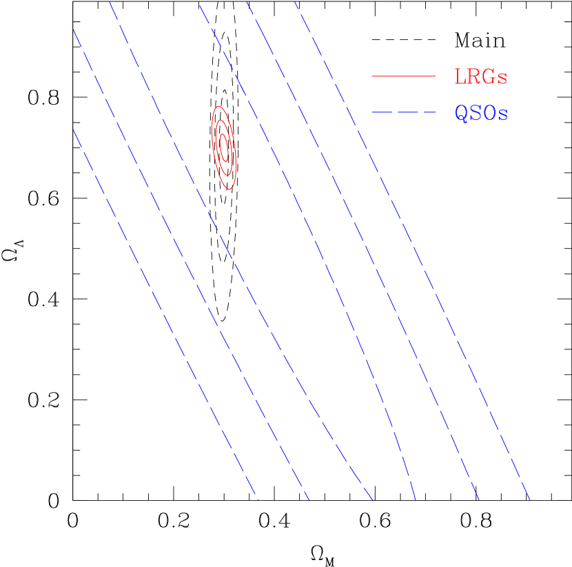
Figure 1: The concentration ellipses for the cosmological parameters $\Omega_{\rm M}$ and $\Omega_{\rm\Lambda}$. Expected 68%, 95%, 99.7% confidence levels are shown. Dashed lines are for main galaxies, solid lines for luminous red galaxies (LRGs), and long-dashed lines for quasars (QSOs).

Three contours for each sample represent the concentration ellipses of $\nu=1,2,3$ which correspond to expected $1\sigma$, $2\sigma$, $3\sigma$ constraints in the parameter space, as described in the previous section. One can notice that the LRGs impose the best constraint on the $\Omega_{\rm M}$–$\Omega_{\Lambda}$ plane. The main galaxies can only probe a shallow redshift region, so that the cosmological constant does not strongly contribute to the redshift-space clustering, and therefore is less constrained. Although the QSOs can probe deep redshifts, they are too sparse to detect the redshift-space clustering itself. The LRGs nicely have intermediate properties and are balanced between the depth and the density of the survey objects.

In Figure 2 we plot the expected errors when three parameters, $\Omega_{\rm M}$, $\Omega_{\rm\Lambda}$, $\Omega_{\rm B}/\Omega_{\rm M}$ are simultaneously evaluated.

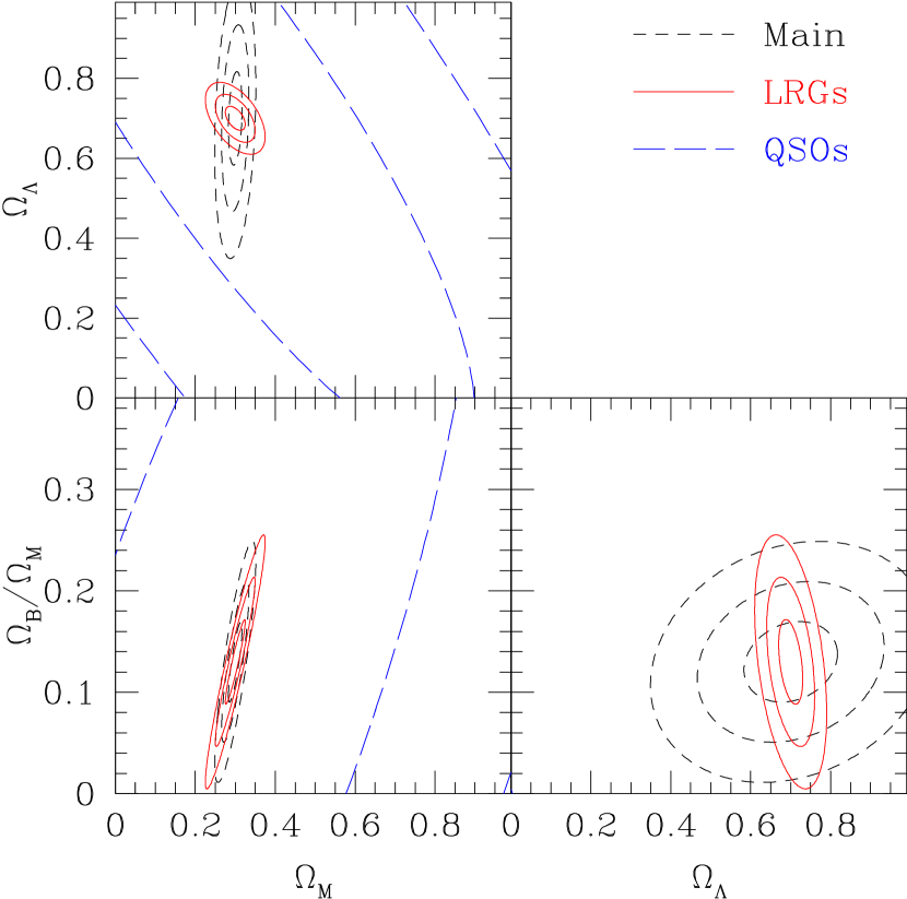
Figure 2: The marginalized 2D concentration ellipses when three cosmological parameters are simultaneously determined.

In each panel, marginalized errors are plot for each set of two parameters, as described in the previous section. In this case, the QSOs do not constrain each parameter well, because of their sparseness. Main galaxies and LRGs can impose similar constraints for the baryon fraction and the mass density parameter.

In Figure 3 we plot the expected errors when four parameters, $\Omega_{\rm M}$, $\Omega_{\rm\Lambda}$, $\Omega_{\rm B}/\Omega_{\rm M}$, $b$ are simultaneously evaluated.

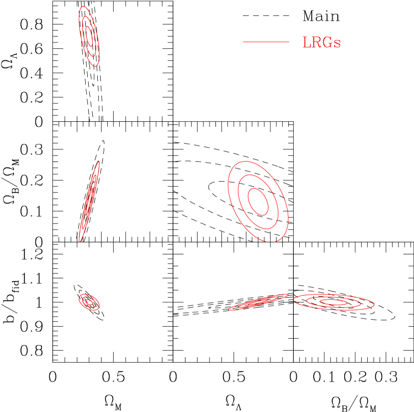
Figure 3: The marginalized 2D concentration ellipses when four cosmological parameters are simultaneously determined.

The results of the QSOs are not plotted just because the concentration ellipses are too large and comparable to the bounding boxes. In this Figure, the bias parameter $b$ is normalized by the fiducial values $b_{\rm fid}=1,2,2$ for each sample, just for convenience. The bias parameters in this Figure are assumed to be constants without redshift-evolution. If this is not the case, one can divide the sample into redshift bins, and the expected errors of bias parameter will be worse, according to the decrease of the sample volume. However, the error estimates of the other parameters in this Figure are approximately independent of the redshift evolution of the bias due to the marginalization over the bias parameter. This is because the information from cross terms in the redshift bins of $\sim 0.1$ are already ignored in our analysis, and the likelihood function with a fixed bias parameter is not too sensitive to the bias parameter Matsubara & Szalay (2001).

In Figure 4 we plot the expected errors, while simultaneously evaluating five parameters, $\Omega_{\rm M}$, $\Omega_{\rm\Lambda}$, $\Omega_{\rm B}/\Omega_{\rm M}$, $\sigma_{8}$, and $b$.

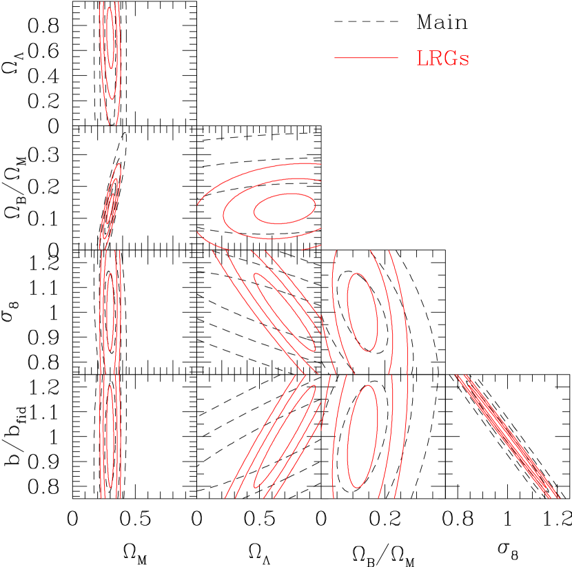
Figure 4: The marginalized 2D concentration ellipses when five cosmological parameters are simultaneously determined.

The bias parameter $b$ and the normalization $\sigma_{8}$ are strongly correlated because their main contribution to the correlation matrix is through the amplitude of the correlations which is proportional to $b^{2}{\sigma_{8}}^{2}$. In Figure 5 we plot the expected errors, while simultaneously evaluating another set of five parameters, $\Omega_{\rm M}$, $\Omega_{\rm\Lambda}$, $\Omega_{\rm B}/\Omega_{\rm M}$, $n$, and $b$.

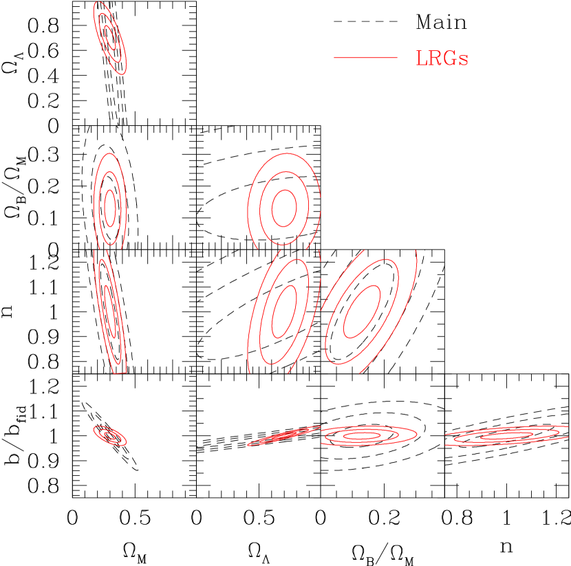
Figure 5: The marginalized 2D concentration ellipses when three cosmological parameters are simultaneously determined.

Any similar plot can be generated for an arbitrary set of simultaneously determined parameters. There are ${7\choose 1}+{7\choose 2}+\cdots+{7\choose 7}=127$ ways to choose which parameters are fixed, so that we need 122 figures more to be complete. Instead we have shown only several representative cases above. In Table 1 are given all the elements of our estimated seven-dimensional Fisher matrices from which all the information can be extracted according to the way described in the previous section.

Table 1: Normalized seven-dimensional Fisher Information matrices $F_{\alpha\beta}/(\theta_{\alpha}\theta_{\beta})_{\rm fid}$ for the SDSS main galaxies, LRG’s, and QSO’s.

Main	$\Omega_{\rm M}$	$\Omega_{\rm\Lambda}$	$h$	$\Omega_{\rm B}/\Omega_{\rm M}$	$n$	$\sigma_{8}$	$b$
$\Omega_{\rm M}$	$1040.$	$-25.8$	$675.$	$-161.$	$1050.$	$4080.$	$3200.$
$\Omega_{\rm\Lambda}$	$-25.8$	$37.9$	$2.38$	$-0.0284$	$14.0$	$-1090.$	$-989.$
$h$	$675.$	$2.38$	$619.$	$-148.$	$995.$	$978.$	$818.$
$\Omega_{\rm B}/\Omega_{\rm M}$	$-161.$	$-0.0284$	$-148.$	$36.0$	$-235.$	$-262.$	$-219.$
$n$	$1050.$	$14.0$	$995.$	$-235.$	$1640.$	$938.$	$792.$
$\sigma_{8}$	$4080.$	$-1090.$	$978.$	$-262.$	$938.$	$51600.$	$43200.$
$b$	$3200.$	$-989.$	$818.$	$-219.$	$792.$	$43200.$	$36600.$
LRG’s	$\Omega_{\rm M}$	$\Omega_{\rm\Lambda}$	$h$	$\Omega_{\rm B}/\Omega_{\rm M}$	$n$	$\sigma_{8}$	$b$
$\Omega_{\rm M}$	$1740.$	$513.$	$1680.$	$-398.$	$2710.$	$-2400.$	$-2310.$
$\Omega_{\rm\Lambda}$	$513.$	$804.$	$360.$	$-81.8$	$653.$	$-7420.$	$-6850.$
$h$	$1680.$	$360.$	$1730.$	$-418.$	$2760.$	$-1510.$	$-1370.$
$\Omega_{\rm B}/\Omega_{\rm M}$	$-398.$	$-81.8$	$-418.$	$103.$	$-661.$	$308.$	$280.$
$n$	$2710.$	$653.$	$2760.$	$-661.$	$4490.$	$-3390.$	$-3060.$
$\sigma_{8}$	$-2400.$	$-7420.$	$-1510.$	$308.$	$-3390.$	$88400.$	$78700.$
$b$	$-2310.$	$-6850.$	$-1370.$	$280.$	$-3060.$	$78700.$	$70500.$
QSO’s	$\Omega_{\rm M}$	$\Omega_{\rm\Lambda}$	$h$	$\Omega_{\rm B}/\Omega_{\rm M}$	$n$	$\sigma_{8}$	$b$
$\Omega_{\rm M}$	$10.2$	$11.5$	$9.28$	$-2.38$	$14.5$	$-27.5$	$-23.5$
$\Omega_{\rm\Lambda}$	$11.5$	$13.7$	$10.4$	$-2.60$	$16.3$	$-31.5$	$-27.5$
$h$	$9.28$	$10.4$	$8.72$	$-2.28$	$13.5$	$-24.2$	$-20.8$
$\Omega_{\rm B}/\Omega_{\rm M}$	$-2.38$	$-2.60$	$-2.28$	$0.614$	$-3.50$	$6.00$	$5.16$
$n$	$14.5$	$16.3$	$13.5$	$-3.50$	$21.0$	$-38.3$	$-32.9$
$\sigma_{8}$	$-27.5$	$-31.5$	$-24.2$	$6.00$	$-38.3$	$78.1$	$66.7$
$b$	$-23.5$	$-27.5$	$-20.8$	$5.16$	$-32.9$	$66.7$	$57.4$

The listed matrix elements are normalized by fiducial values as $F_{\alpha\beta}/(\theta_{\alpha}\theta_{\beta})_{\rm fid}$. Thus, the inverse of square-root of each diagonal element gives the fractional error relative to the fiducial value of each parameter when a single parameter is determined knowing the other parameters. The square-root of the diagonal elements of the inverse of any sub-matrix gives the fractional error of the parameters when corresponding parameters are simultaneously determined.

Basically, the LRG’s can impose constraints on each parameter comparable to, or even better than main galaxies. The reason that the main galaxies do not work so well (even though their number is 10 times larger than that of LRG’s) is that we only use the linear regime of the clustering. Therefore, the depth of the LRG sample is more critical for the parameter estimation than the higher density of the main galaxies. The quasars are hopeless when many parameters are simultaneously determined, because of their extreme sparseness. In this way, our analysis gives the idea how the dense sampling affects cosmological parameter estimations.

5 Conclusions

In this paper, we described a maximum-likelihood method to determine the cosmological parameters from apparent redshift-space clustering. We took advantage of the analytical formula for linear two-point correlations in redshift space with cosmological distortions. We introduced an accurate approximation in calculating the elements of the correlation matrix among cells in redshift-space. This step makes the method practically feasible in spite of the large dimensionality of the correlation matrices.

In the maximum-likelihood method, one can easily evaluate the expected parameter estimation errors in any sample from the Fisher information matrix. We have calculated the seven-dimensional Fisher matrix for three types of objects in the SDSS survey: main galaxies, LRGs and quasars. To illustrate the behavior of the multi-dimensional Fisher matrix we have used concentration ellipses in marginalized two-dimensional parameter space.

In this paper, we divided the survey volume into generic boxes in order to simplify the Fisher matrix estimation. We ignored the correlations between these sub-regions, so the constraints will improve somewhat if those correlations are properly included. However, the inversion of the resulting huge matrices can become extremely time-consuming. The use of the Karhunen-Loève (KL) transform is a practical strategy in this case. Such methods can also be used in a targeted data-compression role to find linear combinations of counts which retain as much information about the parameters as possible (Vogeley & Szalay, 1996; Tegmark, Taylor & Heavens, 1997; Matsubara, Szalay & Landy, 2000; Taylor et al., 2001).

The choice of the cell radius is somewhat arbitrary in this work. We choose the spherical cell with radius of $10{\hbox{$\,h^{-1}$}{\rm Mpc}}$ for galaxies and LRGs, which is the border of the linear regime. With larger cell radius, the validity of the linear theory increases and the shot noise is reduced. The cosmic variance, however, increases with cell radius. The parameter estimation is dominated by the highest signal-to-noise modes, which are at large wavelength, in particular for the case of the LRG sample. The high frequency modes close to pixel scales mostly contain shot noise after the KL transformation. As a result, we believe our conclusions are not sensitive to the choice of the cell radius. A fully accurate determination of the optimal choice of the cell radius depends on the behavior of the nonlinear effects, so that a comparison with numerical simulation is needed, beyond the scope of the current work.

We have considered three subsets of the SDSS redshift data, spanning a wide range of depth, sampling density and intrinsic clustering strength. We found, that for measuring cosmological parameters in the linear regime there is a clear optimum, represented by the intermediate-redshift LRG’s. The low spatial density of quasars is not overcome by their much larger depth, and the relatively small depth of the main SDSS galaxies is not compensated by their high sampling density – the redshift is not high enough to test curvature, and their cosmic variance is too large. The LRG sample, much smaller in numbers than the main sample, and much shallower than the quasars is an excellent compromise between sampling density and cosmological depth. The constraints derived from the LRGs are much tighter than for the other two samples.

The advantage of these intermediate-redshift objects, and the logic behind this optimum goes beyond the SDSS. In designing future redshift surveys, it is important to find the right balance between the density of objects and the survey depth. Their interplay can be quite complex, as we have shown here. The relation between accuracy and sky coverage is simple and can be estimated analytically.

References

- Alcock & Paczyński (1979) Alcock, C. & Paczyński, B. 1979, Nature, 281, 358
- Ballinger, Peacock & Heavens (1996) Ballinger, W. E. & Peacock, J. A. & Heavens, A. F. 1996, MNRAS, 282, 877
- Davis & Peebles (1983) Davis, M. & Peebles, P. J. E. 1983, ApJ, 267, 465
- de Bernardis et al. (2000) de Bernardis, P. et al. 2000, Nature, 404, 955
- Eisenstein & Hu (1998) Eisenstein, D. J. & Hu, W. 1998, ApJ, 496, 605
- Eisenstein et al. (2001) Eisenstein, D. J. et al. 2001, AJ, 122, 2267
- Feldman, Kaiser & Peacock (1994) Feldman, H. A., Kaiser, N. & Peacock, J. A. 1994, ApJ, 426, 23
- Hamilton (1992) Hamilton, A. J. S. 1992, ApJ, 385, L5
- Kaiser (1987) Kaiser, N. 1987, MNRAS, 227, 1
- Kendall & Stuart (1969) Kendall, M. G. & Stuart, A. 1969, The Advanced Theory of Statistics, Vol. 2 (London: Griffin)
- Lahav et al. (1991) Lahav, O., Lilje, P. B., Primack, J. R. & Rees, M. J. 1991, MNRAS, 251, 128
- Lightman & Schechter (1990) Lightman, A. P. & Schechter, P. L. 1990, ApJS, 74, 831
- Matsubara & Suto (1996) Matsubara, T. & Suto, Y. 1996, ApJ, 470, L1
- Matsubara (2000) Matsubara, T. 2000, ApJ, 535, 1
- Matsubara, Szalay & Landy (2000) Matsubara, T., Szalay, A. S. & Landy, S. D. 2000, ApJ, 535, L1
- Matsubara & Szalay (2001) Matsubara, T. & Szalay, A. S. 2001, ApJ, 556, L67
- Perlmutter et al. (1999) Perlmutter, S. et al. 1999, ApJ, 517, 565
- Riess et al. (1998) Riess, A. G. et al. 1998, AJ, 116, 1009
- Seljak & Zaldarriaga (1996) Seljak, U. & Zaldarriaga, M. 1996, ApJ, 469, 437
- Taylor et al. (2001) Taylor, A. N., Ballinger, W. E., Heavens, A. F. & Tadros, H. 2001, MNRAS, 327, 689.
- Tegmark, Taylor & Heavens (1997) Tegmark, M., Taylor, A. N., & Heavens, A. F. 1997, ApJ, 480, 22
- Therrien (1992) Therrien, C. W. 1992, Discrete Random Signals and Statistical Signal Processing, (New Jersey: Prentice-Hall).
- Vogeley & Szalay (1996) Vogeley, M. S. & Szalay, A. S. 1996, ApJ, 465, 34
- York et al. (2000) York, D. G. et al. 2000, AJ, 120, 1579