Numerical Simulations of MHD Turbulence
in Accretion Disks

Abstract

We review numerical simulations of MHD turbulence. The last decade has witnessed fundamental advances both in the technical capabilities of direct numerical simulation, and in our understanding of key physical processes. Magnetic fields tap directly into the free energy sources in a sufficiently ionized gas. The result is that adverse angular velocity and adverse temperature gradients, not the classical angular momentum and entropy gradients, destabilize laminar and stratified flow. This has profound consequences for astrophysical accretion flows, and has opened the door to a new era of numerical simulation experiments.

1 Introduction

Magnetized, differentially rotating plasmas are subject to a powerful linear instability, whose maximum growth rate is a factor of $\sim 10^{2}$ per orbit (Balbus & Hawley 1991). This is the magnetorotational instability, or MRI. Despite the fact that planar Couette flow is exquisitely sensitive to nonlinear disturbances and flow lamina quickly breakdown into turbulence, decades of investigation have failed to find any comparable mechanism in a nonmagnetized Keplerian disk. The problems is that local Coriolis forces are larger than the effective disruptive inertial force caused by the presence of shear. The result is that nonacoustic disturbances respond in a wavelike manner in a disk, whereas no such response is possible in nonrotating shear flow. Instead, the displacements of perturbed fluid elements are (linearly) unbounded, eventually becoming ensnared in the shear flow, feeding a breakdown to turbulence.

The astrophysical significance of this is associated with accretion sources. By dint of angular momentum conservation, accretion onto compact objects invariably involves differentially rotating flow with a centrifugal barrier enshrouding the central mass. The presence of a magnetic field leads to the development of the MRI, which causes fluid elements to lose their specific angular momentum, and leads to the accretion process itself. Happily, for the purposes of this conference, many of the details of this process may studied via large scale numerical simulations.

In this paper we will briefly review the history and contributions of numerical MHD simulations of accretion disks. Numerical investigations of this problem began in earnest only a decade ago, and their impact has been profound. They have taught us not only what happens in a highly complex accretion flow, by varying flow parameters we have often learned why it happens as well. As a recent example of this, we shall discuss in some detail the structure of nonradiating flows (associated with black hole accretion) that numerical simulations have revealed in the last year or so. The topic is important, fascinating, and not entirely free of controversy.

The review proceeds along the following outline. In §2, we review the physics of the magnetorotational instability in its most general form. §3 discusses simulations that focus on a local patch of an unstable Keplerian disk. By limiting dynamical range, these calculations may include more sophisticated physics. In §4, global MHD simulations are summarized. Given their much larger dynamical range requirements, it is not yet possible to treat the more complex fluids amenable to a local analysis, but even these simple fluids may be of astrophysical relevance. There is ample evidence now for a non-radiative flows at the Galactic Center, and there is reason to believe this is not a special case. We conclude with a summary in §5.

2 The Magnetorotational Instability

We begin with a review of the MRI (Balbus & Hawley 1998). The dynamics of this instability are very simple, involving only the notion of magnetic tension in the presence of rotational forces.

2.1 Formal Calculation

The simplest case involves an axisymmetric disk threaded by a weak, vertical magnetic field, $\vec{B}=B\vec{e_{Z}}$, where $\vec{e_{Z}}$ is a vector in the $Z$ direction. (We are using a standard $(R,\phi,Z)$ cylindrical coordinate system.) The undisturbed flow consists of fluid elements on circular orbits. We make a displacement $\vec{\xi}=(\xi_{R},\xi_{\phi},0)$ in the disk plane. The time and space dependence of the displacement is a simple plane wave,

$$\vec{\xi}=\vec{\xi^{\prime}}\exp(ikZ-i\omega t),$$ (1)

which defines the wavenumber $k$ and angular frequency $\omega$. The wave propagates along the magnetic field line at the Alfvén speed

$$v_{A}^{2}={B^{2}\over 4\pi\rho},$$

and is a consequence of the restoring field line tension $-(kv_{A})^{2}\vec{\xi}$.

We go into a frame rotating at the angular velocity $\Omega$ of a fiducial orbit. In this frame, in addition to the magnetic tension force, we must add a Coriolis force $-2\vec{\Omega}\vec{\times}d\vec{\xi}/dt$, and a centrifugal force $R\Omega^{2}\vec{e_{R}}$. The latter is exactly balanced by the inward gravitational force just at the location of the fiducial orbit, and the residual tidal force amounts to $-\vec{\xi}d\Omega^{2}/d\ln R$. The equations of motion for a fluid displacement are thus

$${d^{2}\xi_{R}\over dt}-2\Omega{d\xi_{\phi}\over dt}=-\left[(kv_{A})^{2}+{d\Omega^{2}\over d\ln R}\right]\xi_{R},$$ (2)

$${d^{2}\xi_{\phi}\over dt}+2\Omega{d\xi_{R}\over dt}=-(kv_{A})^{2}\xi_{R}.$$ (3)

The coefficients $\Omega$ and $d\Omega^{2}/d\ln R$ are now taken to be constant, since our calculation is local. Note as well that pressure forces are unimportant since $\vec{k}\vec{\cdot}\vec{\xi}=0$.

Plane wave solutions of these equations satisfy the dispersion relation

$$\omega^{4}-\omega^{2}[\kappa^{2}+2(kv_{A})^{2}]+(kv_{A})^{2}\left[(kv_{A})^{2}+{d\Omega^{2}\over d\ln R}\right]=0,$$ (4)

where $\kappa$ is known as the epicyclic frequency

$$\kappa^{2}=4\Omega^{2}+{d\Omega^{2}\over d\ln R}={1\over R^{3}}{d(R^{4}\Omega^{2})\over dR},$$ (5)

i.e., $\kappa^{2}$ is just proportional to the angular momentum gradient. In the absence of a magnetic field, fluid displacements would oscillate about their unperturbed circular orbit radius at a frequency $\kappa$. The displacements can easily be calculated, and they appear in the rotating frame as elliptical paths, with the elements moving in a retrograde sense relative to the unperturbed circular orbits. It is these “epicycles” that give $\kappa$ its name.

The relation (4) is a quadratic equation in $\omega^{2}$, and it is straightforward matter to show that if $d\Omega^{2}/dR<0$, there are $\omega^{2}<0$ unstable modes. By way of contrast, it is angular momentum, not the angular velocity, that must decrease outwards for instability in an unmagnetized disk. This has major astrophysical consequences, because disks in nature almost all have a specific angular momentum profile that rises with increasing radius, but an angular velocity profile that decreases in the same direction. Ignoring even a highly subthermal field in a stability analysis is a grave error, leading to qualitatively incorrect conclusions. Magnetized and unmagnetized fluids behave very, very differently.

The maximum growth rate of the instability is a quantity of interest,

$$|\omega_{max}|={1\over 2}\left|d\Omega^{2}\over d\ln R\right|,$$ (6)

which students of galactic structure will recognize as the Oort $A$ value. In a Keplerian disk it amounts to $0.75\Omega$, an enormous growth rate. It has been speculated that it is impossible for any instability feeding off differential rotation to grow more rapidly (Balbus & Hawley 1992).

2.2 Qualitative Description

The equations of motion have precisely the same form as those that emerge in a simple mechanical problem. Imagine two masses connected by a spring, in orbit about a central mass. If one replaces $(kv_{A})^{2}$ by a spring constant, say $K$, our systems are identical. This gives an easy way to envision the behavior of the instability, with magnetic tension acting like a spring obeying Hooke’s law.

Denote the first mass as $M_{1}$, and assume it is on an orbit slightly closer to the center than mass $M_{2}$, which orbits farther out. $M_{1}$ travels slightly faster than $M_{2}$ if the angular velocity increases inwards, and the spring tension pulls back on it. On the other hand, $M_{2}$ is is pulled forward in its orbital trek. This means that there is a positive torque pulling forward on $M_{2}$, and a retarding torque pulling back on $M_{1}$. Thus $M_{1}$ gains angular momentum, $M_{2}$ loses angular momentum. With additional angular momentum, $M_{2}$ (the outer mass) moves to a more distant orbit, while $M_{1}$ (the inner mass), moves to an orbit farther in. This stretches the spring yet further, the tension rises, and the process runs away. This is the underlying cause of the magnetorotational instability. Magnetized angular momentum transport is an intrinsically unstable process, because the more fluid elements separate, the greater the rate of angular momentum exchange that is driving the separation in the first place.

2.3 General Stability Criteria

It is possible to study the behavior of axisymmetric modes in great generality. By way of comparison, we first give the results for an unmagnetized gas. The local stability of adiabatic perturbations is then governed by the Høiland criteria (e.g. Tassoul 1978):

$$-{3\over 5\rho}(\vec{\nabla}P)\cdot\vec{\nabla}\ln P\rho^{-5/3}+{1\over R^{3}}{\partial R^{4}\Omega^{2}\over\partial R}\geq 0,$$ (7)

$$\left(-{\partial P\over\partial z}\right)\,\left({\partial R^{4}\Omega^{2}\over\partial R}{\partial\ln P\rho^{-5/3}\over\partial Z}-{\partial R^{4}\Omega^{2}\over\partial z}{\partial\ln P\rho^{-5/3}\over\partial R}\right)\geq 0,$$ (8)

which allow for the presence of both vertical and radial gradients in the host medium.

In the presence of a magnetic field, all angular momentum gradients are replaced by angular velocity gradients in the stability criteria (Balbus 1995):

$$-{3\over 5\rho}(\vec{\nabla}P)\cdot\vec{\nabla}\ln P\rho^{-5/3}+{\partial\Omega^{2}\over\partial\ln R}\geq 0,$$ (9)

$$\left(-{\partial P\over\partial z}\right)\,\left({\partial\Omega^{2}\over\partial R}{\partial\ln P\rho^{-5/3}\over\partial Z}-{\partial\Omega^{2}\over\partial z}{\partial\ln P\rho^{-5/3}\over\partial R}\right)\geq 0.$$ (10)

This generalizes the result found in our simple example from the previous section, that the angular velocity, not the angular momentum, must increase outward when $\Omega=\Omega(R)$. We find here that angular velocity gradients are quite generally the proper stability discriminants in a magnetized gas.

Finally we include the effect of a Coulomb conductivity. In the presence of a magnetic field, dilute astrophysical plasmas conduct heat only along magnetic field lines, and then of course only if there is a gradient along the field line. This is a regime of some relevance to black hole accretion sources, in which the flow is characterized by very high temperatures and low densities. In this case, we find that the stability criteria may be obtained from the previous simply by changing the entropy gradients to temperature gradients (Balbus 2001):

$$-{1\over\rho}(\vec{\nabla}P)\cdot\vec{\nabla}\ln T+{\partial\Omega^{2}\over\partial\ln R}\geq 0,$$ (11)

$$\left(-{\partial P\over\partial z}\right)\,\left({\partial\Omega^{2}\over\partial R}{\partial\ln T\over\partial Z}-{\partial\Omega^{2}\over\partial z}{\partial\ln T\over\partial R}\right)\geq 0.$$ (12)

Note that these requirements are independent of the thermal conductivity coefficient. This is a most surprising result: a nonrotating, adiabatic stratification of a temperature plus a small sprinkling of magnetic field is highly unstable! Figure (1) shows the results of a full nonlinear simulation of this instability, as far as it could be followed. The restriction that the heat flow only along field lines is critical here, as a scalar thermal conductivity (e.g. radiation) would serve only to stabilize perturbations by dissipation. Further discussion of this delicate point may be found in Balbus (2001).

Figure 1: Development of thermoclinic instability in a Schwarzschild-stable layer. Magnetic lines of force are shown after one Alfvén crossing time, initial seeding with rms 1% random initial vertical velocity perturbations. Initial thermal energy density is 1600 times magnetic; initial field lines are isothermal and horizontal; vertical grid runs from $z=1$ to $2$, initial temperature profile is $1/z$, gravitational field is $1/z^{2}$; $\chi$ is 0.05; grid is $128\times 64$. (From Balbus [2001], simulation performed by J. M. Stone.)

The three forms of the stability criteria show an “evolution” of replacing gradients of the extensive variables $S$ and $L$ with gradients the intensive quantities $T$ and $\Omega$. Changes in the former are energy sources,

$$dE=T\,dS+\Omega\,dL+...,$$ (13)

while changes in the latter are free energy sources,

$$d(E-TS-\Omega L)=-S\,dT-L\,d\Omega+...,$$ (14)

Gradients in the free energy generally mean that lower energy or higher entropy equilibrium states are nearby. When a dynamical path becomes available to these states, instabilities are triggered. Transitions are swift: in all cases, the characteristic growth times are dynamical, either a sound crossing or a shearing time.

3 Local Nonlinear Simulations

With the general stability conditions in hand, it is natural to ask what are the nonlinear consequences of their violation? In general the answer is turbulent flow, and further progress depends upon numerical simulation.

3.1 Governing Equations

Start with the fundamental $R$ and $\phi$ equations of motion:

$$\rho{\partial v_{R}\over\partial t}+\rho\vec{(v\cdot\nabla)}v_{R}-\rho{v_{\phi}^{2}\over R}=-\rho{\partial\Phi\over\partial R}-{\partial P_{tot}\over\partial R}+\vec{(B\cdot\nabla)}{B_{R}\over 4\pi}-{B_{\phi}^{2}\over 4\pi R},$$ (15)

$$\rho{\partial v_{\phi}\over\partial t}+\rho\vec{(v\cdot\nabla)}v_{\phi}+\rho{v_{\phi}v_{R}\over R}=-{1\over R}{\partial P_{tot}\over\partial\phi}+\vec{(B\cdot\nabla)}{B_{\phi}\over 4\pi}+{B_{\phi}B_{R}\over 4\pi R},$$ (16)

where

$$P_{tot}\equiv P+{B^{2}\over 8\pi}$$

is the total gas plus magnetic pressure. To leading order, the disk is a simple Keplerian system, with angular velocity

$$R\Omega^{2}(R)={GM\over R^{2}}\equiv{\partial\Phi\over\partial R}$$ (17)

where $M$ is the central mass. Thermal and magnetic forces are small compared with the central gravitational force, though of course this “smallness scale” is precisely the one we are concerned with! We may express this quantitatively as

$$|(v_{\phi}-R\Omega)|\sim c_{S}\ {\rm(sound\ speed)}\sim v_{A}\ll R\Omega.$$ (18)

Note that the azimuthally-averaged $\phi$ equation may be written

$$\rho{\partial(R\rho v_{\phi})\over\partial t}+\vec{\nabla}\cdot\left[\rho R\left(v_{\phi}\vec{v}-v_{A\phi}\vec{v_{Ap}}\right)\right]=0$$ (19)

where $\vec{v_{Ap}}$ is the poloidal Alfvén velocity, and the all the angular momentum density and flux are understood to be averaged quantities. The $\phi$-averaged radial angular momentum flux may be read off directly from equation (19):

$${\cal F_{J}}_{R}=R\langle\rho(v_{\phi}v_{R}-v_{A\phi}v_{AR})\rangle_{\phi},$$ (20)

which is an important quantity.

In the local approximation, the idea is to focus on a small patch of the disk, fixing the new origin to corotate with disk fluid orbiting at a particular angular velocity, $\Omega_{0}$. We measure all velocities relative to $R\Omega_{0}$. We ignore curvature effects in the local computational patch of interest. Formally, we work in the limit,

$$R\rightarrow\infty,\quad v_{\phi}\rightarrow\infty,\quad\omega\rightarrow{\rm finite.}$$ (21)

We define the velocity $\vec{w}$:

$$\vec{w}=\vec{v}-R\Omega_{0}\,\vec{e_{\phi}}.$$ (22)

The value of $R$ at which $\Omega=\Omega_{0}$ will be denoted $R_{0}$. In general we shall consider only small radial excursions from $R_{0}$,

$$R=R_{0}+x,\quad x\ll R_{0}.$$ (23)

Thus,

$${R}\Omega_{0}^{2}-{\partial\Phi\over\partial R}=R(\Omega_{0}^{2}-\Omega^{2}(R))\simeq-x{d\Omega^{2}\over d\ln R}_{0}$$ (24)

to leading order. Local Cartesian coordinates can be defined by lining the $x$ and $y$ axes along $R$ and $\phi$. In a frame rotating at $\Omega_{0}$, the local equations of motion for $w_{X}$ and $w_{Y}$ are

$${\partial w_{X}\over\partial t}+\vec{w}\cdot\vec{\nabla}{w_{X}}-2\Omega w_{Y}+x{d\Omega^{2}\over d\ln R}=-{1\over\rho}{\partial P_{tot}\over\partial x}+\vec{B}\cdot\vec{\nabla}B_{X}$$ (25)

$${\partial w_{Y}\over\partial t}+\vec{w}\cdot\vec{\nabla}{w_{Y}}+2\Omega w_{X}=-{1\over\rho}{\partial P_{tot}\over\partial y}+\vec{B}\cdot\vec{\nabla}B_{Y}$$ (26)

The forms of the remaining dynamical equations remain unaffected by the change to rotating coordinates. They are the $Z$ equation of motion

$${\partial w_{Z}\over\partial t}+\vec{w}\cdot\vec{\nabla}{w_{Z}}=-{1\over\rho}{\partial P_{tot}\over\partial Z}+\vec{B}\cdot\vec{\nabla}B_{Z},$$ (27)

the equation of mass conservation

$${\partial\rho\over\partial t}+\vec{\nabla}\cdot(\rho\vec{w})=0,$$ (28)

the internal energy equation,

$$(\gamma-1)\rho\left({\partial\ \over\partial t}+\vec{w}\cdot\vec{\nabla}\right){P\over\rho}=-P\vec{\nabla}\cdot\vec{w}$$ (29)

The induction equations for the magnetic field lose terms of relative order $w/R\Omega$:

$${\partial B_{i}\over\partial t}+\vec{w}\cdot\vec{\nabla}B_{i}=\vec{B}\cdot\vec{\nabla}w_{i}$$ (30)

where $i=X,Y,Z$.

The set of equations (25)–(30) completely describes the local behavior of a magnetized accretion disk. We must first, however, specify the boundary conditions (BC) at the edges of the computational domain. The simplest approach is to use hard walls at each of the radial, azimuthal, and vertical boundaries. The first nonlinear numerical investigations of local accretion disk behavior were those of Hawley & Balbus (1991), who used hard wall BC. These first simulations were highly restrictive, but sufficed to demonstrate the existence of the weak field MRI, and confirm its analytic growth rates and its independence of an azimuthal field. These simulations used a vertical field and more complex loop geometries as starting configurations. Because no periodic BC were needed, these early simulations actually retained the curvature terms in the equations, so that non WKB terms were present. The detailed agreement between analytic calculation and numerical results left no doubt whatsoever of what was then a completely unexpected result: the combination of Keplerian rotation and a weak magnetic field is extremely unstable.

Extended simulations require what are known as shearing-box BC. In this approach, the azimuthal boundary conditions are always periodic. Vertical BC may be taken either as periodic or pure outflowing, depending upon the problem on interest. Because of the presence of large scale shear, the radial BC are more complex (Hawley, Gammie, & Balbus 1995). They may be described as “quasi-periodic:” the computational domain is thought of as one brick in a wall extending to infinity, each brick with the same fluid configuration as the next. The velocity shear is continuous across the entire brick wall, so a layer of bricks must slide with respect to the layer above and below! As one layer slides over another, a fluid element leaving the computational domain is replaced by its image on the opposite wall, but not at the azimuth it has just vacated. Instead it reappears at the azimuth from the sliding brick in contact with the computational domain. The mathematical formulation of these BC may be found in Balbus & Hawley (1998).

3.2 Local Axisymmetric Flow

To run simulations over many local shear times, the shearing box formalism must be implemented. This was first done by Hawley & Balbus (1992) for two-dimensional axisymmetric flow. A surprise emerged. Though the evolution of an initial uniform vertical magnetic field was in complete accord with analytic theory in the linear stages of its development, the nonlinear stages hardly appeared turbulent at all. In fact, the linear stage seemed to continue indefinitely, with exponentially growing streaming motions persisting. This contrasted sharply with the nonlinear behavior of a shearing box starting with a vertical field whose mean value was zero—half upwards and half downwards say, or sinusoidally varying. In that case, turbulence quickly developed after a few linear growth times, and then gradually decayed, leaving no field at all at the end of the simulation!

This behavior can be understood with the help of Cowling’s anti-dynamo theorem (Moffatt 1978). The theorem states that dynamo amplification is impossible in an isolated, dissipative axisymmetric system. To understand what is meant by “isolated,” we work with the azimuthal component of the vector potential, denoted $A$. In axisymmetry, this component alone suffices to determine the poloidal magnetic field. The mathematical heart of the theorem is that in the absence of resistance, the integrated form of Faraday’s induction equation may be manipulated into the form

$${\partial\ \over\partial t}\int A^{2}\,dV=-\int A^{2}\,\vec{v}\cdot\vec{dS}$$ (31)

where the left integral is over a volume containing the fluid (perhaps infinite), and the right integral is over a bounding surface (perhaps at infinity). If periodic boundary conditions are used, or if $A^{2}$ falls off sufficiently rapidly, then the surface integral vanishes. Hence, the average of $A^{2}$ remains constant for the fluid. The presence of any dissipation then causes an inevitable decline; there is nothing to offset it.

When the mean vertical field vanishes, the vector potential satisfies smooth periodic boundary conditions, and the anti-dynamo theorem applies directly. The magnetic field depends upon derivatives of $A$, and its growth therefore requires a sort of continuous kneading of the fluid, bringing different values of $A$ (which absent dissipation is a fluid element label) ever closer together. This continues on smaller and smaller scales, but eventually the grid scale is hit, and growth ceases at that point, with reconnection ensuing.

The presence of a nonvanishing mean magnetic field implies that $A$ is nonperiodic: it must have a component proportional to $x$. Since periodic boundary conditions no longer hold, the surface integral in equation (31) no longer vanishes, and poloidal field components may grow at the expense of the free energy of differential rotation. There is nothing unphysical about this set-up; real disks certainly can be threaded by a magnetic field. The question is do such disks really exhibit the streaming behavior discussed above?

This was examined authoritatively by Goodman & Xu (1994). These authors pointed out a remarkable fact: starting with a vertical field, linear plane wave eigensolutions are in fact exact nonlinear solutions to the equations of motion. In the local approximation, the gas really does appear to act like two orbiting masses connected by a spring. The existence and persistence in two dimensions of coherent disk streams provided an explanation for a recurring puzzling behavior seen in a number of earlier axisymmetric global MHD disk simulations. Uchida & Shibata (1985) and Shibata & Uchida (1986) were interested in the creation of MHD jets and investigated this problem by threading a disk of gas with a vertical magnetic field. By imparting less than the Keplerian value of the angular momentum to the orbiting fluid elements, they hoped to duplicate the effects of slow radial accretion—but without turbulence. The infall produced radial fields that became wrapped up by differential rotation into strong toroidal fields, whose gradients in turn drove dynamical outflows along the vertical field lines. Some of these simulations, however, began with a Keplerian disk embedded in a vertical magnetic field. Such disks also collapsed on a dynamic time scale. At the time, the reason for this was not at all clear. This may now be understood as a global manifestation of the streaming solutions studied by Goodman and Xu (1994).

The question was whether in three dimensions the fluid behavior will prove to be qualitatively different from the two dimensional case. Will the streams remain stable in three dimensions? Goodman & Xu noted that this ostensibly nonlinear question reduces to a linear stability problem, but a linear stability problem perturbed about a most unusual equilibrium solution. The presence of vertically periodic velocity streams renders the problem amenable to Floquet analysis (Bender & Orszag 1978), for which powerful mathematical techniques are available. The conclusion was that the new equilibrium of streaming motions should be unstable. The most important instability is a magnetized Kelvin-Helmholtz mode, which appears for radial wavelengths in excess of the streaming equilibrium flow’s vertical wavelength.

3.3 Local Three-Dimensional Simulations

To determine the ultimate fate of the streams of the Goodman-Xu solution or to study dynamo amplification requires implementation of three-dimensional MHD codes. By now, many shearing box studies have been carried out, and a wide variety of models explored. The simplest consists of a homogeneous box, in which only the radial component of the large scale gravitational field is retained, and the magnetic field is initially uniform (Hawley et al. 1995; Matsumoto & Tajima 1995). The initial field geometry in these studies had some combination of vertical and toroidal components. A more complicated initial field configuration, important for understanding dynamo activity, is to let the initial field have a random character with vanishing mean (Hawley, Gammie, & Balbus 1996). The presence of the vertical component of the gravitational field produces a density stratification (Brandenburg et al. 1995; Stone et al. 1996; Matsuzaki et al. 1997), which introduces the possibility of magnetic buoyancy, a new effect. Furthermore, by bringing the pseudoscalar quantity $\Omega\cdot\vec{\nabla}\rho$ into the problem, stratification breaks chiral symmetry, i.e., the flow acquires a “handedness.” This result is potentially important for the development of local mean helicity in the turbulence, a feature upon which much of classical kinematic dynamo theory is based (Moffatt 1978).

Stone et al. (1996) carried out a series of such simulations spanning two vertical scale heights in an initially isothermal disk. With the onset of the MRI, magnetic field rises out of the disc to establish a highly magnetized corona. The amplitude of the turbulence near the midplane is determined more by local dissipation than by buoyant losses, and the resulting stress levels are not greatly modified from the nonstratified simulations. The presence of a corona, however, could have important observational consequences if a significant amount of dissipational heating occurs there. Concerns about the effects of the close-in vertical boundary conditions led Miller & Stone (2000) to carry out simulations with a larger computational domain covering 5 scale heights above and below the equator. They demonstrated that indeed a strongly magnetized corona ($P_{\rm gas}\ll P_{\rm mag}$) forms naturally from little more than a disk and a weak seed field.

Three-dimensional studies also show the breakdown of the two-dimensional streaming solutions (Hawley et al. 1995). If the computational box is large enough to allow an unstable radial wavelength, streaming is disrupted within a few orbits, as the Kelvin-Helmholtz instability noted by Goodman & Xu (1994) leads to fluid turbulence, which is the basis of significant outward angular momentum transport. This is because the turbulence is inherently anisotropic; perturbations in the $x$ and $y$ components of the magnetic field and the velocity are highly correlated. Velocity power spectra of the simulations are weighted toward the lowest wavenumbers, i.e., there are significant fluctuations on scales comparable to the computational domain size. These large-scale fluctuations contain most of the magnetic energy and contribute the lion’s share of the stress.

Angular momentum is transported outward by the the MRI. To understand what is meant by that let

$$\vec{v}=R\Omega(R)\vec{e_{\phi}}+\vec{u}$$ (32)

i.e., $\vec{u}$ is the velocity in excess of the local Keplerian rotation. (Note that $\vec{w}$ is by contrast the velocity in excess of the local solid body rotation $R\Omega_{0}\vec{e_{\phi}}$.) Then the radial angular momentum flux from equation (20) is

$${\cal F_{J}}_{R}=R^{2}\Omega\langle\rho u_{R}\rangle_{\phi}+R\langle\rho(u_{R}u_{\phi}-v_{AR}v_{A\phi})\rangle_{\phi}.$$ (33)

The first term is simply the Keplerian angular momentum carried directly by the mass accretion. The second term is transport that is present whether or not there is any accretion present. This need not imply that an individual fluid element is losing angular momentum (though it generally is). In its linear stage, an axisymmetric unmagnetized convective instability transports angular momentum by having low and high angular momentum fluid elements interpenetrate, with no net mass flux. This means an inward angular momentum flux in a Keplerian disk, a result which is preserved in nonlinear three-dimensional simulations (Stone & Balbus 1996).

3.4 Radiative Effects

In general, thermal diffusion effects are not included in simulations. If the object of study is a classical optically thick Keplerian disk, this is a sensible approach to the dynamics. Radiative diffusion regulates the vertical temperature profile of the disk, but it does not greatly influence dynamical stability.

The linear stability of a magnetized, stratified, radiative gas was recently addressed by Blaes & Socrates (2001). Despite the complexity of the full problem, the MRI emerges at the end of the day unscathed, its classical stability criterion $d\Omega^{2}/dR>0$ remaining intact. The maximum growth rate can be lowered however, particularly when the azimuthal field approaches or exceed thermal strength. (The same is true for the ordinary MRI, as shown by Blaes & Balbus [1994]).

The nonlinear problem has been carried through by Turner, Stone, & Sano (2002), who set up a local, radiative, axisymmetric, shearing box flow. The linear calculations of Blaes & Socrates (2001) were confirmed in detail, and the nonlinear flow was analyzed. As in standard MRI simulations, the stress is dominated by the Maxwell component, which is a factor of a few larger than the Reynolds terms. Photon diffusion plays a dual role in keeping the matter nearly isothermal, and in creating over-dense clumps of gas of thermally dominated gas. The clumping occurs when radiation pressure support is lost via diffusion on a dynamical time scale at large wave numbers. In this regime, radiative disks may be highly inhomogeneous. At larger optical depths and longer diffusion times, the disks look similar to their nonradiative counterparts.

3.5 Low Ionization Disks

Protostellar disks, and possibly cataclysmic variable disks, contain regions of low ionization fraction—so low that the assumptions of ideal MHD break down. Ohmic dissipation becomes important, together with the Hall inductive terms. (The latter arises because the distinction between the mean electron and mean fluid velocities becomes important.) The effect of Hall electromotive forces on the MRI have been studied by Wardle (1999) and by Balbus & Terquem (2001). Nonlinear numerical simulations including ohmic resistivity have been done by Fleming, Stone , & Hawley (2000); Sano & Stone (2002) have done simulations including both the ohmic and Hall processes. It can be shown that under rather general conditions, if Ohmic dissipation is important, Hall electromotive forces are also important (Balbus & Terquem 2001; Sano & Stone 2002).

The most interesting feature introduced by Hall electromotive forces is helicity: the relative orientation of the angular velocity $\vec{\Omega}$ and magnetic field $\vec{B}$ vectors matters (Wardle 1999; Balbus & Terquem 2001). The key point is that $\vec{\Omega}\cdot\vec{B}>0$ configurations raise the maximum growth rate in the presence of ohmic losses, and this aligned configuration results in more vigorous transport in the local axisymmetric simulations of Sano & Stone (2002). In configurations where $\vec{\Omega}\cdot\vec{B}$ vanishes on average, the level of turbulence is much more sensitive to the size of the ohmic dissipation term.

In the simulations of Fleming et al. (2000) critical magnetic Reynolds number $Re_{M}$ emerged below which turbulence is suppressed. ($Re_{M}$ is defined here as the ratio of the product of the scale height and sound speed to the resistivity.) When the mean field vanishes, $Re_{M}$ was found to be surprisingly high, $\sim 10^{4}$. In the presence of a mean field, the critical $Re_{M}\sim 10^{2}$. The interesting and important question is whether the inclusion of Hall electromotive forces changes these numbers by lowering them, i.e., making it easier to support turbulence. The Sano & Stone (2002) axisymmetric simulations did not reveal a large change, but questions on the maintenance of turbulence more properly await a three-dimensional treatment.

4 Global Disk Simulations

Full global simulations are a demanding computational problem, requiring extended evolutions at high resolution. The fundamental difficulties with global simulations are worth reiterating. First one has a severe problem with length scales. The goal is to evolve accretion disks from first principles, which means computing the angular momentum transport self-consistently. Angular momentum transport is due to MHD turbulence, and the most-unstable MRI modes will typically be much smaller than the disk pressure scale height $H$. One would also like to resolve the turbulent cascade through its inertial range, if possible. The disk itself extends from the black hole horizon, $r_{S}$, out to thousands of horizon radii. Since all time scales are more or less $\propto\Omega$, Kepler’s law imposes a difficulty as well.

One must be practical and work within well-chosen limitations. It is often helpful to forgo density stratification, for example. One may also restrict the dimensionality of the problem, by adopting axisymmetry. Finally, and most critically, one must make a judicious choice of problem before embarking on a full global simulation.

4.1 Two-Dimensional Simulations

Axisymmetric MHD disk simulations have been used extensively in the past, particularly to study jet formation processes. Such simulations date back at least to Uchida & Shibata (1985). It is only more recently that two-dimensional simulations have directed primarily at the internal dynamics of the disk itself and the resulting accretion flow, rather than to the launching and collimation of jets.

From the astrophysical side, there has been considerable recent interest in under-luminous accreting compact objects, inspired in no small part by X-ray observations of the Galactic center (Melia & Falcke 2001). Despite the inferred presence of a $2\times 10^{6}\,M_{\odot}$ mass black hole, little of the expected radiation has been detected by Chandra. If the gas is able to radiate more rapidly than it accretes, there seems little doubt that it forms a thin Keplerian disk along the lines of Shakura & Sunyaev (1973). If the flow is either too optically thick for the radiation to diffuse outward over an accretion time, or too optically thin to radiate, then the fate of the gas is much less clear. Several ideas have circulated in the literature, dating from the earliest days of accretion theory. A small sample: Pringle & Rees (1972), Ichimaru (1977), Begelman & Meier (1982), Rees et al. (1982), Abramowicz et al. (1988), Narayan & Yi (1994, 1995), Narayan, Igumenschev, & Abramowicz (2000); Abramowicz et al. (2002).

From the numericist’s perspective, it is a most welcome development that there is evidence for, and intense interest in, nonradiating flows. For this is precisely the type of flow that is well-suited to numerical simulation. The first MHD simulations of nonradiating accretion flows were carried out by Stone & Pringle (2001). Here, accretion begins from an initial equilibrium torus, and is driven by MHD stresses arising from the onset of the MRI. The initial infall phase is relatively smooth and dominated by the vertical field “channel flow” of the MRI (cf. §3). Subsequent evolution is decidedly turbulent. The resulting flow consists of an approximately barotropic disk near the midplane, with constant $\Omega$ contours parallel to cylindrical radii. There was no strong correlation between the specific angular momentum and entropy, as was found in hydrodynamical simulations (Stone, Pringle, & Begelman 1999). A substantial magnetized coronal outflow enveloped the disk. Finally, there was very little difference in the character of the solution if dissipative losses were retained as heat or simply ignored.

While most of these features were destined to survive in three-dimensional runs, two dimensions is generally a significant limitation for the study of MHD turbulence Hawley (2000). Poloidal magnetic field cannot be indefinitely maintained in axisymmetry, by the anti-dynamo theorem (e.g., Moffat 1978). Indeed, toward the end of the Stone & Pringle (2001) simulations the turbulence clearly begins to die away. A more minor concern is that axisymmetric simulations tend to over-emphasize streaming modes, which produces coherent radial magnetized flows rather than the more generic MHD turbulence. Finally, toroidal field instabilities cannot be simulated in axisymmetry. Nothwithstanding these limitations, by allowing a rapid investigative turnover of plausible accretion scenarios, two-dimensional simulations have proven to be a valuable tool, and a remarkably reliable one as well.

4.2 “Cylindrical Disks”

The “cylindrical disk” is a global three-dimensional system allowing for full radial and azimuthal dynamics, but ignoring the vertical component of the central gravitational field. Hence, there is no vertical stratification. Turbulence and magnetic field can be easily sustained however, and far fewer vertical grid zones are required compared with true three-dimensional simulations.

Armitage (1998) carried out the first such a calculation using the standard ZEUS code and a grid covering the full $2\pi$ in azimuth, running from $R=1$ to 4 with a reflecting inner boundary and an outflow outer boundary, and covering a length of 0.8 in $z$. Vertical boundary conditions were periodic. The initial magnetic field was vertical and proportional to $\sin(kR)/R$, with the sine function argument linearly varying over $2\pi$ between $R=1.5$ and 3.5. From this initial state, turbulence rapidly developed along with significant angular momentum transport.

A more extensive set of cylindrical simulations (Hawley 2001) reaffirmed many of the conclusions of the local box models for accretion disk turbulence driven by the magnetorotational instability, as well as testing several technical aspects of global simulations. Because the driving instability is local, a reduction in the azimuthal computational domain to some fraction of $2\pi$ does not create large qualitative differences. Similarly, the choice of either an isothermal or adiabatic equation of state has little impact on the initial development of the turbulence. Simulations that begin with vertical fields have greater field amplification and higher ratios of stress to magnetic pressure compared with those beginning with toroidal fields.

Recently, cylindrical disk calculations have been to the problem of the star-disk boundary layer (Armitage 2002; Steinacker & Papaloizou 2002). Such simulations represent an important step forward, as previous studies of boundary layers were modeled by a hydrodynamic viscosity. Significant dynamo activity was reported by both sets of investigators. In particular, Armitage (2002) finds an order of magnitude larger field energy density in the boundary layer compared with the average disk field. Dissipative heating in the boundary layer has yet to be simulated.

4.3 Three-Dimensional Simulations

Global three-dimensional MHD disk simulations with full vertical structure were presented by Hawley (2000). These models started with equilibrium tori containing either a weak poloidal or a weak toroidal magnetic field. A torus is a useful initial condition for global simulations because it can be well-resolved and wholly contained within the grid. The thickness of the torus depends upon the angular momentum distribution, with constant specific angular momentum $l$ associated with the thickest tori. Such a structures may actually be generic in active galactic nuclei, where the feed an an inner disk (Krolik 1999). As the system evolution proceeds, the MRI develops rapidly. Stresses are dominated by the Maxwell component (a factor of several larger than the Reynolds stress), which immediately redistribute angular momentum from the initial non-Keplerian profile to nearly Keplerian state. At later times, the disks show rapid time variability, tightly wrapped, low-$m$ spiral structure, and significant internal stress.

Machida, Hayashi, & Matsumoto (2000) studied the evolution of a constant angular momentum torus containing toroidal magnetic field. Turbulence soon develops and magnetically dominated ($\beta<1$) filaments form. The buoyancy of such fields leads to the development of a strongly magnetized corona.

Steinacker & Henning (2001) have recently revisited the question of the influence of a large-scale vertical field on an accretion disk, previously studied in axisymmetry. They found strong accretion in the disk (the authors described it as a collapse) driven by the MRI. Coupling to a magnetized corona drives outflows, with the degree of collimation depending on the strength of the field.

The nature of the magnetic stress near the marginally stable orbit of black hole ($6GM/c^{2}$ for a Schwarzschild hole) has received renewed attention. This disk hydrodynamic treatments using a turbulent viscosity lead to a vanishing stress in this region (Abramowicz & Kato 1989), but matters can be more complicated when magnetic stresses are involved (e.g. Novikov & Thorne 1973; Gammie 1999; Algol & Krolik 2000). The question of what happens to the stress is of interest because of the possibility of extracting energy from the hole’s rotation and communicating it to the disk. It can be addressed via three-dimensional MHD simulations.

Hawley & Krolik (2001, 2002) investigated the evolution of a magnetized accretion torus lying near the marginally stable orbit in a pseudo-Newtonian model potential for the black hole (Paczyński & Wiita 1980). The work focused on the behavior of the stress as the gas flows through the “plunging region” inside of the marginally stable orbit. These simulations used the finest three-dimensional resolution to date, with up to $256\times 64\times 192$ zones in $(R,\phi,z)$, and as many as 70 radial grid zones lying between the marginally stable orbit and the horizon. They find that, in contrast to standard models, the disk does not sharply truncate at the marginally stable orbit, nor does the stress vanish. For both poloidal and toroidal fields the stress actually increases somewhat in the plunging region. The nature of the flow shifts from MHD turbulence to flux freezing, and in doing so drags out and shears the field lines, increasing the correlation between $B_{R}$ and $B_{\phi}$, and hence the Maxwell stress. Variability over large spatial scales is the rule here, over a broad range of time scales.

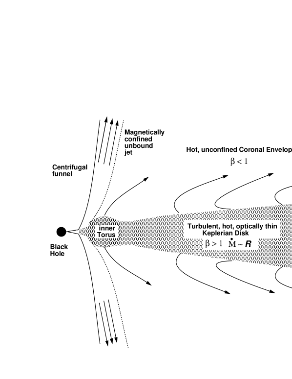
Figure 2: A schematic diagram of a nonradiative accretion flow, highlighting its principal features. A turbulent, nearly Keplerian gas-dominated hot disk is surrounded by an active, diffuse, magnetic-dominated coronal envelope. Near the marginally stable orbit, the flow thickens into a small inner torus. A centrifugally-evacuated funnel lies along the axis, surrounded by a jet confined by magnetic pressure in the corona. From Hawley & Balbus (2002).

The general accretion problem occurs over much larger scales, at least hundreds of gravitational radii. This global nonradiative MHD accretion flow, first considered in two dimensions by Stone & Pringle (2001), was extended to three dimensions in Hawley, Balbus & Stone (2001) and Hawley & Balbus (2002). The accretion flow originates with a constant specific angular momentum torus initially centered at 100 gravitational radii. MHD turbulence ensues and the resulting flow seems to settle into three well-defined dynamical structures. The main accretion is through a hot, thick, rotationally-dominated Keplerian disk. The MRI is so efficient at transporting angular momentum, the transformation from constant angular momentum to Keplerian profile occurs within a few orbital times at the pressure maximum. Evidently, Keplerian profiles are characteristic of warm and cool disks alike. The total pressure scale height in this disk is comparable to the vertical size of the initial torus. Surrounding this disk is a magnetized corona with vigorous circulation and possibly outflow. Gas pressure dominates only near the equator; magnetic pressure is more important in the surrounding corona. Finally, a magnetically-confined jet forms along the centrifugal funnel wall. Runs with and without Ohmic heating were performed; very few differences were found. The flow was somewhat hotter in the resistive runs, and the turbulence slightly subdued, but the dynamics remain dominated by MHD turbulence. There was no evidence of a convective envelope (Abramowicz et al. 2002).

Figure (2) shows schematically the appearance of the disk, corona, and jet as they appear in a typical run. The inner torus is pressure-thickened, but remains predominately supported by rotation. It is a highly transitory structure, forming and collapsing over the course of the simulation.

Contours of specific angular momentum are shown in figure (3). The disk emerges sharply in this diagram as the zone of cylindrical contours. This appears to be a consequence of the relatively small magnetic to thermal energy density ratio, and a barotropic equation of state.

Figure 3: Contours of azimuthally-averaged specific angular momentum. The disk is associated with the contours stratified nearly on cylinders. From Hawley & Balbus (2002).

Figure (4) is a momentum plot of the inner 20 gravitational radii of the disk, showing the internal dynamical structure of the inner torus. The distinct jet structure stands out particularly clearly.

Figure 4: Azimuthally-averaged momentum vectors in the within 20 gravitatinal radii of the black hole. The overlaid contour is density, showing the shape of the inner torus. The jet outflow along the centrifugal barrier is clearly evident. The magnetic pressure in the corona confines the jet externally. From Hawley & Balbus (2002).

5 Summary

Our understanding of accretion phenomena has grown enormously in the past decade, and the physical process underlying the anomalous viscosity of accretion disks have been elucidated. Indeed, “anomalous viscosity” is a misnomer, since magnetic fields do so much more than fill the role occupied by a hydrodynamical Navier-Stokes viscosity, and we should move away from this mode of thought. Magnetized fluids are far too subtle for this approach to be successful.

The combination of a magnetic field and outwardly decreasing differential rotation is highly unstable, as is the combination of a magnetic field and an upwardly decreasing temperature profile. Local simulations of Keplerian disks show that this magnetorotational instability leads to a turbulence-enhanced stress tensor that transports energy and angular momentum outwards, allowing accretion to proceed. The typical dimensionless value of the stress (normalized to a fiducial pressure) ranges from $5\times 10^{-3}$ to $0.6$ depending upon field geometry, and is highly variable in both space and time. Local simulations have become very sophisticated in the class of problems they are able to investigate. Work has begun on the local disk dynamics of radiation-dominated and non-ideal MHD systems.

Fully global three-dimensional MHD simulations are now a reality. These runs show that initially non-Keplerian angular momentum distributions rapidly evolve to Keplerian. Efficient angular momentum transport builds up rotation in the outer regions in the early stages, and the gas expands. Any initial radial pressure gradient is “inflated” to zero, and a Keplerian distribution emerges.

Chandra observations have provided compelling evidence that very low luminosity accretion flows are present in Nature, and such flows are amenable to numerical investigation. The most detailed studied to date (Hawley & Balbus 2002) reveals a three component structure: a warm Keplerian disk, a highly magnetized corona, and an axial jet. None of these structures were present in the initial condition, which is a simple constant angular momentum torus located 100 gravitational radii from the hole. Significant fluctuations in all flow quantities are present, both in time and in space. There was no indication that thermal convection was dominating the dynamical flow structure (Abramowicz, et al. 2002).

The results of global three-dimensional MHD numerical simulations comprise a vast and extremely useful data base, a true numerical laboratory. At the time of this writing, relatively little has been done to translate the formal numerical flows into photons impinging upon instruments. The exploitation of this largely untapped resource should provide advances as singular as those of the last extraordinary decade.

Acknowldgements

Our research is supported by NASA grants NAG-10655, NAG5-9266, and NSF grant AST-0070979. The authors are most grateful to the editors E. Falgarone and T. Passot for the their patience and forbearance.

References

- (1) Abramowicz, M. A., Czerny, B., Lasota, J.-P., & Szuszkiewicz, E. 1988, ApJ, 332, 646
- (2) Abramowicz, M. A., Igumenschev, I. V., Quataert, E., & Narayan, R. 2002, ApJ, 565, 1101
- (3) Algol, E., & Krolik, J. H. 2000, ApJ, 528, 161
- (4) Armitage, P. 1998, ApJ, 501, L189
- (5) Armitage, P. 2002, MNRAS, in press (astro-ph/0110670)
- (6) Balbus, S. A. 1995, ApJ, 453, 380
- (7) Balbus, S. A. 2001, ApJ, 562, 909
- (8) Balbus, S. A., & Hawley, J. F. 1991, ApJ, 376, 214
- (9) Balbus, S. A., & Hawley, J. F. 1992, ApJ, 392, 662
- (10) Balbus, S. A., & Hawley, J. F. 1998, RMP, 70, 1
- (11) Balbus, S. A., & Terquem, C. 2001, ApJ, 552, 235
- (12) Bender, C. M., & Orszag, S. A. 1978, Advanced Mathematical Methods for Scientists and Engineers (New York: McGraw–Hill), p. 560
- (13) Begelman, M. C., & Meier, D. L. 1982, ApJ, 253, 873
- (14) Blaes, O. M., & Balbus, S. A. 1994, ApJ, 421, 163
- (15) Blaes, O., & Socrates, A. 2001, ApJ, 553, 987
- (16) Brandenburg, A., Nordlund, Å, Stein, R. F. & Torkelsson, U. 1995, ApJ, 446, 741
- (17) Fleming, T. P., Stone, J. M., & Hawley, J. F. 2000, ApJ, 530, 464
- (18) Gammie, C. F. 1999, ApJ, 522, L57
- (19) Goodman, J., & Xu, G. 1994, ApJ, 432, 213
- (20) Hawley, J. F. 2000, ApJ, 528, 462
- (21) Hawley, J. F. 2001, ApJ, 554, 534
- (22) Hawley, J. F., & Balbus, S. A. 1991, ApJ, 376, 223
- (23) Hawley, J. F., & Balbus, S. A. 1992, ApJ, 400, 595
- (24) Hawley, J. F., & Balbus, S. A., 2002, ApJ, submitted
- (25) Hawley, J. F., Balbus, S. A., & Stone, J. M. 2001, ApJ, 554, L49
- (26) Hawley, J. F., Gammie, C. F., & Balbus, S. A. 1995, ApJ, 440, 742
- (27) Hawley, J. F., Gammie, C. F., & Balbus, S. A. 1996, ApJ, 464, 690
- (28) Hawley, J. F, & Krolik, J. H. 2001, ApJ, 548, 348
- (29) Hawley, J. F, & Krolik, J. H. 2002, ApJ, 566, 164
- (30) Ichimaru, S. 1977, ApJ, 214, 840
- (31) Krolik, J. H. 1999, Active Galactic Nuclei (Princeton; Princeton Univ. Press)
- (32) Machida, M., Hayashi, M. R., & Matsumoto, R. 2000, ApJ, 532, 67
- (33) Matsumoto, R., & Tajima, T. 1995, ApJ, 445, 767
- (34) Matsuzaki, T., Matsumoto, T., Tajima, T., & Shibata, K. 1997, in Accretion Phenomena and Related Outflows, eds. D. Wickramsinghe, L. Ferrario, and G. Bicknell (San Francisco: ASP), p. 766
- (35) Melia, F., & Falcke, H. 2001, ARA&A, 39, 309
- (36) Moffatt, K. 1978, Magnetic Field Generation in Electrically Conducting Fluids, (Cambridge: Cambridge Univ. Press), p. 113
- (37) Miller, K. & Stone, J. M. 2000, 534, 398
- (38) Narayan, R., Igumenschev, I. V., & Abramowicz, M. A. 2000, ApJ, 539, 798
- (39) Narayan, R., & Yi, I. 1994, ApJ, 428, L13
- (40) Narayan, R., & Yi, I. 1995, ApJ, 452, 710
- (41) Novikov, I. D., & Thorne, K. S. 1973, in Black Holes—Les Astres Occules, ed. C. DeWitt (New York: Gordon and Breach)
- (42) Paczyński, B., & Wiita, P. 1980, A&A, 88, 23
- (43) Pringle, J. E., & Rees, M. J. 1972, A&A, 21, 1
- (44) Rees, M. J., Phinney, E. S., Begelman, M. C., & Blandford, R. D. 1982, 1982, Nature, 295, 17
- (45) Sano, T., & Stone, J. M. 2002, ApJ, submitted (astro-ph/0201179)
- (46) Shakura, N. I., & Sunyaev, R. A. 1973, A&A, 24, 337
- (47) Shibata, K., & Uchida, Y. 1986, PASJ, 38, 631
- (48) Steinacker, A., & Henning, T. 2001, ApJ, 554, 514
- (49) Steinacker, A., & Papaloizou, J. C. B. 2002, ApJ, in press
- (50) Stone, J. M., & Balbus, S. A. 1996, ApJ, 464, 364
- (51) Stone, J. M., Hawley, J. F., Gammie, C. F. & Balbus, S. A. 1996, ApJ, 463, 656
- (52) Stone, J. M., & Pringle, J. E. 2001, MNRAS, 322, 461
- (53) Stone, J. M., Pringle, J. E., Begelman, M. C. 1999, MNRAS, 310, 1002
- (54) Turner, N. J., Stone, J. M., & Sano, T. 2002, ApJ, 566, 148
- (55) Uchida, Y., & Shibata K. 1985, PASJ, 37, 31
- (56) Wardle, M. 1999, MNRAS, 307, 849