Chemical Evolution of Galaxies and Intracluster Medium

Abstract

In this series of lectures I discuss the basic principles and the modelling of the chemical evolution of galaxies. In particular, I present models for the chemical evolution of the Milky Way galaxy and compare them with the available observational data. From this comparison one can infer important constraints on the mechanism of formation of the Milky Way as well as on stellar nucleosynthesis and supernova progenitors. Models for the chemical evolution of elliptical galaxies are also shown in the framework of the two competing scenarios for galaxy formation: monolithic and hierachical. The evolution of dwarf starbursting galaxies is also presented and the connection of these objects with Damped Lyman- $\alpha$ systems is briefly discussed. The roles of supernovae of different type (I, II) is discussed in the general framework of galactic evolution and in connection with the interpretation of high redshift objects. Finally, the chemical enrichment of the intracluster medium as due mainly to ellipticals and S0 galaxies is discussed.

1 Basic parameters of chemical evolution

Galactic chemical evolution is the study of the evolution in time and space of the abundances of the chemical elements in the interstellar gas in galaxies. This process is influenced by many parameters such as the initial conditions, the star formation and evolution, the nucleosynthesis and possible gas flows.

Here I describe each one separately:

• Initial conditions- One can assume that all the initial gas out of which the galaxy will form is already present when the star formation process starts or that the gas is slowly accumulated in time. Then one can assume that the initial chemical composition of this gas is primordial (no metals) or that some pre- enrichment has already taken place (e.g. Population III stars). As we will see in the following, different assumptions are required for different galaxies.

• The birthrate function- Stars form and die continuously in galaxies, therefore a recipe for star formation is necessary. We define the stellar birthrate function as the number of stars formed in the time interval $dt$ and in the mass range $dm$ as:

  $$B(m,t)=\psi(t)\varphi(m)dtdm$$ (1.1)

  where:

  $$\psi(t)=SFR$$ (1.2)

  is the star formation rate (SFR), and:

  $$\varphi(m)=IMF$$ (1.3)

  is the initial mass function (IMF). The SFR is assumed to be only a function of time and the IMF only a function of mass. This is clearly an oversemplification but is necessary in absence of a clear knowledge of the star formation process.

• Stellar evolution and nucleosynthesis- Nuclear burnings take place in the stellar interiors during the star lifetime and produce new chemical elements, in particular metals. These metals, together with the pristine stellar material is restored into the interstellar medium (ISM) at the star death. This process clearly affects crucially the chemical evolution of the ISM. In order to take into account the elemental production by stars we define the “yields”, in particular the stellar yields (the amount of elements produced by a single star) and the yields per stellar generation (the amount of elements produced by an entire stellar generation).

• Supplementary Parameters- Infall of extragalactic gas, radial flows and galactic winds are important ingredients in building galactic chemical evolution models.

2 The stellar birthrate

2.1 Theoretical recipes for the SFR

Several parametrizations, besides the simple one of a constant $\psi(t)$, are used in the literature for the SFR:

• Exponentially decreasing:

  $$SFR=\nu e^{-t/\tau_{*}}$$ (2.4)

  with $\tau_{*}=5-15$ Gyr in order to produce realistic values which can be compared with the present time SFR in the Milky Way (Tosi, 1988).

• The Schmidt (1965) law:

  $$SFR=\nu\sigma_{gas}^{k}$$ (2.5)

  is the most widely adopted formulation for the SFR. It was originally formulated by Schmidt (1959;1963) as a function of the volume gas density with $k=2.0$. He measured the space density of stars in different regions of the Galaxy in relation to the number density of neutral hydrogen, measured by means of the 21 cm emission The formulation as a function of the surface gas density $\sigma_{gas}$ is normally preferred for studying the Milky Way disk and galactic disks in general. In principle, Schmidt’s formulation as a function of the volume gas density and that with $\sigma_{gas}$ are equivalent when $k=1$. Kennicutt, in a series of papers (1983;1989;1998a,b) tried to assess the dependence of massive star formation on the surface gas density in disk galaxies, by comparing $H_{\alpha}$ emission with the data on the distribution of HI and CO and found that the SFR can be well represented by a Schmidt law with $k=1.4\pm 0.15$. The quantity $\nu$ is the efficiency of star formation and is expressed in units of $time^{-1}$.

• A more complex formulation, which depends also upon the total surface mass density, was suggested by Dopita and Ryder (1994) and can be written as:

  $$SFR=\nu\sigma_{tot}^{k_{1}}\sigma_{gas}^{k_{2}}$$ (2.6)

  with $\sigma_{tot}$ being the total surface mass density. This kind of SFR is related to the feedback mechanism between the energy injected into the ISM by supernovae (SNe) and stellar winds and the local potential well.

• In alternative to the Schmidt law, Kennicutt proposed also the following star formation law, which fits equally well the observational data:

  $$SFR=0.017\Omega_{gas}\sigma_{gas}\propto R^{-1}\sigma_{gas}$$ (2.7)

  with $\Omega_{gas}$ being the angular rotation speed of the gas.

2.2 The tracers of star formation

The main tracers of star formation in galaxies are:

• Counts of luminous supergiants in nearby galaxies under the assumption that their number is proportional to the SFR.

• The $H_{\alpha}$ and $H_{\beta}$ flux from HII regions, which are ionized by young and hot stars, under the assumption that such flux is proportional to the SFR (Kennicutt 1998):

  $$SFR(M_{\odot}yr^{-1})={7.9\cdot 10^{-42}L_{H_{\alpha}}(ergs^{-1})}$$ (2.8)

• From the integrated UBV colors and spectra of galaxies one can estimate the relative proportions of young and old stars and derive the ratio between the present time SFR and the average SFR in the past.

• The frequency of type II SNe as well as the distribution of SN remnants and pulsars can be used as tracers of the SFR. These tracers have been used for deriving the SFR in the Galactic disk.

• The radio emission from HII regions can also be a tracer of the SFR.

• The ultraviolet continuum and the infrared continuum (star forming regions are surrounded by dust) are also connected to the SFR as in the following expression:

  $$SFR(M_{\odot}yr^{-1})=0.9\cdot 10^{-6}{L(UV)\over L_{bol_{\odot}}}$$ (2.9)

  derived by means of a two-slope IMF by Donas et al. (1987).

• Finally, the SFR can be derived from the distribution of molecular clouds (Rana 1991).

All of these formulations for the SFR need the assumption of an IMF and viceversa, the derivation of the IMF needs the assumption of a star formation history, as described in the next section. The local SFR, derived under the assumption of a particular IMF, suitable for the solar neighbourhood, gives the following range of values:

$$SFR=2-10\rm M_{\odot}pc^{-2}Gyr^{-1}$$ (2.10)

(see Timmes et al. 1995)

2.3 The IMF: Various Parametrizations

The IMF is a probability distribution function and is normally approximated by a power law, namely:

$$\varphi(m)=am^{-(1+x)}$$ (2.11)

which is the number of stars with masses in the interval m, m+dm. The IMF can be one-slope (Salpeter (1955) x=1.35) or multi-slope (Scalo 1986,1998; Kroupa et al. 1993). The IMF is usually normalized as:

$$\int^{\infty}_{0}m{\varphi(m)dm}=1$$ (2.12)

The IMF is derived locally from the present day mass function (PDMF) which in turn is obtained by counting the Main Sequence stars per interval of magnitude. Then the star counts are transformed into number of stars per $pc^{2}$ and then a mass-luminosity relation is adopted to pass from the luminosity to the mass.

2.4 Derivation of the IMF

As already mentioned, the IMF is derived by the observed PDMF, which is the current mass distribution of Main-Sequence (MS) stars per unit area, $n(m)$.

For stars ($0.1<m/m_{\odot}\leq 1$) with lifetimes $\tau_{m}\geq t_{G}$ (with $t_{G}$ being the Galactic age), $n(m)$ can be written as:

$$n(m)=\int^{t_{G}}_{0}{\varphi(m)\psi(t)dt}$$ (2.13)

where $t_{G}$ is the Galactic lifetime. These stars are all still on the MS. If $\varphi(m)$ is constant in time, as it is usually assumed, then:

$$n(m)=\varphi(m)<\psi>t_{G}$$ (2.14)

where $<\psi>$ is the average SFR in the past.

For stars with $\tau_{m}<<t_{G}$ ($m\geq 2M_{\odot}$), we see on the MS only those born after the time ($t=t_{G}-\tau_{m}$). The PDMF is therefore:

$$n(m)=\int^{t_{G}}_{t_{G}-\tau_{m}}{\varphi(m)\psi(t)dt}$$ (2.15)

Again, if $\varphi(m)$ is constant in time:

$$n(m)=\varphi(m)\psi(t_{G})\tau_{m}$$ (2.16)

under the assumption that $\psi(t_{G})=\psi(t_{G}-\tau_{m})$, where $\psi(t_{G})$ is the SFR at the present time, $t_{G}$, and $\tau_{m}$ is the lifetime of a star of mass $m$.

The IMF, $\varphi(m)$, in the mass interval $1-2~{}M_{\odot}$ depends on the ratio:

$$b(t_{G})={\psi(t_{G})\over<\psi>}$$ (2.17)

It has been shown by Scalo (1986) that a good fit between the two portions of the $\varphi(m)$, namely below $1M_{\odot}$ and above $2M_{\odot}$, requires:

$$0.5\leq b(t_{G})\leq 1.5$$ (2.18)

which means that the SFR in the local disk should have varied in time less than a factor of 2 during the whole disk lifetime.

2.5 The Infall Rate: Various Parametrizations

The presence of infall of extragalactic gas in the chemical evolution of galaxies is demanded by the G-dwarf metallicity distribution in the solar vicinity and by the existence of high velocity clouds infalling towards the galactic disk. The origin of this infalling gas on the Galaxy is not yet entirely clear and measurements of the metallicity of such gas are necessary to decide whether it originates in the galactic disk (galactic fountain) or if it has an extragalactic origin.

Several parametrizations for the infall rate have been used so far:

• Constant in space and time

• Variable in space and time such as:

  $$IR=A(R)e^{-t/\tau(R)}$$ (2.19)

  with $\tau(R)$ is constant or varying along the disk and $A(R)$ is derived by fitting the present time distribution of $\sigma_{tot}(R,t_{G})$.

3 Nucleosynthesis

During the Big Bang the light elements (D, ${}^{3}He$, ${}^{4}He$ and ${}^{7}Li$) were produced. On the other hand, all the elements heavier than ${}^{7}Li$, with the exception of Be and B, are produced inside stars. The light elements ${}^{6}Li$, Be and B are instead manufactured by spallation processes in the ISM due to the interaction between cosmic rays and interstellar atoms.

3.1 Nucleosynthesis in the Big Bang

I give here a brief summary of the main steps in the Big Bang nucleosynthesis.

When the temperature in the universe was $T=10^{12}$K, only weak interactions causing conversions between protons and neutrons occurred, namely:

$$p+e\leftrightarrow n+\nu,$$ (3.20)

$$p+\tilde{\nu}\leftrightarrow n+e^{+}.$$ (3.21)

The nucleosynthesis started when $T=10^{9}$K and lasted until $T=10^{8}$K. The first element to be formed was D (a nucleus composed by a neutron plus a proton) and subsequently ${}^{3}He$ from the reaction:

$$D+p\rightarrow^{3}He+\gamma$$ (3.22)

followed by:

$${}^{3}He+n\rightarrow^{4}He+\gamma$$ (3.23)

Then also very small fractions of ${}^{7}Li$ ($10^{-9}$ by mass) and ${}^{7}Be$ ($10^{-11}$ by mass) were produced.

One of the major achievements in cosmology is that it can account simultaneously for the primordial abundances of H, D, ${}^{3}He$, ${}^{4}He$ and ${}^{7}Li$ but only for a low density universe. The comparison between the observed primordial abundances and the Big Bang nucleosynthesis calculations can allow to impose constraints upon the baryon to photon ratio ($\eta$) in the universe. In particular, for a baryon to photon ratio $\eta\sim 3\cdot 10^{-10}$ the baryonic density parameter of the universe is (Peacock, 1999):

$$0.010\leq\Omega_{b}h^{2}\leq 0.015$$ (3.24)

3.2 Stellar Nucleosynthesis

Before discussing stellar nucleosynthesis we need to define the crucial stellar mass ranges.

• Brown Dwarfs ($M<M_{L}$, $M_{L}=0.08-0.09M_{\odot}$). They never ignite H and their lifetimes are larger than the age of the universe.

• Low mass stars ($0.5\leq M/M_{\odot}\leq M_{HeF}$) ($M_{HeF}$=1.85-2.2$M_{\odot}$ depending on stellar models) ignite He explosively and become C-O white dwarfs (WD). If $M<0.5M_{\odot}$ they become He WD. The lifetimes range from several $10^{9}$ years up to several Hubble times.

• Intermediate mass stars ($M_{HeF}\leq M/M_{\odot}\leq M_{up}$) ignite He quiescently. $M_{up}$ is the limiting mass for the formation of a C-O degenerate core and is in the range 5-9$M_{\odot}$, depending on stellar evolution models. Their lifetimes range from several $10^{7}$ to $10^{9}$ years. These stars die as C-O WDs if they are not in binary systems. If in binary systems, stars in this mass range can give rise to Type Ia SNe (see later).

• Massive stars ($M>M_{up}$)

  Stars in the mass range $M_{up}\leq M/M_{\odot}\leq 10-12$ become e-capture SNe (Type II SNe) and leave neutron stars as remnants. Stars in the range $10-12\leq M/M_{\odot}\leq M_{WR}$ ($M_{WR}\sim 20-40M_{\odot}$) end their lives as core-collapse SNe (Type II) and leave a neutron star or a black hole as a remnant. Stars in the range $M_{WR}\leq M/M_{\odot}\leq 100$ probably become Type Ib SNe. The lifetimes of these stars are in the range from several $10^{7}$ to $\sim 10^{6}$ years.

• Very Massive Stars ($M>100M_{\odot}$), if they exist, explode by means of “pair creation” and are called pair-creation SNe. In fact, at $T\sim 2\cdot 10^{9}$ K a large portion of the gravitational energy goes into creation of pairs $(e^{+},e^{-})$, thus the star becomes unstable and explodes. These SNe leave no remnant and have lifetimes $<10^{6}$ years.

• Supermassive objects ($400\leq M/M_{\odot}\leq 7.5\cdot 10^{5}$), if they exist, either explode due to explosive H-burning or collapse directly to black holes. The only available nucleosynthesis calculations for these stars are from Woosley et al. (1984).

All the elements with mass number $A$ from 12 to 60 have been formed in stars during the quiescent burnings occurring during their lifetime. The main nuclear burnings are H, He, C, Ne, O and Si. Stars transform H into He and then He into heaviers until the Fe-peak elements, where the binding energy per nucleon reaches a maximum. At this point nuclear fusion reactions cannot occur anymore and the Fe nucleus starts contracting. When the central density reaches the atomic nuclear density, matter becomes uncompressible and a core-bounce occurs with the consequent formation of a shock wave and ejection of the star mantle. However, a problem exists for the explosion of stars with large Fe cores since most of the collapse gravitational energy is used to photodisintegrate Fe, thus weakening the shock wave and preventing the mantle ejection. To overcome this problem it has been suggested the existence of some mechanisms able to rejuvenate the shock wave, such as neutrino-heating from the collapsing neutron star, rotation and magnetic fields.

Here is a summary of the main nucleosynthesis stages: the first element to be burned is H, which is transformed into He through the proton-proton chain or the CNO-cycle, then ${}^{4}He$ is transformed into ${}^{12}C$ through the triple $\alpha$ reaction. Elements heavier than ${}^{12}C$ are then produced by synthesis of $\alpha$-particles thus producing the so-called $\alpha$-elements (O, Ne, Mg, Si, S, Ca and Ti). The last main burning in stars is the ${}^{28}Si$ -burning which produces ${}^{56}Ni$ which then $\beta$-decays into ${}^{56}Co$ and ${}^{56}Fe$. Si-burning can be quiescent or explosive (depending on the temperature) but it always produces Fe. Explosive nucleosynthesis occurs in the inverse order (Si, O, Ne, C, He, H) relative to quiescent nucleosynthesis, depending on the fact that it starts in the center and propagates outwards following the passage of the shock wave. The main products of explosive nucleosynthesis are the Fe-peak elements. It is worth noting that low and intermediate mass stars never ignite C and thus end their lives as C-O white dwarfs. Stars with masses below 10– 12 $M_{\odot}$ (depending on stellar models) explode during O-burning and end up as e-capture SNe. Only massive stars can ignite all six nuclear fuels until they form an Fe-core. S- and r-process elements (elements with A$>60$ up to Th and U) are formed by means of slow or rapid (relative to the $\beta$- decay) neutron capture by Fe seed nuclei. In particular, s-processing occurs during quiescent He-burning both in massive and low and intermediate mass stars, whereas r-processing occurs during SN explosions.

3.3 Supernova Progenitors

Supernovae, planetary nebulae (PNe) and, to a minor extent, stellar winds are the means to restore the nuclearly enriched material into the ISM, thus giving rise to the process of chemical evolution. There are two main Types of SNe (II, I) then divided in subclasses: SNe IIL, IIP and SNe Ia, Ib, Ic. As already mentioned before, SNe II, which are believed to be the end state of stars more massive than $10M_{\odot}$ exploding after a Fe core is formed (core-collapse SNe), produce mainly $\alpha$-elements (O, Ne, Mg, Si, S, Ca) plus some Fe. The amount of Fe produced by type II SNe is one of the most uncertain quantities since it depends upon the so-called mass cut (how much Fe remains in the collapsing core and how much is ejected) and on explosive nucleosynthesis.

Type Ia SNe are believed to originate from the C-deflagration of a WD reaching the Chandrasekhar mass (1.44 $M_{\odot}$) after accretion of material from a young companion in a close binary system. C-deflagration occurs as a consequence of such accretion and an explosion ensues destroying the whole star. No remnant is then left behind. They produce a large amount ($\sim 0.6-0.7M_{\odot}$) of ${}^{56}Ni$ (Fe) plus traces of C to Si elements. C-deflagration is the explosive burning which best reproduces the observed abundance pattern in Type Ia SN remnants. The best model for this kind of explosion is model W7 by Nomoto, Thielemann & Yokoi (1984). The amount of Fe produced by the other Type I SNe is smaller than that produced by the Type Ia ones at least a factor of two or more. Therefore, Type Ia SNe should be considered as the responsible for the Fe enrichment in the universe.

3.4 Element production

Here is a summary of element production:

• Big Bang $\rightarrow$ light elements H, D, ${}^{3}He$, ${}^{4}He$, ${}^{7}Li$. Deuterium is only destroyed inside stars to form ${}^{3}He$. ${}^{3}He$ is also mainly destroyed. The only stars producing some ${}^{3}He$ are those with masses $<2.5M_{\odot}$. Recent prescriptions for the yields of ${}^{3}He$ are from Forestini & Charbonnel (1997) and Sackmann & Boothroyd (1999). Lithium: ${}^{7}Li$ is produced during the Big Bang but also in stars: massive AGB stars, SNe II, carbon-stars and novae. Some ${}^{7}Li$ should also be produced in spallation processes by galactic cosmic rays (see Romano et al. 2001).

• Spallation Processes $\rightarrow$ ${}^{6}Li$, Be and B.

• Type II SNe $\rightarrow$ $\alpha$-elements (O, Ne, Mg, Si, S, Ca), some Fe, s-process elements ($A<90$) and r-process elements. Yields are from Woosley & Weaver (1995) and Thielemann et al. (1996).

• Type Ia SNe $\rightarrow$ Fe-peak elements. Yields are from Nomoto et al. (1984) and Nomoto et al. (1997).

• Low and intermediate mass stars $\rightarrow$ ${}^{4}He$, C, N, s-process ($A>90$) elements. Yields are from Renzini & Voli (1981), Marigo et al. (1996), van den Hoek & Groenewegen (1997) and Gallino et al. (1998).

3.5 Stellar yields

In order to include the results from nucleosynthesis into chemical evolution models we need to define the stellar yields. The stellar yield of an element $i$ is defined as the mass fraction of a star of mass $m$ which has been newly created as species $i$ and ejected:

$$p_{im}=({M_{ej}\over m})_{i}$$ (3.25)

In order to compute $p_{im}$ we need to know some fundamental quantities from stellar evolution and nucleosynthesis:

• $M_{\alpha}$ is the mass of the He-core (where H is turned into He)

• $M_{CO}$ is the mass of the C-O core (where the He is turned into heaviers)

• $M_{rem}$ is the mass of the remnant (WD, neutron star, black hole)

These masses are related to each other by the following relations:

$$M_{\alpha}-M_{He}=M_{CO}$$

where $M_{He}$ is the newly formed and ejected ${}^{4}He$ and:

$$M_{CO}-M_{r}=M_{C}+M_{O}+M_{heaviers}$$

The values of these different quantities are given by stellar evolution and nucleosynthesis calculations.

4 Modelling chemical evolution

4.1 Analytical models

The simplest model of chemical evolution is the Simple Model for the chemical evolution of the solar neighbourhood. The basic assumptions of the Simple Model are:

- the system is one-zone and closed, namely there are no inflows or outflows,

- the initial gas is primordial (no metals),

- $\varphi(m)$ is constant in time,

- the gas is well mixed at any time.

In the following we will adopt the formalism of Tinsley (1980) and define:

$$\mu={M_{gas}\over M_{tot}}$$ (4.26)

as the fractional mass of gas, with:

$$M_{tot}=M_{*}+M_{gas}$$ (4.27)

where $M_{*}$ is the mass in stars (dead and alive). Possible non-baryonic dark matter is not considered.

The mass of stars can be expressed as:

$$M_{*}=(1-\mu)M_{tot}.$$ (4.28)

The abundance by mass of an element $i$ is defined by:

$$X_{i}={M_{i}\over M_{gas}}$$ (4.29)

where $M_{i}$ is the mass in the form of the specific element $i$. It is well known that the abundances must satisfy the condition, $\sum_{i}{X_{i}(t)}=1$, where the summation is over all the chemical elements.

The initial conditions are:

$$M_{gas}(0)=M_{tot}\,\,\,\,\,;X_{i}(0)=0,$$ (4.30)

where $i$ refers to metals. The equation for the evolution of the gas in the system can be written as:

$${dM_{gas}\over dt}=-\psi(t)\,\,+E(t)$$ (4.31)

where $E(t)$ is the rate at which dying stars restore both the enriched and unenriched material into the ISM. $E(t)$ can be written as:

$$E(t)=\int^{\infty}_{m(t)}{(m-M_{rem})\psi(t-\tau_{m})\varphi(m)dm}$$ (4.32)

where $m-M_{rem}$ is the total mass ejected from a star of mass $m$, and $\tau_{m}$ is the lifetime of a star of mass $m$. When $E(t)$ is substituted into the gas equation one obtains an integer-differential equation which can be solved analytically only by assuming Instantaneous Recycling Approximation (I.R.A.). In this approximation one assumes that all stars less massive than $1M_{\odot}$ live forever whereas all stars more massive than $1M_{\odot}$ die instantaneously. In other words, I.R.A. allows us to neglect the stellar lifetimes and solve analytically equation (4.31). Under I.R.A., we can define the returned fraction:

$$R=\int^{\infty}_{1}{(m-M_{rem})\varphi(m)dm}$$ (4.33)

which is called fraction because is divided by $\int^{\infty}_{1}{m\varphi(m)dm}=1$, which depends on the normalization of the IMF. We also define the yield per stellar generation as:

$$y_{i}={1\over 1-R}\int^{\infty}_{1}{mp_{im}\varphi(m)dm}$$ (4.34)

where $p_{im}$ is the stellar yield previously defined. Then, by substituting R and $y_{i}$ into equation (4.32) we obtain:

$$E(t)=\psi(t)R$$ (4.35)

and:

$${dM_{gas}\over dt}=-\psi(t)(1-R)$$ (4.36)

The equation for the evolution of the chemical abundances can be written as:

$${d(X_{i}M_{gas})\over dt}=-X_{i}\psi(t)\,\,+E_{i}(t)$$ (4.37)

where:

$$E_{i}(t)=\int^{\infty}_{m(t)}[(m-M_{rem})X_{i}(t-\tau_{m})+mp_{im}]\cdot\psi(t-\tau_{m})\varphi(m)dm$$ (4.38)

contains both the unprocessed and the newly produced element $i$. It is worth noting that this equation is valid for metals and not for elements which are wholly or partly destroyed in stars. Under the assumption of I.R.A. the above eq. becomes:

$$E_{i}(t)=\psi(t)RX_{i}(t)+y_{i}(1-R)\psi(t)$$ (4.39)

When substituted in (4.37) the equation can be solved analytically with the previous initial conditions and the solution is:

$$X_{i}=y_{i}ln({1\over\mu})$$ (4.40)

the famous solution for the Simple Model. The yield which appears in the above solution is known as effective yield, simply defined as the yield $y_{i_{eff}}$ that would be deduced if the system were assumed to be described by the Simple Model:

$$y_{i_{eff}}={X_{i}\over ln(1/\mu)}$$ (4.41)

The meaning of the effective yield can be understood with the following example: if $y_{i_{eff}}>y_{i}$(true yield) then the actual system has attained a higher abundance for the element $i$ at a given gas fraction $\mu$.

4.2 Failure of the Simple Model

The Simple Model predicts too many stars with metallicity lower than [Fe/H]= -1.0 dex relative to observations. This is known as “G-DWARF PROBLEM”. However, the G-dwarf is no more a problem since several solutions have been suggested.

Possible solutions to the G-dwarf problem include:

-Slow formation of the solar vicinity by gas infall

-Variable IMF

-Pre-enriched gas

Generally, the slow infalling gas is preferred since it is the most realistic suggestion and produces results in very good agreement with the observations, as we will see in the following.

4.3 Analytical models with gas flows

The equation for the evolution of abundances in presence of gas flows transforms into:

$${d(X_{i}M_{gas})\over dt}=-X_{i}(t)\psi(t)+E_{i}(t)+X_{A_{i}}A(t)-X_{i}(t)W(t)$$ (4.42)

where $A(t)$ is the accretion rate of matter with abundance of the element $i$ $X_{A_{i}}$ and $W(t)$ is the rate of loss of material from the system. The case $A(t)=W(t)=0$ obviously corresponds to the Simple Model. The case $A(t)=0$, $W(t)\neq 0$ corresponds to the outflow model. The easiest way of defining $W(t)$ in order to solve the equation analytically is to assume:

$$W(t)=\lambda(1-R)\psi(t)$$ (4.43)

where $\lambda\geq 0$ is the wind parameter. The analytical solution for the equation of metals, which can be integrated between 0 e $X_{i}(t)$ and between $M_{gas}(0)=M_{tot}$ and $M_{gas}(t)$, is:

$$X_{i}={y_{i}\over(1+\lambda)}ln[(1+\lambda)\mu^{-1}-\lambda]$$ (4.44)

For $\lambda=0$ we recover the solution of the Simple Model.

The case of $A(t)\neq 0$ and $W(t)=0$ corresponds to the accretion model. The easiest way to choose the accretion rate is:

$$A(t)=\Lambda(1-R)\psi(t)$$ (4.45)

with $\Lambda$ being a positive constant different from zero. The solution of the equation of metals for a primordial infalling material ($X_{A_{i}}=0$) and $\Lambda\neq 1$ is :

$$X_{i}={y_{i}\over\Lambda}[1-(\Lambda-(\Lambda-1)\mu^{-1})^{-\Lambda/(1-\Lambda)}]$$ (4.46)

as shown by Matteucci and Chiosi (1983). If $\Lambda=1$ ( extreme infall model) the solution is:

$$X_{i}=y_{i}[1-e^{-(\mu^{-1}-1)}]$$ (4.47)

where the quantity $\mu^{-1}-1$ represents the ratio between the accreted mass and the initial mass.

5 Equations with Type Ia and II SNe

In general, if one wants to compute in detail the evolution of the abundances of elements produced and restored into the ISM on long timescales, the I.R.A. approximation is a bad approximation. Therefore, it is necessary to consider the stellar lifetimes in the chemical evolution equations and solve them with numerical methods.

If $G_{i}$ is the mass fraction of gas in the form of an element $i$, we can write:

$$\dot{G}_{i}(t)=-\psi(t)X_{i}(t)$$

$$+\int_{M_{L}}^{M_{Bm}}\psi(t-\tau_{m})Q_{mi}(t-\tau_{m})\phi(m)dm$$

$$+A\int_{M_{Bm}}^{M_{BM}}\phi(m)$$

$$\cdot[\int_{\mu_{min}}^{0.5}f(\mu)\psi(t-\tau_{m2})Q_{mi}(t-\tau_{m2})d\mu]dm$$

$$+B\int_{M_{Bm}}^{M_{BM}}\psi(t-\tau_{m})Q_{mi}(t-\tau_{m})\phi(m)dm$$

$$+\int_{M_{BM}}^{M_{U}}\psi(t-\tau_{m})Q_{mi}(t-\tau_{m})\phi(m)dm$$

$$+X_{A_{i}}A(t)-X_{i}W(t)$$ (5.48)

where B=1-A.The parameter A represents the unknown fraction of binary stars giving rise to type Ia SNe and is fixed by reproducing the observed present time SN Ia rate.Generally, values in the range $A=0.05-0.09$ (according to the IMF) reproduce well the observed SN Ia rate in the Galaxy. The chemical abundances are defined as: $X_{i}={G_{i}\over G}$, where $G=\mu={M_{gas}\over M_{tot}}={\sigma_{gas}\over\sigma_{tot}}$. The total mass $M_{tot}$ (or surface mass density $\sigma_{tot}$) refers to the mass of stars (dead and alive) plus gas at the present time.

$W_{i}(t)=X_{i}W(t)$ is the galactic wind rate for the element $i$, whereas $A_{i}(t)=A(t)X_{A_{i}}$, with $A(t)$ being the accretion rate for the element $i$.

$M_{Bm}$ is the total minimum and $M_{BM}$ the total maximum mass allowed for binary systems giving rise to Type Ia SNe (Matteucci & Greggio 1986). For the model of a C-O WD plus a red-giant companion for the progenitors of Type Ia SNe, $M_{BM}\leq 16M_{\odot}$. $M_{Bm}$ is more uncertain and often has been taken to be $3M_{\odot}$ to ensure that the primary star (the initially more massive in the binary system) would be massive enough to guarantee that after accretion from the companion the C-O white dwarf eventually reaches the Chandrasekhar mass and ignites carbon. This formulation of the SN Ia rate was originally proposed by Greggio and Renzini (1983). Greggio (1996) presented revised criteria for the choice of $M_{Bm}$. In particular, the suggested condition for the explosion of the system is:

$$M_{WD}+\epsilon M_{2,e}\geq M_{Ch}$$ (5.49)

(where $M_{2,e}$ is the envelope mass of the evolving secondary, $M_{WD}$ is the mass of the white dwarf and $M_{Ch}$ is the Chandrasekhar mass).

For models involving Sub-Chandrasekhar white dwarf masses, which have been suggested to explain subluminous Type Ia SNe Greggio obtains: $M_{WD}\geq 0.6M_{\odot}$ and $\epsilon M_{2,e}\geq 0.15$

The masses $M_{L}=0.8$ and $M_{U}=100M_{\odot}$ define the lowest and the highest mass, respectively, contributing to the chemical enrichment. The function $\tau_{m}(m)$ describes the stellar lifetimes. The quantity $Q_{mi}(t-\tau_{m})$ contains all the information about stellar nucleosynthesis for elements either produced or destroyed inside stars or both, and is defined as in Talbot and Arnett (1973).

5.1 Type Ia SN rates

The single degenerate (SD) scenario is based on the original suggestion of Whelan and Iben (1973), namely C-deflagration in a WD reaching the Chandrasekhar mass after accreting material from a star which becomes red giant and fills its Roche lobe. An alternative to the SD scenario is represented by the double degenerate (DD) scenario, where the merging of two C-O WDs, due to gravitational wave radiation, creates an object exceeding the Chandrasekhar mass and exploding by C-deflagration (Iben and Tutukov 1984). Negative results from observational searches for very close binary systems made of massive enough WDs (Bragaglia et al. 1990) has made the DD scenario less attractive and people to concentrate more on the SD scenario.

A recent model has been suggested by Hachisu et al.(1996; 1999) and is based on the classical scenario of Whelan and Iben (1973) but with a metallicity effect. It predicts that no Type Ia systems can form for [Fe/H]$<-1.0$. This model seems to have some difficulty in explaining the low [$\alpha$/Fe] ratios observed in Damped Lyman- $\alpha$ systems (DLAs) which show that even at low metallicities is present the effect of Type Ia SNe. Recently, Matteucci & Recchi (2001) showed that there are some problems with this scenario also in explaining the observed [O/Fe] vs. [Fe/H] relation in the solar neighbourhood and concluded that the best model is still the SD one in the formulation proposed by Greggio & Renzini (1983). They also showed that the typical timescale for Type Ia SN enrichment, defined as the time $t_{SNIa}$ when the SN rate reaches the maximum, varies strongly from galaxy to galaxy and that it is not correct to adopt a universal $t_{SNIa}$=1 Gyr, as often quoted in the literature. Their results indicate that for an elliptical galaxy with high SFR, $t_{SNIa}=0.3-0.5$ Gyr, for a spiral Galaxy like the Milky Way, $t_{SNIa}=4-5$ Gyr and for an irregular galaxy with a continuous but very low SFR, $t_{SNIa}>5$ Gyr. This fact has very important consequences on the chemical evolution of galaxies of different morphological types, as we will see in the following.

6 The formation and evolution of the Milky Way

The first application of models of chemical evolution is the Milky Way (MW) Galaxy for which we have most of the available data. Before describing the chemical evolution of the Galaxy I recall some of the ideas proposed for the formation of the MW. Eggen, Lynden-Bell & Sandage (1962) suggested a rapid collapse for the formation of the Galaxy lasting $\sim 3\cdot 10^{8}$ years implying that no spread in the age of Globular Clusters should be observed. They based their suggestion on the finding that halo stars have high radial velocities whitnessing the initial fast collapse. Later on, Searle & Zinn (1978) proposed a central collapse but also that the outer halo formed by merging of large fragments taking place over a considerable timescale $>1$ Gyr. More recently, Berman & Suchov (1991) proposed the hot Galaxy picture, an initial strong burst of star formation which inhibited further star formation for a few gigayears, while a strong galactic wind was created. Subsequently, the remainder of the proto-Galaxy, contracted and cooled to form the major stellar components observed today. At the present time, the most popular idea on the formation of the Galaxy is that the inner halo formed rather quickly on a time scale of 0.5-1 Gyr, whereas the outer halo formed more slowly by mergers of fragments or accretion from satellites of the MW (see Matteucci 2001).

6.1 Models for the Milky Way

• SERIAL FORMATION APPROACH: halo, thick and thin disk formed in sequence, as a continuous process (e.g. Matteucci & François 1989).

• PARALLEL FORMATION APPROACH: the various Galactic components start forming at the same time and from the same gas but evolve at different rates (e.g. Pardi, Ferrini & Matteucci 1995). At variance with the previous scenario it predicts overlapping of stars belonging to the different components.

• TWO-INFALL APPROACH: the evolution of the halo and disk are totally independent and they form out of two separate infall episodes (overlapping in metallicity is also predicted) (e.g. Chiappini, Matteucci & Gratton, 1997; Chang et al. 1999, Alibès et al. 2001).

• STOCHASTIC APPROACH: in the early halo phases, mixing was not efficient, thus pollution from single SNe (Tsujimoto et al. 1999; Argast et al. 2000; Oey 2000) can be seen in very metal poor stars. This approach predicts a large spread in the abundance ratios at very low [Fe/H], even larger than observed.

6.2 The two-infall model

Here I describe in more detail the two-infall approach (Chiappini et al. 1997) since it gives the best agreement with observations for the halo and disk.

The basic equations for the evolution of the MW in this case contain only an accretion term (no outflow):

$${dG_{i}(r,t)\over dt}=-X_{i}\psi(r,t)+$$

$$(1-\alpha)\int^{M_{Bm}}_{M_{L}}{\psi(r,t-\tau_{m})Q_{m_{i}}(t-\tau_{m})\varphi(m)dm}+$$

$$\alpha n\int^{M_{Bm}}_{M_{L}}{\psi(r,t-\tau_{m}-\Delta t)Q_{m_{i}}(t-\tau_{m})\varphi(m)dm}+$$

$$A\int^{M_{B}m}_{M_{BM}}{SNIa}+$$

$$(1-A)\int^{M_{B}m}_{M_{BM}}{SNeII}+\int^{M_{U}}_{M_{BM}}{SNeII}+$$

$$({dG_{i}\over dt})_{inf}$$

These equations are the same as (5.48) plus a term which contains the contribution from novae, which are perhaps important producers of ${}^{7}Li$, ${}^{15}N$ and ${}^{13}C$ (D’Antona & Matteucci, 1991;Romano et al. 2001). The nova contribution contains the parameter $\alpha$=0.0155 which represents the fraction of WDs which are in binary systems giving rise to nova events. The value of $\alpha$ is chosen to reproduce the present time nova rate $R_{novae}\sim 26yr^{-1}$, after assuming that each nova has $\sim 10^{4}$ outbursts all over its lifetime. The quantity $\Delta t\sim 1$ Gyr is the assumed time-delay for the starting of nova activity since the formation of the binary system.

The infall rate term is defined as:

$$A_{i}(t)={dG_{i}(r,t)\over dt}={A(r)(X_{A})_{i}e^{-t/\tau_{H}}\over\sigma_{tot}(r,t_{G})}+{B(r)(X_{A})_{i}e^{-(t-t_{max})/\tau_{D}(r)}\over\sigma_{tot}(r,t_{G})}$$ (6.50)

where $\tau_{H}$ is the timescale for the inner halo formation (0.5-1 Gyr) and $\tau_{D}(r)$ is the thin disk timescale varying with galactocentric distance (inside-out formation):

$$\tau_{D}(r)=0.875r-0.75$$ (6.51)

The SFR is given by:

$$\psi(t)=\nu\sigma_{tot}(r,t)^{k_{1}}\sigma_{gas}(t)^{k_{2}}$$ (6.52)

with $k_{1}=0.5$ and $k_{2}=1.5$. The behaviour of this SFR for the halo-thick disk and the thin-disk phase, respectively, is show in Figure 1. A threshold density ($\sigma_{th}=7M_{\odot}pc^{-2}$) in the SFR is assumed.

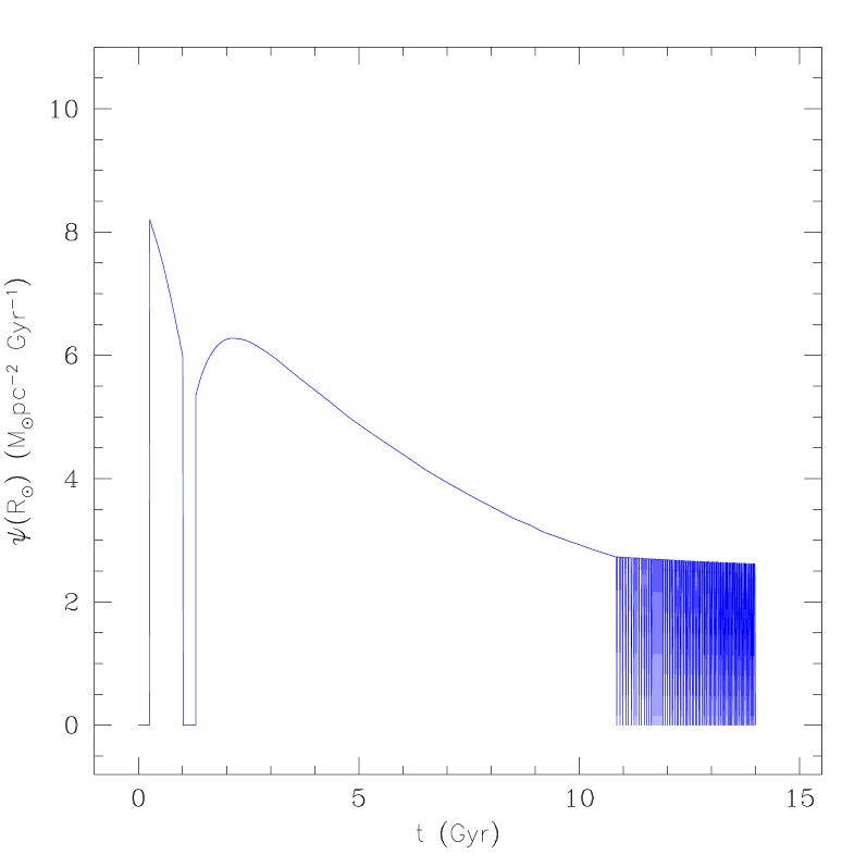
Figure 1: Predicted star formation rate in the halo-thick disk phase and in the thin disk phase during the evolution of the Milky Way. Notice that because of the existence of a threshold in the gas density the SFR halts in between the two major episodes of infall and oscillates in the last phases of the evolution of the disk. The models are from Chiappini et al. (2001).

6.3 Applications to the Local Disk

• The G-dwarf metallicity distribution is shown in Figure 2 where the data are compared with the predictions of the two infall model assuming a time scale for the formation of the local disk of 8 Gyr. (Chiappini et al. 1997; Boissier and Prantzos 1999; Chang et al. 1999; Chiappini et al. 2001).

  

  
  

  Figure 2: Observed and predicted G-dwarf metallicity distribution. The data are from Rocha-Pinto and Maciel (1996) and Hou et al. (1998). The model predictions (continuous line) are from Chiappini et al. (2001). The model assumes that the timescale for the disk formation in the solar neighbourhood is 8 Gyr.

• The relative abundance ratios as functions of the relative metallicity (relative to the Sun) [X/Fe] vs. [Fe/H], they are interpreted as due to the time-delay between Type Ia and II SNe. In fact, for the $\alpha$-elements the slowly declining [$\alpha$/Fe] ratio at low [ Fe/H] (halo phase) is normally interpreted as due to the pollution from massive stars, whereas the abrupt change in slope occurring at $\sim[Fe/H]=-1.0$ dex is due to the Type Ia SNe restoring the bulk of iron. From the [$\alpha$/Fe] vs. [Fe/H] diagram one can infer the timescale for the formation of the halo ($\tau_{h}\sim$ 1.5-2.0 Gyr, Matteucci and François, 1989; Chiappini et al. 1997), just by means of the age-[Fe/H] relationship, which indicates the time at which the metallicity of the turning point is reached. In Figure 3 we do not show the usual plot but [Fe/O] vs. [O/H] since in this plot are evident some features which do not appear in the classical diagram. In particular, the data show evidence for a gap around [O/H]= -0.3 dex, corresponding to [Fe/H] $\sim$ -1.0 dex (Gratton et al. 2000). This gap is well reproduced by the model which predicts a hiatus (no more than 1 Gyr) in the SFR between the end of the thick-disk phase and the beginning of the formation of the thin disk. This hiatus produces, in fact, a situation where O is no longer produced whereas Fe is produced, and this is revealed by the increase of [Fe/$\alpha$] at constant [$\alpha$/H]. This effect has been observed also for [Fe/Mg] vs. [Mg/H] by Furhmann (1998). The model shown in Figure 3 is a two-infall model with a threshold density for the star formation and is just the existence of such a threshold which produces the hiatus in the SFR, evident in Figure 1.

Figure 3: The [Fe/O] vs. [O/H] relation in the solar neighbourhood. The data are from Gratton et al.(2000) and the model (continuous line) from Chiappini et al.(2001). In this figure is evident the existence of a gap in the data at around [O/H]=-0.3 dex, corresponding to [Fe/H] $\sim$ -1.0 dex, which is also predicted by the model.

6.4 Applications to the whole disk

• Abundance Gradients are known to exist along the Galactic disk from data from various sources (HII regions, PNe, B stars). These data suggest that the gradient for oxygen is $\sim-0.07$ dex/kpc in the galoctocentric distance range 4-14 kpc. It is not yet clear if the slope is unique or if there is a change in slope as a function of the galactocentric distance. Similar gradients are found for N and Fe (see Matteucci 2001 and references therein).

• Gas Distribution. HI is roughly constant over a range of 4-10 kpc along the Galactic disk while $H_{2}$ follows the light distribution. No models can explain the two distributions. The total gas increases towards the center with a peak at 4-6 kpc.

• The SFR Distribution is obtained from various tracers (Lyman-$\alpha$ continuum, pulsars, SN remnants, molecular clouds) and shows that the SFR increases with decreasing galactocentric distance reaching a peak at 4-6 kpc in correspondence of the gas peak.

In order to fit gradients, SFR and gas one has to assume that the disk formed inside-out, in agreement with a previous suggestion by Larson (1976) and that the SFR should be a strongly varying function of the galactocentric distance. In Figure 4 is shown a comparison between an inside-out model and the abundance gradient, the gas, star and SFR distributions.

Figure 4: Comparison between data and model predictions from Chiappini et al. (2001) (continuous lines). In the first panel from the top we show the oxygen abundance gradient. In the second panel the variation of the $SFR/SFR_{\odot}$, in the third panel the gas distribution and in the fourth panel the distribution of stars along the Galactic disk.

6.5 The Role of Radial Flows in the evolution of the Galactic Disk

The gas infalling onto the disk can induce radial inflows by transferring angular momentum to the gas in the disk. Angular momentum transfer can be due to the gas viscosity in the disk and induce inflows in the inner parts of the disk and outflows in the outer parts. All viscous models suggest that metallicity gradients can be steepened by radial (in)flows, especially if an outer star formation cut-off is assumed (Clarke 1989; Yoshii & Sommer-Larsen 1989). All models agree that the velocity of radial (in)flows should be low ($v<2$ km/sec). Observationally is not clear if these radial flows exist. Edmunds & Greenhow (1995), by means of analytical models of galactic chemical evolution concluded that there is no simple one-way effect of radial flows on abundance gradients. Portinari & Chiosi (2000) suggested that radial inflows may represent a possible explanation of the peak of the gas at 4-6 kpc. In our opinion radial flows, if they exist, are never the main cause for the formation of abundance gradients.

6.6 The Role of the IMF in the evolution of the Galactic Disk

Abundance gradients, in principle can be obtained by a variation of the IMF along the disk. One can assume either that more massive stars form in external regions or the contrary, that more low mass stars form in external regions. It has been shown convincingly that neither of the two options work (Carigi 1996; Chiappini et al. 2000), and that there is no evidence in favor of such variations along the Galactic disk. Therefore, we can exclude the variation of the IMF as the main cause of abundance gradients and conclude that the best agreement with the observed properties of the Galactic disk is obtained by assuming a constant IMF.

6.7 Scenarios for Bulge Formation

Various scenarios have been proposed insofar for the formation of the Galactic bulge but only one seems to reproduce the observed abundance pattern. Here I recall the main scenarios:

• Accretion of extant stellar systems which eventually settle in the center of the Galaxy.

• Accumulation of gas at the center of the Galaxy and subsequent evolution with either fast or slow star formation.

• Accumulation either rapid or slow of metal enriched gas from the halo or thick disk in the Galaxy center.

• Formation occurs out of inflow of metal enriched gas from the thin-disk.

The metallicity distribution of stars in the bulge as well as the [$\alpha$/Fe] vs. [Fe/H] relations help in selecting the most probable scenario and suggest that a fast accumulation of gas in the Galactic center accompanied by fast star formation is the best scenario. In this framework, the bulge must have formed contemporarily to the inner halo on a similar timescale. In Figures 5 and 6 we show some model predictions compared with the metallicity distribution of bulge stars and the predicted [$\alpha$/Fe] vs. [Fe/H] ratios for the bulge together with the predictions for the solar neighbourhood. The model for the bulge presented in the two figures (Matteucci, Romano & Molaro, 1999) assumes a much stronger star formation rate than in the solar neighbourhood (by a factor of 10) with the same nucleosynthesis prescriptions and a timescale for bulge formation of 0.5 Gyr as opposed to 8 Gyr in the solar vicinity. In Figure 5 it is evident that the best model to reproduce the stellar metallicity distribution requires a Salpeter (1955) IMF which is sligthly flatter than that used for the solar neighbourhood (Scalo, 1986). The predicted [$\alpha$/Fe] ratios in Figure 6 indicate that the bulge stars should show overabundances of $\alpha$-elements for most of the [Fe/H] range, as it seems also suggested by observations (Mc William & Rich, 1994; Barbuy, 1999). This is a consequence of the time-delay between Type Ia and II SNe, coupled with a very fast evolution in the bulge as compared to the solar vicinity. In fact, in this case high values of [Fe/H] are reached in the gas before a substantial number of SNe Ia has the time to restore the bulk of iron. The contrary occurs in a system with lower star formation than in the solar neighbourhood, such as the external regions of the disk and irregular galaxies. In these systems we expect that the overabundance of $\alpha$-elements relative to Fe is maintained only for a short interval of [Fe/H] (see Pagel, 1997: Matteucci 2001).

Figure 5: Comparison between data (dotted lines) and model predictions for the metallicity distribution of bulge stars. The data are from McWilliam & Rich (1994) and the models (continuous lines) from Matteucci et al. (1999). Each panel corresponds to a model with a different IMF slope, as indicated.

Figure 6: Predicted [$\alpha$/Fe] vs. [Fe/H] relations for the bulge (continuous lines) and for the solar neighbourhood (dotted lines). The models are from Matteucci et al. (1999).

7 Disks of Other Spirals

Abundance gradients

Abundance gradients in dex/kpc are known to exist also in the disk of other spirals showing that they are steeper in smaller disks, but this correlation disappears if the gradients are expressed in units of dex/scalelength, thus indicating the existence of a universal slope per unit scalelength (e.g. Garnett, 1998). Another remarkable characteristic about abundance gradients in other spirals is that they appear to be flatter in galaxies with central bars, suggesting that the dynamical effect of the bar can influence the evolution of the disk.

The SFR

The SFR is measured mainly from $H_{\alpha}$ emission (Kennicutt, 1998) and implies a correlation with the total surface gas density (HI+$H_{2}$) as discussed in section 2.1.

Gas distributions

Gas distributions, especially the HI distribution is known for a fair sample of spirals. There are indications of differences between field and cluster spirals (e.g. Skillman et al. 1996).

Integrated colors

Studies of integrated colors of spiral disks reflect the observed abundance gradients and are well reproduced by an inside-out formation of disks similar to what assumed for the Milky Way (Josey & Arimoto 1992; Jimenez et al. 1998; Prantzos & Boissier 2000).

8 Conclusions on the Milky Way and other spirals

The comparison between observations and models for the Milky Way suggests that:

• The disk of the Galaxy formed mostly by infall of primordial or very metal poor gas accumulating faster in the inner than in the outer regions (inside-out scenario, i.e. $\tau_{D}(R)$ decreases with decreasing R).

• In the framework of the inside-out scenario, the SFR should be a strongly varying function of the galactocentric distance. In particular, it should either depend on the total surface mass density (feed-back mechanism) or on the angular circular velocity of gas. Both formulations for the SFR are supported by observations. Under the assumption of a strongly varying SFR, the observed abundance gradients can be nicely reproduced.

• Radial flows probably are not the main cause of gradients but can help in reproducing the gas profile.

• A constant IMF (in time and space) should be preferred, since variable IMFs have been tested and they cannot reproduce all of the observational constraints of the solar neighbourhood and the whole disk at the same time.

• The properties of the disks of other spirals also indicate an inside-out disk formation.

• In the framework of semi-analytical models of galaxy formation (Mo, Mao & White, 1998), the evolution of galaxy disks can be described by means of scaling laws calibrated on the Galaxy with $V_{c}$ and $\lambda$ as parameters (Jimenez et al. 1998; Prantzos & Boissier, 2000), where $V_{c}$ is a measure of the mass of the dark halo and $\lambda$ is a measure of the specific angular momentum of the halo.

• Dynamical processes such as the formation of a central bar can influence the evolution of disks and deserve more attention in the future.

• Abundance ratios (e.g. [$\alpha$/Fe]) in stars al large galactocentric distances can give us a clue to interpret the formation of the disk and the halo (inside-out or outside-in). In fact, in a typical inside-out scenario we predict that the [$\alpha$/Fe] ratios would decrease with galactocentric distance, due to the weaker and sometimes intermittent SF regime, whereas in an outside-in scenario we would expect the contrary due to the faster evolution of the more external region which quickly consume the gas before Type Ia SNe have time to restore the bulk of Fe.

• The predictions of chemical evolution models can be tested in a cosmological context to study the galaxy surface brightness and size evolution as a function of redshift. Roche et al. (1998) have already done that and suggested that a size and luminosity evolution, as suggested by the inside-out scenario fits better the observations.

• Inside-out formation of the Galaxy is suggested also by the fact that the globular clusters of the inner halo are coeval ($\Delta t\sim 0.5$ Gyr, Rosenberg et al. 1999), whereas the age difference seems to increase in the outer halo.

• The metallicity distribution of stars in the Bulge as well as the observed [$\alpha$/Fe] ratios suggest a very fast formation of the Bulge ($\sim$ 0.5-0.8 Gyr), due a the very fast SFR, as predicted by succesfull chemical evolution models and by Elmegreen (1999).

9 Elliptical Galaxies

Elliptical galaxies are mainly found in galaxy clusters, they show a large range of luminosities and masses and are made by stars as old as those in globular clusters. No cold gas is observed in these galaxies but hot X-ray gas halos are present. Because of their large masses and metal content they are probably the most important factories of metals in the universe.

9.1 Observational properties

Here I recall the main observational features of elliptical galaxies:

• The existence of Color-Magnitude and color - velocity dispersion ($\sigma_{o}$) relations (colors become redder with increasing luminosity and mass; e.g. Bower et al. 1992) is interpreted as a metallicity effect, namely as the fact that the metallicity decreases outwards similarly to what happens in spiral disks.

• The existence of a $Mg_{2}$–$\sigma_{o}$ (where $Mg_{2}$ is a metallicity index) relation reinforces the previous point (Bender et al. 1993; Bernardi et al. 1998; Colless et al. 1999; Kuntschner et al. 2001).

• Inside ellipticals, $Mg_{2}$ correlates also with the escape velocity $v_{esc}$, as first shown by Franx & Illingworth (1990), indicating that the magnesium index is larger where the escape velocity is larger.

• $M/L_{B}$ increases by a factor of $\sim 3$ from faint to bright ellipticals implying a tilt of the fundamental plane of ellipticals (Bender et al. 1992). The fundamental plane is the particular plane occupied by these galaxies in the space defined by the stellar velocity dispersion, the effective radius and the surface brigthness.

• Abundance gradients inside ellipticals have been measured by means of metallicity indices such as $Mg_{2}$ and $<Fe>$ (Carollo et al. 1993; Davies et al. 1993; Kobayashi & Arimoto 1999). These gradients correspond roughly to a gradient in [Fe/H] of the stellar component of $\Delta[Fe/H]/\Delta logr\sim-0.3$.

  The average metallicity of the stellar component in ellipticals is $<[Fe/H]>_{*}\sim-0.3$dex (from -0.8 to +0.3).

• By comparing synthetic metallicity indices with the observed ones some authors (Worthey et al. 1992; Weiss et al. 1995; Kuntschner et al. 2001) have suggested that the average stellar $<[Mg/Fe]>_{*}$ is larger than zero (from 0.05 to + 0.3 dex) in nuclei of giant ellipticals. Moreover, there is indication that $<[Mg/Fe]>_{*}$ increases with increasing $\sigma_{o}$ ($M_{gal}$) and luminosity (Worthey et al. 1992; Jorgensen 1999; Kuntschner et al. 2001).

  In particular the relation found by Kuntschner et al. (2001) is: [Mg/Fe]=$0.30(\pm 0.06)log\sigma_{o}-0.52(\pm 0.15)$.

9.2 Formation of Ellipticals

Several mechanisms have been suggested for the formation and evolution of elliptical galaxies, in particular:

• Early monolithic collapse of a gas cloud or early merging of lumps of gas where dissipation plays a fundamental role (Larson 1974; Arimoto & Yoshii 1987; Matteucci & Tornambè 1987 ). In this scenario the star formation stops soon after a galactic wind develops and the galaxy evolves passively since then.

• Bursts of star formation in merging subsystems made of gas (Tinsley & Larson 1979). In this picture star formation stops after the last burst and gas is lost via stripping or wind.

• Early merging of lumps containing gas and stars in which some dissipation is present (Bender et al. 1993).

• Merging of early formed stellar systems in a wide redshift range and preferentially at late epochs (Kauffmann et al. 1993). A burst of star formation can occur during the major merging where $\sim 30\%$ of the stars can be formed (Kauffmann 1996).

The main difference between the monolithic collapse scenario and the hierarchical merging relies in the time of galaxy formation, occurring quite early in the former scenario and continuously in the latter scenario. As we will see, there are arguments either in favour of the monolithic or the hierarchical scenario.

9.3 Formation of Ellipticals at low z

Here I recall some of the main arguments in favor of the formation of ellipticals at low redshifts:

• Relative large values of the $H_{\beta}$ index measured in a sample of nearby ellipticals which could indicate prolonged star formation activity up to 2 Gyr ago (Gonzalez 1993; Trager et al. 1998).

• The tight relations in the fundamental plane are due to a conspiracy of age and metallicity in the sense that it should exist an age-metallicity anticorrelation implying that the more metal rich galaxies are also younger (Ferreras et al. 1999; Trager et al. 2000).

• The apparent paucity of high luminosity ellipticals at $z\sim 1$ compared to now claimed by a series of authors (Kauffmann et al. 1993; Zepf, 1997; Menanteau et al. 1999).

9.4 Formation of Ellipticals at high z

Here I recall the arguments in favor of a formation of ellipticals at high redshift:

• The tightness of the color-central velocity dispersion relation found for Virgo and Coma galaxies (Bower et al. 1992). If the formation of ellipticals were a continuous process we should expect a much larger spread in the galaxy colors for a given central velocity dispersion. In particular, the argument goes like that: from the observed color scatter one can derive $t_{H}-t_{F}\sim 2$Gyr (where $t_{H}$ is the Hubble time and $t_{F}$ the time of galaxy formation). If $t_{H}=15$ Gyr then the youngest ellipticals must have formed $\sim 13$ Gyr ago at $z\geq 2$ (Renzini, 1994).

• The thinness of the fundamental plane for ellipticals in the same two clusters, in particular the $M/L$ vs. $M$ relation (Renzini & Ciotti 1993).

• The tightness of the color-magnitude relation for ellipticals in clusters up to $z\sim 1$ (Kodama et al. 1998; Stanford et al. 1998)

• The modest passive evolution measured for cluster ellipticals at intermediate redshift (van Dokkum & Franx 1996; Bender et al. 1996).

• Lyman-break galaxies at $z\geq 3$ where the SFR$\sim 50-100M_{\odot}yr^{-1}$ could be the young ellipticals (Steidel et al. 1996; 1998).

• The strongly evolving population of Luminous Infrared Galaxies suggesting that they are progenitors of massive spheroidals (Blain et al. 1999; Elbaz et al. 1999).

9.5 Models for ellipticals based on galactic winds

Monolithic models assume that ellipticals suffer a strong star formation and quickly produce galactic winds when the energy from SNe injected into the ISM equates the potential energy of the gas. Then, star formation is assumed to halt after the development of a galactic wind. In this framework, the evolution of ellipticals crucially depends on the time at which a galactic wind occurs, $t_{GW}$. For this reason, it is extremely important to understand the SN feedback and star formation process. The condition for the onset of a wind can be written as:

$$(E_{th})_{ISM}\geq E_{Bgas}$$ (9.53)

The thermal energy of gas due to SNe and stellar wind heating is:

$$(E_{th})_{ISM}=E_{th_{SN}}+E_{th_{w}}$$ (9.54)

with

$$E_{th_{SN}}=\int^{t}_{0}{\epsilon_{SN}R_{SN}(t^{`})dt^{`}}$$ (9.55)

and

$$E_{th_{w}}=\int^{t}_{0}\int^{100}_{12}{\varphi(m)\psi(t^{`})\epsilon_{w}dmdt^{`}}$$ (9.56)

for the contribution from SNe and stellar winds, respectively. The quantity $R_{SN}$ represents the SN rate (II and Ia). The quantities $\epsilon_{SN}=\eta_{SN}\epsilon_{o}$ with $\epsilon_{o}=10^{51}$erg where $\epsilon_{o}$ is the typical SN blast wave energy , and $\epsilon_{w}=\eta_{w}E_{w}$ with $E_{w}=10^{49}$erg (typical energy injected by a $20M_{\odot}$ star taken as representative), are the efficiencies for the energy transfer from SNe II and Ia into the ISM. These efficiencies, $\eta_{w}$ and $\eta_{SN}$, can be assumed as free parameters or be calculated from the results of the evolution of a SN remnant in the ISM and the evolution of stellar winds. The SN feedback is, in fact, a crucial parameter. The formulation of Cox (1972) for the efficiency of energy injection from SNe derives from following the evolution of the shock wave produced by the explosion into an ISM with constant density:

$$\epsilon_{SN}=0.72\epsilon_{o}\,\,erg$$ (9.57)

for $t_{SN}\leq t_{c}=5.710^{4}\epsilon_{o}^{4/17}n_{o}^{-9/17}$ years, where $t_{c}$ is the cooling time, and $t_{SN}$ is the time elapsed from the SN explosion, and:

$$\epsilon_{SN}=2.2\epsilon_{o}(t_{SN}/t_{c})^{-0.62}\,\,erg$$ (9.58)

for $t_{SN}>t_{c}$.

With these prescriptions only few $\%$ of $\epsilon_{o}$ are deposited into the ISM (see Bradamante et al. 1998). However, multiple SN explosion should change the situation. Unfortunately, very few calculations of this type are available. An important point to consider is also that SNe Ia, which explode after Type II SNe, should provide more energy into the ISM than Type II SNe since they explode in an already formed cavity (see Recchi, Matteucci & D’Ercole, 2001).

The total mass of the galaxy is expressed as $M_{tot}(t)=M_{*}(t)+M_{gas}(t)+M_{dark}(t)$ with $M_{L}(t)=M_{*}(t)+M_{gas}(t)$ and the binding energy of gas is:

$$E_{Bgas}(t)=W_{L}(t)+W_{LD}(t)$$ (9.59)

and:

$$W_{L}(t)=-0.5G{M_{gas}(t)M_{L}(t)\over r_{L}}$$ (9.60)

represents the potential well due to the luminous matter, whereas:

$$W_{LD}(t)=-Gw_{LD}{M_{gas}(t)M_{dark}\over r_{L}}$$ (9.61)

is the potential well due to the interaction between dark and luminous matter, where $w_{LD}\sim{1\over 2\pi}S(1+1.37S)$ with $S=r_{L}/r_{D}$(Bertin et al. 1992).

The SFR is usually assumed to be:

$$SFR=\nu M_{gas}$$ (9.62)

where $\nu\propto M_{L}^{-\gamma}$ ($\gamma$ =-0.11, Arimoto & Yoshii 1987), owing to the fact that the star formation efficiency is just the inverse of the timescale for star formation:

$$\nu=\tau_{SF}^{-1}$$ (9.63)

and that:

$$\tau_{SF}\propto\tau_{coll}\propto\tau_{ff}$$ (9.64)

with $\tau_{coll}$ and $\tau_{ff}$ being the collapse and the free-fall timescale, respectively. Since dynamical timescales are longer for more massive galaxies, the efficiency of star formation should decrease with galactic mass. The efficiency $\nu$ coupled with the increase of the potential well as $M_{L}$ increases leads to the fact that more massive galaxies form stars for a longer period before suffering a galactic wind. This fact has been invoked for explaining the observed mass-metallicity relation (Larson, 1974). However, this is at variance with the observed [Mg/Fe] vs. $\sigma_{o}$ relation, since in this scenario the more massive ellipticals should show the lowest [Mg/Fe].

9.6 Failure of Larson’s Model

There are different ways of obtaining that $[Mg/Fe]$ in the stellar component increases when the galactic mass $M_{L}$ increases. These ways are:

• Different timescales for star formation (Worthey et al. 1992) in the sense that star formation should be more efficient in more massive galaxies ($\nu\propto M_{L}^{\gamma}$). In this case, the situation could be such that a galactic wind occurs earlier in more massive systems, the inverse wind scenario (Matteucci 1994).

• A variable IMF from galaxy to galaxy favoring more massive stars (Mg producers) in more massive galaxies (Worthey et al. 1992; Matteucci, 1994).

• Different amounts and/or concentrations of dark matter as functions of $M_{L}$ In particular, less dark matter should be present in the most massive systems (Matteucci, Ponzone & Gibson, 1998). As a consequence of this, again galactic winds occur earlier in more massive objects.

• A selective loss of metals: more massive systems loose more Fe relative to $\alpha$-elements than less massive ones (Worthey et al. 1992).

As mentioned before, Matteucci (1994) proposed a model that she called inverse wind model, where the efficiency of star formation is an increasing function of galactic mass, thus implying a shorter period of star formation in massive ellipticals. In fact, the efficiency of star formation is chosen in such a way that in massive ellipticals the galactic wind occurs before than in less massive ones. This produces the increase of the [Mg/Fe] ratio as a function of galactic mass. This approach bears a resemblance with the merging scenario of Tinsley & Larson (1979) where the efficiency of star formation was assumed to increase with the total mass of the system. In the inverse wind model a very massive elliptical of $M_{L}=10^{12}M_{\odot}$ starts developing a wind before 1 Gyr from the beginning of star formation, whereas a small ellipticals form stars for a longer period. As a result, the average $<[Mg/Fe]>_{*}$ is larger in massive than in small ellipticals. The same effect can be obtained by varying the IMF in such a way that more massive ellipticals tend to form more massive stars. It is worth noting that this second hypothesis could also explain the tilt of the fundamental plane in $M/L_{B}$. On the other hand, the hypothesis of the variable dark matter does not produce relevant effects, as shown by Matteucci et al. (1998). The only assumption which has not been tested quantitatively is the selective loss of metals. The main problem with all of these alternatives is, in any case, the lack of a good physical justification depending on the poorly known processes of star formation and SN feeback, and in the future some effort should be devoted to these fields.

It is worth noting that the hierarchical clustering scenario for galaxy formation cannot produce a solution to the observed [Mg/Fe] trend in ellipticals. In fact, it rather predicts the contrary, as shown by Thomas (1999) and Thomas et al. (2002). In fact, in the hierachical clustering the period of star formation in the most massive ellipticals is predicted to be the longest thus favoring low [Mg/Fe] ratios in massive objects, as shown in Figure 7.

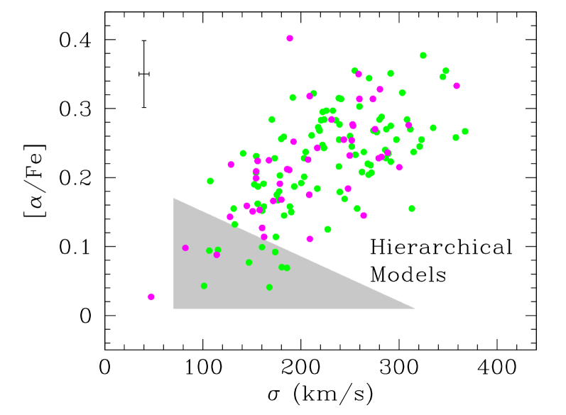
Figure 7: Predicted [$\alpha$/Fe] vs. velocity dispersion for elliptical galaxies. Data are compared with predictions obtained by adopting the star formation history assumed in hierarchical clustering models for galaxy formation.The models and the figure are from Thomas et al. (2002).

Figure 8: Predicted and observed color gradients for some field elliptical galaxies. From Menanteau et al. (2001).Figure shows from left to right: $I_{814}$-band surface brightness map, $V_{606}$-$I_{814}$ color pixel map and $V_{606}$-$I_{814}(r)$ color gradient. Open circles represent observed gradients while solid lines are the model predictions obtained by means of the Martinelli et al. (1998) model.

9.7 Averaged Stellar Metallicities

The metallicity in elliptical galaxies always refers to the metal content of the stars, in particular of the stellar population dominating in the visual light. For this reason we should define the average stellar metallicity. In particular, the average metallicity of a composite stellar population averaged on the mass is:

$$<X_{i}>_{m}={1\over S_{1}}\int^{S_{1}}_{0}{X_{i}(S)dS}$$ (9.65)

where $1$ refers to the specific time $t_{1}$ and $S_{1}$ is the total mass of stars ever born. This is the real average metallicity but in order to compare models and observations it is more appropriate to define the metallicity averaged on the visual light. In particular, the average metallicity of a composite stellar population averaged on the light is:

$$<X_{i}>_{L}={\sum_{ij}{n_{ij}X_{i}L_{Vj}}\over\sum_{ij}{n_{ij}L_{Vj}}}$$ (9.66)

where $n_{ij}$ is the number of stars in the abundance interval $X_{i}$ and luminosity interval $L_{Vj}$.

It is worth noting that $<X_{i}>_{m}$ is larger than $<X_{i}>_{L}$ for galaxies with $M_{L}<10^{9}M_{\odot}$, since metal poor giants dominate the visual light whereas they are similar for larger masses (Yoshii & Arimoto 1987).

9.8 Multi-Zone Models

There are two multi-zone chemical evolution models for ellipticals available in the literature (Martinelli et al. 1998; Tantalo et al. 1998). Martinelli et al. (1998) assumed that the elliptical galaxy is divided in several concentric shells of thickness $\Delta R_{i}$. The binding energy of the gas in each shell is computed after assuming a dark matter halo as described before. The model predicts that a galactic wind develops first in the external regions and then gradually in the more internal ones in agreement with the observed $Mg_{2}$ vs. $v_{esc}$ relation. As a consequence of this, the star formation lasts for a shorter time in the external regions with the consequence that an abundance gradient is created in agreement with observations. This model also predicts that we should observe higher [Mg/Fe] ratios at larger galactocentric distances, the contrary of what should happens in the disks of spirals. In this case, we can speak of outside-in formation. Unfortunately, the available data inside galaxies do not allow yet to observe such an effect. It is worth noting that this model can reproduce very well the observed color gradients in ellipticals, as shown in Figure 8.

10 Conclusions on Ellipticals

The main conclusions that we can draw from comparing theoretical models and observations for ellipticals can be summarized as follows:

• In order to explain the observed $<[Mg/Fe]>_{*}>0$ in giant ellipticals the dominant stellar population should have formed on a time scale no longer than 3-5 $\cdot 10^{8}$ yr, which corresponds to the time at which the SNe Ia rate reaches a maximum in these systems with strong star formation.

• Uncertainties in the stellar yields of Fe and Mg from different authors can change the value of the [Mg/Fe] ratio but do not affect the conclusion above.

• This observational finding argues against a hierarchical clustering formation scenario and favors the fact that ellipticals, especially those in clusters, are mostly old systems (see also Menanteau et al. 2001).

• The increase of the [Mg/Fe] ratio with galactic mass suggests either that more massive ellipticals are older systems or that the IMF is not constant among ellipticals or both.

• Abundance gradients in ellipticals can be produced by biased winds and this would imply that [Mg/Fe] increases with increasing galactocentric distance.

• Better calibrations for metallicity indices are necessary, especially taking into account non-solar ratios in stellar tracks, before drawing firm conclusions.

11 Evolution of Dwarf Galaxies

Dwarf Irregular (DIG) and Blue Compact (BCG) galaxies are very interesting objects for studying galaxy evolution since they are relatively unevolved objects (see Kunth & Östlin, 2000, for a recent exhaustive review). In bottom-up cosmological scenarios they should be the first self- gravitating systems to form, thus they could also be important contributors to the population of systems giving rise to QSO-absorption lines at high redshift (DLAs). In general, they are rather simple objects with low metallicity and large gas content, suggesting that they are either young or have undergone discontinuous star formation activity (bursts). An important characteristic of these systems is that they show a distinctive spread in their physical properties, such as chemical abundances versus fraction of gas. Matteucci and Chiosi (1983) were among the first in studying the chemical evolution of dwarf galaxies. They adopted analytical models as those described in section 3 and showed that closed-box models cannot account for the Z-log$\mu$ distribution even if the number of bursts varies from galaxy to galaxy, and suggested possible solutions to explain the observed spread:

• a. different IMFs

• b. different amounts of galactic wind

• c. different amounts of infall

Later on, Matteucci and Tosi (1985) presented a numerical model where galactic winds powered by SNe were taken into account. They concluded that different wind rates from galaxy to galaxy could explain the observed spread in O,N vs. log$\mu$ but not the spread in the N/O vs. O/H diagram, suggesting that additional processes could have contributed to that. For example, different amounts of primary N from galaxy to galaxy. Kumai and Tosa (1992) suggested that different fractions of dark matter in different objects could explain the observed spread in the Z-log$\mu$ diagram. Pilyugin (1993) forwarded the idea that the spread in the properties of these galaxies (i.e. He/H vs. O/H and N/O vs. O/H) are due to self-pollution of the HII regions coupled with “enriched” or “differential” galactic winds. Differential winds should carry out of the galaxy certain elements more than others, for example the metals ejected by SN II should be favored. In more recent models (Marconi et al. 1994; Bradamante et al. 1998), the novelty was the contribution to the chemical enrichment of SNe of different type (II,Ia and Ib) together with differential winds. In these papers the assumption was made that the products of SN II are lost more easily than the products of stars ending as WDs, such as C and N. Larsen et al. (2001) studied the chemical evolution of gas rich dwarf galaxies and concluded that primary N production from massive stars is not necessary to reproduce the N/O vs O/H and that the spread in this relation is likely to be due to the time-delay effect in the production of N relative to the production of O. In fact, in a starbursting regime when the starburst fades the elements produced by Type II SNe are no more produced whereas the elements produced on long timescales by single stars and Type Ia SNe are still produced. This causes the typical saw-tooth behaviour (see Figure 9). Therefore, the spread can be due to the fact that some objects are observed at different stages of the burst/interburts regime. They also concluded that ordinary winds are better than enriched ones in reproducing the properties of these objects. The existence of a luminosity-metallicity relation (although with spread) can be an indication for galactic winds acting more efficiently in low mass than in high mass high potential well objects.

11.1 Evidences for Galactic Winds

Meurer et al (1992), Papaderos et al. (1994), Lequeux et al. (1995) and Marlowe et al. (1995) all suggested the existence of galactic winds in dwarf starbursting galaxies. The evidence is gathered by the indication of outflowing material travelling at a speed larger than the assumed mass of the objects. Papaderos et al. estimated a galactic wind flowing at a velocity of 1320 Km/sec for VIIZw403. The escape velocity estimated for this galaxy being 50 Km/sec. Lequeux et al.(1995) suggested a galactic wind in Haro2=MKn33 flowing at a velocity of $\simeq 200Km/sec$. Martin (1996;1998) found supershells in 12 dwarfs including IZw18 and concluded that they imply an outflow which in some cases can become a wind (namely the material is lost from the galaxy).

Recent chemo-dynamical simulations for one instantaneous starburst also suggest the possibiliy of galactic winds and that these winds are metal enriched (MacLow & Ferrara 1999; Recchi et al. 2001).

11.2 Results for BCG from chemical models

Purely chemical models (no dynamics) have been computed by several authors by varying the number of bursts, the time of occurrence of bursts, $t_{burst}$, the star formation efficiency, the type of galactic wind, the IMF and the nucleosynthesis prescriptions (Marconi et al. 1994; Kunth et al.1995; Bradamante et al.1998). The main conclusions of these papers can be summarized as follows:

• The number of bursts should be $N_{bursts}\leq 10$, the star formation efficiency should vary from 0.1 to 0.7 $Gyr^{-1}$ for either Salpeter or Scalo (1986) IMF but Salpeter IMF is favored.

• Enriched winds, carrying out material at a rate proportional to the star formation rate, seem to be preferred (but see Larsen et al. 2001). The observed scatter in the observational properties can be due either to the winds or to the delay in the production of different elements.

• If the burst duration is relatively short (no more than 100 Myr), SNe II dominate the chemical evolution and energetics of starburst galaxies, while stellar winds seem to be negligible after the onset of SNe II.

• The [O/Fe] ratios tend to be overabundant due to the predominance of Type II SNe during the bursts. Models with a large number of bursts $N_{burst}$=10 - 15 can give negative [O/Fe].

Figure 9: The log(N/O) vs. 12 +log(O/H) for a sample of BCG. The data are from Recchi (2002). Overimposed are three models with a single burst of star formation and different star formation efficiency. In particular, the dotted line corresponds to an efficiency $\nu=1Gyr^{-1}$, the continuous line to $\nu=2.5Gyr^{-1}$ and the dashed line to $\nu=5Gyr^{-1}$. The burst duration is 100 Myr. As one can see, the saw-tooth behaviour typical of a bursting mode of star fotmation is evident.

Figure 10: Chemo-dynamical simulation of an instantaneous starburst from Recchi et al. (2001). The development of a galactic wind is evident along the z-axis, since the assumed configuration is flattened.The age of the burst is indicated in Myr.

11.3 Results from chemo-dynamical models

Recent chemo-dynamical models (Recchi et al. 2001;2002) assuming an instantaneous starburst but following in great detail the evolution of several chemical elements (H, He, C, N, O, Mg, Si and Fe) and adopting an efficiency for SN II energy transfer $\eta_{SNII}$=0.003 and for SN Ia $\eta_{SNIa}$=1.0, suggest that the starburst triggers indeed a galactic wind (see Figure 10). In particular, the metals leave the galaxy more easily than the unprocessed gas and among the metals the SN Ia ejecta leave the galaxy more easily than the SN II ejecta. This is due to the assumed efficiencies for energy transfer for the two types of SNe. This assumption is in turn based on the fact that Type Ia SNe explode in an already heated and rarified medium (thanks to the Type II SNe which explode first) and therefore can transfer all of their energy into the ISM. As a consequence of this type of evolution the following conclusions can be drawn:

• A selective loss of metals seems to occur in dwarf gas-rich galaxies.

• As a consequence of the selective winds, the [$\alpha$/Fe] ratios inside the galaxy are predicted to be larger than the [$\alpha$/Fe] ratios outside the galaxy. In fact, the products of SNe Ia are lost more efficiently than those of SN II.

• At variance with previous studies, most of the metals are already in the cold gas phase after 8-10 Myr owing to the fact that the superbubble does not break immediately (the SNe II inject only a fraction of their initial blast wave energy into the ISM) and thermal conduction can act efficiently.

• The model well reproduces the properties of IZw18 (the most metal poor galaxy known locally) if two bursts are assumed and are separated by 300 Myr interval.

11.4 Dwarf galaxies and DLA Systems

Finally, before concluding this section, we would like to draw the attention upon the fact that there are similarities between BCG, DIG and DLAs or more in general between DLAs and systems with a low level of star formation.

The nature of DLA systems is under debate and the abundance ratios measured there can be used as a diagnostic to infer their nature and age. Matteucci et al. (1997) suggested that some DLA showing high N/O ratio could be BCG suffering selective winds. In this respect, the similarity between DLAs and IZw18 may suggest that IZw18 is a survivor proto-galaxy which has just started forming stars. If this is true, dwarf irregular galaxies should be born at any time during the age of the universe, unlike elliptical galaxies which appear to have formed a long time ago and in a short time interval (see section 9).

Figure 11: Redshift evolution of [Zn/H] for high surface brightness spirals (HSB) (bottom panels) and low surface brightness spirals (LSB) (upper panels) for different galactocentric distances in the disk. a) The evolution in metallicity of LSB formed at z=4 fits well the DLA values measured by Pettini et al. (1999).b) If LSB disks formed late, however, then they do not fit the data. c) Conversely, HSB disks that formed at z=4 become metal rich too quickly to explain the observations; d) only if there is a continuously forming population of HSB disks between z=4 and z=1 then they can account for the metallicities of the DLAs.

Plots of [$\alpha$/Fe] vs. [Fe/H] and plots of [$\alpha$/Fe] vs. redshift should be used to infer the nature and the age of these objects, when compared with chemical evolution predictions.

The observed abundance ratios seem to indicate that DLAs show almost solar [$\alpha$/Fe] ratios at low [Fe/H] (Pettini et al. 1999; Centurion et al. 2000). This is an indication that they are objects where the star formation proceeded slowly and that they have probably started to form stars long before the redshift at which we observe them. This could indicate that we are looking at the external regions of disks or at dwarf starbursting systems in the interburst phases (see Figure 11). However, more data are necessary to assess this point. One common problem related to the measurement of the abundances in DLAs is that some elements are dust depleted such as Si and Fe and therefore one should try to observe non-refractory elements such as N, O, S and Zn. One should also remember that Si and Ca do not strongly behave as $\alpha$-elements since they are produced in a non-negligible way in SNe Ia.

12 Chemical Enrichment of the ICM

After having discussed the chemical evolution of galaxies it is important to conclude by studying how the evolution of galaxies can affect the chemical enrichment of the intracluster (ICM) and intergalactic medium. In the past years a great deal of work has been presented on the subject. The first work on chemical enrichment of the ICM was by Gunn & Gott (1972), Larson & Dinerstein (1975), Vigroux (1977), Himmes & Biermann (1988). In the following years, Matteucci & Vettolani (1988) started a more detailed approach to the problem followed by David et al. (1991), Arnaud et al. (1992), Renzini et al. (1993), and many others. The majority of these papers assumed that galactic winds (mainly from ellipticals) are responsible for the ICM chemical enrichment. Alternatively, the abundances in the ICM could be due to ram pressure stripping (Himmes & Biermann 1988) or to pre-galactic Population III stars (White & Rees 1978).

12.1 Models for the ICM

Here we will describe briefly the metodology developed by Matteucci & Vettolani (1988) (hereafter MV88). Starting from SN driven galactic wind models for ellipticals (see section 9) they computed the ejected masses vs. final baryonic total galactic masses for galaxies of different initial luminous masses (from $10^{9}$ to $10^{12}M_{\odot}$):

$$M_{i}^{ej}=E_{i}M_{f}^{\beta_{i}},$$ (12.67)

where $i$ refers to either a single chemical element or the total gas. Then, they integrated $M_{i}^{ej}$ over the cluster mass function obtained from the Schechter (1986) luminosity function (LF) by assuming that only E and S0 galaxies contribute to the chemical enrichment. This assumption was later confirmed by data of Arnaud et al. (1992). The total masses ejected into the ICM in the form of single species $i$ and total gas are:

$$M_{i,clus}^{ej}(>M_{f})=E_{i}fn^{*}(h^{2}k)^{\beta_{i}}10^{-0.4\beta_{i}(M^{*}-5.48)}\cdot\Gamma[(\alpha+1+\beta_{i}),(M_{f}^{*}h^{2}/k)10^{-0.4(M_{B}^{*}-5.48)}]$$ (12.68)

where $\alpha$ is the slope of the LF, $f$ is fraction of ellipticals plus S0, $M^{*}$ is the mass at the “break” of the LF and $M_{B}^{*}$ is the magnitude at the break.

12.2 MV88 Results

MV88 considered 4 galaxy clusters: Perseus, A2199, Coma and Virgo for which $f$, $n^{*}$, $M^{*}$, $M_{Fe}$ and $M_{gas}$ were known. In Table 1 we show the results they obtained for the 4 clusters concerning the total masses ejected by all galaxies in the clusters in the form of total gas and Fe, compared with the observed ones. It is immediate to see from Table 1 that their model could reproduce well the total amount of Fe but they failed in reproducing the total gas mass. However, this is not a failure of the model but the indication that most of the gas in clusters has a primordial origin, namely has never been processed inside stars. The same conclusion was reached later by David et al. (1991) and Renzini et al. (1993) among others, but see Chiosi (2000).

Table 1. Predicted and observed quantities

Cluster	$(M_{Fe})_{pred}$	$(M_{Fe})_{obs}$	$(M_{gas})_{pred}$	$(M_{gas})_{obs}$
Perseus	$2.610^{11}$	$1.910^{11}$	$2.010^{13}$	$3.010^{14}$
A2199	$1.310^{11}$	$1.210^{11}$	$10^{13}$	$1.510^{14}$
Coma	$2.310^{11}$	$3.110^{11}$	$1.810^{13}$	$1.510^{14}$
Virgo	$1.410^{10}$	$1.610^{10}$	$10^{12}$	$2.010^{13}$

Table 2. Predicted Fe abundances and abundance ratios

Cluster	$X_{Fe}/X_{Fe_{\odot}}$	[Mg/Fe]	[Si/Fe]
Perseus	0.65	-0.65	-0.080
A2199	0.65	-0.60	-0.096
Coma	0.43	-0.63	-0.110
Virgo	0.53	-0.64	-0.090

Therefore, the $X_{Fe}/X_{Fe_{\odot}}$ shown in Table 2 was calculated as $(M_{Fe})_{pred}/(M_{gas})_{obs}$. The predicted Fe abundance in the ICM relative to the Sun is in agreement with the observations then and now $(X_{Fe}/(X_{Fe_{\odot}})_{obs}=0.3-0.5$ (Rothenflug & Arnaud 1985; White 2000). Low values for [Mg/Fe] and [Si/Fe] were predicted due to the assumption that all the Fe, produced by Type Ia SNe, was soon or later ejected into the ICM, as shown in Table 2. With Salpeter IMF, Type Ia SNe contribute $\geq 50\%$ of the total Fe.

12.3 [$\alpha$/Fe] Ratios in the ICM

Models including Type Ia and II SNe predict an asymmetry in the [$\alpha$/Fe] ratios ($>0$ inside the ellipticals and $<0$ in the ICM) due to the different roles of SNe II and Ia in Fe production (Renzini et al. 1993.) ASCA results (Mutshotzky et al. 1996) originally suggested [$\alpha$/Fe]${}_{ICM}>$ 0 (+0.2 dex). However, Ishimaru & Arimoto (1999) pointed out that [$\alpha$ /Fe] $\sim$ 0 in the ICM if the meteoritic Fe abundance is adopted instead of the photospheric value adopted in the other paper. On the basis of the ASCA results on the overabundance of the $\alpha$-elements, Matteucci & Gibson (1995) discussed how to reproduce the [$\alpha$/Fe]$>$0 ratios both in stars and ICM. They adopted the same SN feedback as MV88 and dark matter halos were also included in the galaxy models. They concluded that it is possible to obtain overabundances of the $\alpha$-elements in the ICM only if not all of the produced Fe is lost from the galaxies (i.e. only early winds). On the other hand, MV88 had assumed that all the Fe is soon or later ejected into the ICM. They concluded that a flat IMF (x=0.95) plus only early winds can reproduce [$\alpha$/Fe]${}_{ICM}>0$. A similar conclusion was reached by Loewenstein & Mutshotzky (1996). However, the situation is not very realistic since the gas in cluster galaxies is likely to be stripped soon or later because of environmental effects, and the [$\alpha$/Fe] ratios in the ICM are likely to be solar or undersolar. More recently, Martinelli et al. (2000) recomputed the ICM enrichment by adopting a more realistic model for the evolution of ellipticals (multi-zone). The model (already described in section 9) predicts a more extended period of galactic wind and more metals and gas in the ICM than the one-zone model with only early winds. They computed the evolution of abundances vs. redshift for a constant LF and concluded that there is no evolution between z=1 and z=0 and [$\alpha$/Fe]${}_{ICM}\leq$0 at the present time. Very recently Pipino et al. (2002) computed the chemical enrichment of the ICM as a function of redshift by considering the evolution of the cluster luminosity function and confirmed the conclusions of Martinelli et al. (2000). Very recent data from XMM-Newton (Gastaldello & Molendi, 2002) seem to indicate a low [O/Fe]$<0$ ratio for the ICM, thus supporting models where Type Ia SNe are efficient and all the produced Fe is ejected into the ICM. In Figure 12 we show the recent results of Pipino et al. (2002). In the upper panel of Fig. 12 is indicated the predicted evolution as a function of redshift of the thermal energy per particle in the ICM due to galactic winds from E and S0 galaxies.In the lower panel is shown the evolution of the total mass of Fe ejected by the cluster galaxies into the ICM as a function of redshift. It is worth noting that 1 keV per particle is the energy required to explain the observed $L_{X}-T$ relation in clusters (e.g. Borgani et al. 2001). The model in Figure 12 shows that the energy injected by SNe is not enough (at maximum 0.4 keV) and that other sources of energy are required, such as active galactic nuclei and QSO. Figure 12 also shows how important is the contribution from Type Ia SNe to the chemical enrichment and energetic content of the ICM. In fact, SNe II are important in triggering the galactic wind but after star formation stops the wind is sustained only by Type Ia SNe.

12.4 [$\alpha$/Fe] ratios and IMLR

Abundance ratios and the Iron Mass to Light Ratio (IMLR) are good tests for the evolution of galaxies in clusters since they do not depend on the total cluster gas mass. The IMLR is defined as (Renzini et al. 1993):

$$IMLR=M_{Fe}^{ICM}/L_{B}$$ (12.69)

and the IMLR $\propto h^{-0.5}$. For $H_{0}=50$ the IMLR=0.02 ($M_{\odot}/L_{\odot}$) (Arnaud et al. 1992) practically constant among rich clusters but it drops for poor clusters and groups. On the one hand, the IMLR can impose constraints on the IMF in cluster galaxies, on the baryonic history of the clusters/groups and on the number of SNe exploded in galaxies. In fact, the most straightforward interpretation of the constancy of the IMLR among rich clusters is that they did not loose Fe at variance with the groups or small clusters having a lower IMLR indicating a loss of baryons (Renzini, 1997). On the other hand, the [$\alpha$/Fe] ratios can impose constraints on stellar nucleosynthesis, IMF, different roles of SNe and SN feedback.

Figure 12: The predicted evolution of the thermal content of the ICM (upper panel) as a function of redshift. The different contributions from SNe of different type is indicated. In the lower panel is shown the evolution of the total Fe mass as a function of redshift. The assumed cosmological model is $\Omega_{m}=0.3$, $\Omega_{\lambda}=0.7$ and h=0.70.

13 Conclusions on the ICM

The main conclusions on the chemical enrichment of the ICM can be summarized as follows:

• Good models for the chemical enrichment of the ICM should reproduce at the same time the [$\alpha$/Fe] ratios inside galaxies and in the ICM. They should also reproduce the IMLR.

• Crucial parameters are: SN feedback, SN nucleosynthesis, IMF and whether all the stellar ejecta (produced over a Hubble time) can reach the ICM or remain bound to the parent galaxy.

• Type Ia SNe play a fundamental role in the chemical and energy content evolution of the ICM.

• Good models for the ICM enrichment, assuming that the energy transfer from SN II is $\sim 3\%$ and from SNIa is 100$\%$, predict an energy per particle in the ICM of $E_{p}\sim 0.4$ keV, not enough to break the self- similarity in clusters.

References

- Alibès, A., Labay,J. & Canal, R., 2001, A&A 370, 1103
- Argast, D., Samland, M., Gerhard, O.E. & Thielemann, F.-K., 2000, A&A 356, 873
- Arimoto, N. & Yoshii, Y. 1987, A&A 173, 23
- Arnaud, M., Rothenflug, R., Boulade, O.,Vigroux, L. & Vangioni-Flam, E., 1992, A&A, 254, 49
- Barbuy, B. 1999 Astrophys. Space Sci. 265, 319
- Bender, R., Burstein, D. & Faber, S. M., 1993, ApJ 411, 153
- Bender, R., Burstein, D. & Faber, S. M., 1992, ApJ 399, 462
- Bender, R., Ziegler, B. & Bruzual, G., 1996, ApJ 463, L51
- Berman, B.C. & Suchov, A.A., 1991, Astrophys. Space Sci. 184, 169
- Bernardi, M., Renzini, A., da Costa, L. N.., Wegner, G. & al., 1998, ApJ 508, L143
- Bertin, G., Saglia, R. & Stiavelli, M., 1992, ApJ 384, 423
- Blain, A. W., Smail, I., Ivison, R. J. & Kneib, J.-P., 1999, MNRAS 302, 632
- Boissier, S. & Prantzos, N. 1999 MNRAS 307, 857
- Borgani, S., Governato, F., Wadsley, J., Menci, N., Tozzi, P., Lake, G., Quinn, T. & Stadel, J., 2001, ApJ, 559, 71
- Bower, R. G., Lucey, J. R. & Ellis, R. S., 1982, MNRAS 254, 601
- Bradamante, F., Matteucci, F. & D’Ercole, A., 1998, A&A 337, 338
- Bragaglia, A., Greggio, L., Renzini, A. & D’Odorico, S., 1990, ApJ 365, L13
- Carigi, L. 1996 Rev.MexAA 32, 179
- Carollo, C. M., Danziger, I. J. & Buson, L., 1993, MNRAS 265, 553
- Centuriòn, M., Bonifacio, P., Molaro, P. & Vladilo, G., 2000, ApJ 536, 540
- Chang, R.X., Hou, J.L., Shu, C.G. & Fu, C.Q., 1999, A&A 350, 38
- Chiappini, C., Matteucci F. & Gratton R. 1997, ApJ 477, 765
- Chiappini, C., Matteucci, F., Beers, T.C. & Nomoto, K., 1999, ApJ 515, 226
- Chiappini, C., Matteucci, F. & Padoan, P., 2000, ApJ , 528, 711
- Chiappini, C., Matteucci, F., & Romano, D., 2001, ApJ 554, 1044
- Chiosi, C., 2000, A&A 364, 423
- Clarke, C.J., 1989 MNRAS 238, 283
- Colless, M., Burstein, D., Davies, R.L., McMahan, R. K., Saglia, R. P. & Wegner, G., 1999, MNRAS 303, 813
- Cox, D.P., 1972, ApJ 178, 159
- D’Antona, F. & Matteucci, F., 1991, A&A 248, 62
- Davies, R. L., Sadler, E. M. & Peletier, R. F., 1993, MNRAS 262, 650
- David, L.P., Forman, W., & Jones, C., 1991, ApJ, 376, 380
- Donas, J., Deharveng, J.M., Laget, M., Milliard, B.& Huguenin, D., 1987 A&A, 180, 12
- Dopita, M.A.& Ryder, S.D., 1994, ApJ, 430, 163
- Edmunds, M.G. & Greenhow, R.M., 1995, MNRAS 272, 241
- Elbaz, D., Cesarsky, C. J., Fadda, D., Aussel, H. et al., 1999, A&A 351, 37
- Elmegreen, B.G., 1999, ApJ 517, 103
- Eggen, O.J., Lynden-Bell, D. & Sandage, A.R., 1962, ApJ 136, 748
- Ferreras, I. , Charlot, S. & Silk, J., 1999, ApJ 521, 81
- Forestini, M. & Charbonnel, C., 1997, A&ASuppl. 123, 241
- Franx, M. & Illingworth, G., 1990, ApJ 359, L41
- Fuhrmann, K., 1998 A&A, 338, 161
- Gallino, R., Arlandini, C., Busso, M., Lugaro, M. et al., 1998, ApJ 497, 388
- Garnett, D.R., 1998, ASP Conf. Series Vol. 147, p. 78
- Gastaldello, F. & Molendi, S., 2002, astro-ph/0202095
- Gratton, R.G., Carretta, E., Matteucci, F. & Sneden, C., 2000, A&A 358, 671
- Greggio, L., 1996 Interplay between massive star formation, the ISM and galaxy evolution, IAP Meeting July 1995, Editions Frontieres, p.89
- Greggio, L. & Renzini, A., 1983, A&A 118, 217
- Gonzalez, J.J., 1993, Ph.D. thesis. Univ. Calif., Santa Cruz
- Gunn, J. E. & Gott, J. R. III, 1972, ApJ 176, 1
- Hachisu, I., Kato, M. & Nomoto, K., 1996 ApJ 470, L97
- Hachisu, I., Kato, M. & Nomoto, K., 1999 ApJ 522, 487
- Himmes, A., & Biermann, P., A&A 86, 11
- Hou, J., Chang, R. & Fu, C., 1998, ASP Conf. Series, Vol. 138, 143
- Iben, I.Jr. & Tutukov, A.V., 1984, ApJSuppl 54, 335
- Ishimaru, Y., & Arimoto, N., 1997, PASJ 49, 1
- Jimenez, R., Bowen, D.V. & Matteucci, F., 1999, ApJ 514, L83
- Jimenez, R., Padoan, P., Matteucci, F. & Heavens, A.F., 1998, MNRAS 299, 123
- Jorgensen, I., 1999, MNRAS 306, 607
- Josey, S. A. & Arimoto, N., 1992, A&A 255, 105
- Kauffmann, G., Charlot, S. & White, S. D. M., 1993, MNRAS 283, L117
- Kauffmann, G., 1996, MNRAS 281, 475
- Kennicutt, R.C. Jr., 1983, ApJ 272, 54
- Kennicutt, R.C. Jr., 1989, ApJ 344, 685
- Kennicutt, R.C. Jr., 1998a ARAA 36, 189
- Kennicutt, R.C. Jr., 1998b, ApJ 498, 541
- Kobayashi, C. & Arimoto, N., 1999, ApJ 527, 573
- Kodama, T., Arimoto, N., Barger, A. J. & Aragon-Salamanca, A., 1998, A&A 334, 99
- Kroupa, P., Tout, C.A. & Gilmore, G., 1993, MNRAS 262, 545
- Kumai,Y. & Tosa, M., 1992, A&A 257, 511
- Kunth, D. & Östlin, G., 2000, A&ARv 10, 1
- Kunth, D., Matteucci, F. & Marconi, G., 1995, A&A 297, 634
- Kuntschner, H., Lucey, J. R., Smith, R. J., Hudson, M. J. & Davies, R. L., 2001, MNRAS 323, 625
- Larsen, T.I., Sommer-Larsen, J. & Pagel, B.E.J., 2001, MNRAS 323, 555
- Larson, R.B., 1974, MNRAS 169, 229
- Larson, R.B., 1976, MNRAS 176, 31
- Larson, R.B., & Dinerstein, H.L., 1975, PASP 87, 911
- Lequeux, J., Kunth, D., Mas-Hesse, J. M. & Sargent, W. L. W., 1995, A&A 301, 18
- Loewenstein, M., & Mushotzky, F., 1996, ApJ 466, 695
- Mac Low, M.-M., Ferrara, A., 1999, ApJ 513, 142
- Marconi, G., Matteucci, F. & Tosi, M., 1994, MNRAS 270, 35
- Marigo, P., Bressan, A. & Chiosi, C., 1996, A&A 313, 545
- Marlowe, A. T., Heckman, T. M., Wyse, R. F. G., Schommer, R., 1995, ApJ 438, 563
- Martin, C., L., 1996, ApJ 465, 680
- Martin, C.L., 1998, ApJ 506, 222
- Martinelli, A., Matteucci, F. & Colafrancesco, S., 1998, MNRAS, 298, 42
- Martinelli, A., Matteucci, F. & Colafrancesco, S., 2000, A&A 354, 387
- Matteucci, F., 2001, The Chemical Evolution of the Galaxy, ASSL, Kluwer Academic Publisher
- Matteucci, F.,1994, A&A 288, 57
- Matteucci, F. & Chiosi, C., 1983, A&A 123, 121
- Matteucci, F. & François, P., 1989, MNRAS 239, 885
- Matteucci, F.& Gibson, B.K., 1995, A&A 304, 11
- Matteucci, F. & Greggio, L., 1986, A&A 154, 279
- Matteucci, F., Molaro, P. & Vladilo, G., 1997, A&A 321, 45
- Matteucci, F. & Recchi, S., 2001, ApJ 558, 351
- Matteucci, F., Ponzone, R. & Gibson, B.K., 1998, A&A 335, 855
- Matteucci, F., Romano, D. & Molaro, P., 1999, A&A 341, 458
- Matteucci, F. & Tornambè, A., 1987, A&A 185, 51
- Matteucci, F. & Tosi, M., 1985, MNRAS 217, 391
- Matteucci, F., & Vettolani, G., 1988, A& A, 202, 21
- McWilliam, A. & Rich, R. M., 1994, ApJS 91, 749
- Menanteau, F., Jimenez, R. & Matteucci, F., 2001, ApJ 562, L23
- Menanteau, F., Ellis, R.S., Abraham, R.G., Barger, A.J. & Cowie, L.L., 1999, MNRAS 309, 208
- Meurer, G. R., Freeman, K. C., Dopita, M. A. & Cacciari, C., 1992, AJ 103, 60
- Mo, H. J., Mao, S. & White, S. D. M., 1998, MNRAS 295, 319
- Mushotzky, R., Loewenstein, M., Arnaud, K. A. & al., 1996, ApJ 466, 686
- Nomoto, K., Thielemann, F. K. & Yokoi, K. 1984, ApJ 286, 644
- Nomoto, K., Hashimoto, M., Tsujimoto, T., Thielemann, F.-K. et al., 1997, Nucl. Phys. A, 616, 79c
- Oey, M. S., 2000, ApJ 542, L25
- Pagel, B.E.J., 1997, Nucleosynthesis and Chemical Evolution of Galaxies, Cambridge Univ. Press
- Papaderos, P., Fricke, K. J., Thuan, T. X. & Loose, H.-H., 1994, A&A 291, L13
- Pardi,M.C., Ferrini, F. & Matteucci, F., 1994, ApJ 444, 207
- Peacock, J.A., 1999, Cosmological Physics, Cambridge univ. Press
- Pettini, M., Ellison, S. L., Steidel, C. C., & Bowen, D. V., 1999, ApJ 510, 576
- Pilyugin, I.S., 1993, A&A 277, 42
- Pipino, A., Matteucci, F., Borgani, S. & Biviano, A., 2002, NewAstr. submitted
- Portinari, L. & Chiosi, C., 2000, A&A, 355, 929
- Prantzos, N. & Boissier, S., 2000, MNRAS 313, 338
- Rana, N.C., 1991, ARAA 29, 129
- Recchi, S., 2002, PhD Thesis, University of Trieste
- Recchi, S., Matteucci, F. & D’Ercole, A., 2001, MNRAS 322, 800
- Recchi, S., Matteucci, F., D’Ercole, A. & Tosi, M., 2002, A&A in press
- Renzini, A., 1994, Galaxy Formation, International School of Physics “E.Fermi”, Course CXXXII, ed. J. Silk & N. Vittorio, (Amsterdam: North Holland), p. 303
- Renzini, A., 1997, ApJ 488, 35
- Renzini, A. & Ciotti, L., 1993, 416, L49
- Renzini, A. & Voli, M., 1981 A&A 94, 175
- Renzini, A., Ciotti, L., D’Ercole, A. & Pellegrini, S., 1993, ApJ 416, L49
- Rocha-Pinto, H.J. & Maciel, W.J., 1996, MNRAS 279, 447
- Roche, N., Ratnatunga, K., Griffiths, R. E., Im, M. & Naim, A., 1998, MNRAS 293, 157
- Romano, D., Matteucci, F., Ventura, P. & D’Antona, F., 2001 A&A 374, 646
- Rosenberg, A., Saviane, I., Piotto, G. & Aparicio, A., 1999, AJ 118 2306
- Rothenflug, R., & Arnaud, M., 1985, A&A, 144, 431
- Sackmann, I.J., Boothroyd, A.I., 1999 Ap.J. 510, 217
- Salpeter, E.E., 1955, ApJ 121, 161
- Scalo, J.M., 1986, Fund. Cosmic Phys. 11, 1
- Scalo, J.M., 1998, The Stellar Initial Mass Function, A.S.P. Conf. Ser. Vol. 142 p.201
- Schechter, P., 1976, ApJ 203, 297
- Schmidt, M., 1959, ApJ 129, 243
- Schmidt, M., 1963, ApJ 137, 758
- Searle, L. & Zinn, R., 1978 ApJ 225, 357
- Skillman, E.D., Kennicutt, R.C. Jr., Shields, G.A. & Zaritsky, D., 1996, ApJ 462, 147
- Stanford, S. A., Eisenhardt, P. R. & Dickinson, M., 1998, ApJ 492, 461
- Steidel, C.C., Giavalisco, M., Pettini, M., Dickinson, M. & Adelberger, K. L., 1996, ApJ 462, L17
- Steidel, C.C., Adelberger, K.L., Dickinson, M., Giavalisco, M., Pettini, M., & Kellogg, M., 1998, ApJ 492, 428
- Talbot, R.J. & Arnett, D.W. 1973, Ap.J. 186, 69
- Tantalo, R., Chiosi, C., Bressan, A., Marigo, P. & Portinari, L., 1998, A&A 335, 823
- Thielemann, F.K., Nomoto, K. & Hashimoto, M., 1996, ApJ 460, 408
- Thomas, D., 1999, MNRAS 306, 655
- Thomas, D., Maraston, C. & Bender, R., 2002, Reviews in Modern Astronomy Vol. 15, Astronomische Gesellschaft, R.E. Schielicke (ed.), astro-ph/0202166
- Tinsley, B.M., 1980, Fund. Cosmic Phys. 5, 287
- Tinsley, B.M. & Larson, R.B., 1979, MNRAS 186, 503
- Tosi, M., 1988, A&A 197, 33
- Trager, S. C., Faber, S. M., Worthey, G. & Gonzàlez, J. J., 2000, AJ 120, 165
- Trager, S. C., Worthey, G., Faber, S. M., Burstein, D. & Gonz lez, J. J., 1998, ApJS 116, 1
- Tsujimoto, T., Shigeyama, T. & Yoshii, Y., 1999, ApJ 519,63
- van den Hoek, L.B. & Groenewegen, M.A.T., 1997 A&AS 123, 305
- van Dokkum, P. G. & Franx, M., 1996, MNRAS 281, 985
- Vigroux, L., 1977, A&A 56, 473
- Yoshii, Y. & Sommer -Larsen, J., 1989, MNRAS 236, 779
- Yoshii, Y. & Arimoto, N., 1987, A&A 188, 13
- Weiss, A. Peletier, R. F. & Matteucci, F., 1995, A&A 296, 73
- Whelan, J., Iben, I. Jr., 1973, ApJ 186, 1007
- White, S.D.M., & Rees, M.J., 1978, MNRAS 183, 341
- White, D.A., 2000, MNRAS, 312, 663
- Woosley, S.E. & Weaver, T.A., 1995, ApJSuppl 101, 181
- Woosley, S.E., Axelrod, T.S. & Weaver, T.A., 1984 Stellar Nucleosynthesis, ed. C. Chiosi and A. Renzini, Reidel (Dordrecht) p.263
- Worthey, G. Faber, S. M. & Gonzalez, J. J., 19992, ApJ 398, 69
- Zepf, S.E., 1997, Nature 390, 377