On the Cosmological Constant Problems and the Astronomical Evidence for a Homogeneous Energy Density with Negative Pressure

Abstract

In this article the cosmological constant problems, as well as the astronomical evidence for a cosmologically significant homogeneous exotic energy density with negative pressure (quintessence), are reviewed for a broad audience of physicists and mathematicians. After a short history of the cosmological term it is explained why the (effective) cosmological constant is expected to obtain contributions from short-distance physics corresponding to an energy scale at least as large as the Fermi scale. The actual tiny value of the cosmological constant by particle physics standards represents, therefore, one of the deepest mysteries of present-day fundamental physics. In a second part I shall discuss recent astronomical evidence for a cosmologically significant vacuum energy density or an effective equivalent, called quintessence. Cosmological models, which attempt to avoid the disturbing cosmic coincidence problem, are also briefly reviewed.

1 Introduction

In recent years important observational advances have led quite convincingly to the astonishing conclusion that the present Universe is dominated by an exotic homogeneous energy density with negative pressure. I shall discuss the current evidence for this unexpected finding in detail later on, but let me already indicate in this introduction the most relevant astronomical data.

First, we now have quite accurate measurements of the anisotropies of the cosmic microwave background radiation (CMB). In particular, the position of the first acoustic peak in the angular power spectrum implies that the Universe is, on large scales, nearly flat (Sect.6).

On the other hand, a number of observational results, for instance from clusters of galaxies, show consistently that the amount of “matter” (baryons and dark matter) which clumps in various structures is significantly undercritical. Hence, there must exist a homogeneously distributed exotic energy component.

Important additional constraints come from the Hubble diagram of type Ia supernovas at high redshifts. Although not yet as convincing, they support these conclusions (Sect.5). More recently, the combination of CMB data and information provided by large scale galaxy redshift surveys have given additional confirmation.

Some of you may say that all this just shows that we have to keep the cosmological term in Einstein’s field equations, a possibility has been considered during all the history of relativistic cosmology (see Sect.2). From our present understanding we would indeed expect a non-vanishing cosmological constant, mainly on the basis of quantum theory, as will be discussed at length later on. However, if a cosmological term describes the astronomical observations, then we are confronted with two difficult problems, many of us worry about:

The first is the old mystery: Since all sorts of vacuum energies contribute to the effective cosmological constant (see Sect.4), we wonder why the total vacuum energy density is so incredibly small by all particle physics standards. Theoreticians are aware of this profound problem since a long time, – at least those who think about the role of gravity among the fundamental interactions. Most probably, we will only have a satisfactory answer once we shall have a theory which successfully combines the concepts and laws of general relativity about gravity and spacetime structure with those of quantum theory.

Before the new astronomical findings one could at least hope that we may one day have a basic understanding for a vanishing cosmological constant, and there have been interesting attempts in this direction (see, e.g., Ref. [1]). But now we are also facing a cosmic coincidence problem: Since the vacuum energy density is constant in time – at least after the QCD phase transition –, while the matter energy density decreases as the Universe expands, it is more than surprising that the two are comparable just at the present time, while their ratio has been tiny in the early Universe and will become very large in the distant future.

This led to the idea that the effective cosmological constant we observe today is actually a dynamical quantity, varying with time. I want to emphasize already now that these so-called quintessence models do, however, not solve the first problem. (More on this in Sect.7.)

This paper is organized as follows. Section 2 is devoted to the instructive early history of the $\Lambda-$term, including some early remarks by Pauli on the quantum aspect connected with it. In Section 3 we recall important examples of vacuum energies in quantum electrodynamics and their physical significance under variable external conditions. We then shown in Section 4 that simple and less naive order of magnitude estimates of various contributions to the vacuum energy density of the Standard Model all lead to expectations which are in gigantic conflict with the facts. I then turn to the astronomical and astrophysical aspects of our theme. In Section 5 it will be described what is known about the luminosity-redshift relation for type Ia supernovas. The remaining systematic uncertainties are discussed in some detail. Most space of Section 6 is devoted to the physics of the CMB, including of how the system of basic equations which govern its evolution before and after recombination is obtained. We then summarize the current observational results, and what has been learned from them about the cosmological parameters. We conclude in Section 7 with a few remarks about the goal of quintessence models and the main problems this scenario is facing.

2 On the history of the $\Lambda$-term

The cosmological term was introduced by Einstein when he applied general relativity for the first time to cosmology. In his paper of 1917 [2] he found the first cosmological solution of a consistent theory of gravity. In spite of its drawbacks this bold step can be regarded as the beginning of modern cosmology. It is still interesting to read this paper about which Einstein says: “I shall conduct the reader over the road that I have myself travelled, rather a rough and winding road, because otherwise I cannot hope that he will take much interest in the result at the end of the journey.” In a letter to P. Ehrenfest on 4 February 1917 Einstein wrote about his attempt: “I have again perpetrated something relating to the theory of gravitation that might endanger me of being committed to a madhouse. (Ich habe wieder etwas verbrochen in der Gravitationstheorie, was mich ein wenig in Gefahr bringt, in ein Tollhaus interniert zu werden.)” [3].

In his attempt Einstein assumed – and this was completely novel – that space is globally closed, because he then believed that this was the only way to satisfy Mach’s principle, in the sense that the metric field should be determined uniquely by the energy-momentum tensor. In addition, Einstein assumed that the Universe was static. This was not unreasonable at the time, because the relative velocities of the stars as observed were small. (Recall that astronomers only learned later that spiral nebulae are independent star systems outside the Milky Way. This was definitely established when in 1924 Hubble found that there were Cepheid variables in Andromeda and also in other galaxies. Five years later he announced the recession of galaxies.)

These two assumptions were, however, not compatible with Einstein’s original field equations. For this reason, Einstein added the famous $\Lambda$-term, which is compatible with the principles of general relativity, in particular with the energy-momentum law $\nabla_{\nu}T^{\mu\nu}=0$ for matter. The modified field equations in standard notation (see, e.g., [15]) and signature $(+---)$ are

$$G_{\mu\nu}=8\pi GT_{\mu\nu}+\Lambda g_{\mu\nu}.$$ (1)

For the static Einstein universe these equations imply the two relations

$$8\pi G\rho=\frac{1}{a^{2}}=\Lambda,$$ (2)

where $\rho$ is the mass density of the dust filled universe (zero pressure) and $a$ is the radius of curvature. (We remark, in passing, that the Einstein universe is the only static dust solution; one does not have to assume isotropy or homogeneity. Its instability was demonstrated by Lemaître in 1927.) Einstein was very pleased by this direct connection between the mass density and geometry, because he thought that this was in accord with Mach’s philosophy. (His enthusiasm for what he called Mach’s principle later decreased. In a letter to F.Pirani he wrote in 1954: “As a matter of fact, one should no longer speak of Mach’s principle at all. (Von dem Machschen Prinzip sollte man eigentlich überhaupt nicht mehr sprechen”.) [4])

In the same year, 1917, de Sitter discovered a completely different static cosmological model which also incorporated the cosmological constant, but was anti-Machian, because it contained no matter [5]. The model had one very interesting property: For light sources moving along static world lines there is a gravitational redshift, which became known as the de Sitter effect. This was thought to have some bearing on the redshift results obtained by Slipher. Because the fundamental (static) worldlines in this model are not geodesic, a freely- falling particle released by any static observer will be seen by him to accelerate away, generating also local velocity (Doppler) redshifts corresponding to peculiar velocities. In the second edition of his book [6], published in 1924, Eddington writes about this:

“de Sitter’s theory gives a double explanation for this motion of recession; first there is a general tendency to scatter (…); second there is a general displacement of spectral lines to the red in distant objects owing to the slowing down of atomic vibrations (…), which would erroneously be interpreted as a motion of recession.”

I do not want to enter into all the confusion over the de Sitter universe. This has been described in detail elsewhere (see, e.g., [7]). An important discussion of the redshift of galaxies in de Sitter’s model by H. Weyl [8] in 1923 should, however, be mentioned. Weyl introduced an expanding version of the de Sitter model. For small distances his result reduced to what later became known as the Hubble law.

Until about 1930 almost everybody knew that the Universe was static, in spite of the two fundamental papers by Friedmann [9] in 1922 and 1924 and Lemaître’s independent work [10] in 1927. These path breaking papers were in fact largely ignored. The history of this early period has – as is often the case – been distorted by some widely read documents. Einstein too accepted the idea of an expanding Universe only much later. After the first paper of Friedmann, he published a brief note claiming an error in Friedmann’s work; when it was pointed out to him that it was his error, Einstein published a retraction of his comment, with a sentence that luckily was deleted before publication: “[Friedmann’s paper] while mathematically correct is of no physical significance”. In comments to Lemaître during the Solvay meeting in 1927, Einstein again rejected the expanding universe solutions as physically unacceptable. According to Lemaître, Einstein was telling him: “Vos calculs sont corrects, mais votre physique est abominable”. On the other hand, I found in the archive of the ETH many years ago a postcard of Einstein to Weyl from 1923 with the following interesting sentence: “If there is no quasi-static world, then away with the cosmological term”. This shows once more that history is not as simple as it is often presented.

It also is not well-known that Hubble interpreted his famous results on the redshift of the radiation emitted by distant ‘nebulae’ in the framework of the de Sitter model. He wrote:

“The outstanding feature however is that the velocity-distance relation may represent the de Sitter effect and hence that numerical data may be introduced into the discussion of the general curvature of space. In the de Sitter cosmology, displacements of the spectra arise from two sources, an apparent slowing down of atomic vibrations and a tendency to scatter. The latter involves a separation and hence introduces the element of time. The relative importance of the two effects should determine the form of the relation between distances and observed velocities.”

However, Lemaître’s successful explanation of Hubble’s discovery finally changed the viewpoint of the majority of workers in the field. At this point Einstein rejected the cosmological term as superfluous and no longer justified [11]. He published his new view in the Sitzungsberichte der Preussischen Akademie der Wissenschaften. The correct citation is:

Einstein. A. (1931). Sitzungsber. Preuss. Akad. Wiss. 235-37.

Many authors have quoted this paper but never read it. As a result, the quotations gradually changed in an interesting, quite systematic fashion. Some steps are shown in the following sequence:

1. A. Einstein. 1931. Sitzsber. Preuss. Akad. Wiss. …

2. A. Einstein. Sitzber. Preuss. Akad. Wiss. … (1931)

3. A. Einstein (1931). Sber. preuss. Akad. Wiss. …

4. Einstein. A .. 1931. Sb. Preuss. Akad. Wiss. …

5. A. Einstein. S.-B. Preuss. Akad. Wis. …1931

6. A. Einstein. S.B. Preuss. Akad. Wiss. (1931) …

7. Einstein, A., and Preuss, S.B. (1931). Akad. Wiss. 235

Presumably, one day some historian of science will try to find out what happened with the young physicist S.B. Preuss, who apparently wrote just one important paper and then disappeared from the scene.

Einstein repeated his new standpoint much later [12], and this was also adopted by many other influential workers, e.g., by Pauli [13]. Whether Einstein really considered the introduction of the $\Lambda$-term as “the biggest blunder of his life” appears doubtful to me. In his published work and letters I never found such a strong statement. Einstein discarded the cosmological term just for simplicity reasons. For a minority of cosmologists (O.Heckmann, for example [14]), this was not sufficient reason.

After the $\Lambda$-force was rejected by its inventor, other cosmologists, like Eddington, retained it. One major reason was that it solved the problem of the age of the Universe when the Hubble time scale was thought to be only 2 billion years (corresponding to the value $H_{0}\sim 500\ km\ s^{-1}Mpc^{-1}$ of the Hubble constant). This was even shorter than the age of the Earth. In addition, Eddington and others overestimated the age of stars and stellar systems.

For this reason, the $\Lambda$-term was employed again and a model was revived which Lemaître had singled out from the many solutions of the Friedmann-Lemaître equations. This so-called Lemaître hesitation universe is closed and has a repulsive $\Lambda$-force ($\Lambda>0$), which is slightly greater than the value chosen by Einstein. It begins with a big bang and has the following two stages of expansion. In the first the $\Lambda$-force is not important, the expansion is decelerated due to gravity and slowly approaches the radius of the Einstein universe. At about the same time, the repulsion becomes stronger than gravity and a second stage of expansion begins which eventually inflates into a whimper. In this way a positive $\Lambda$ was employed to reconcile the expansion of the Universe with the age of stars.

The repulsive effect of a positive cosmological constant can be seen from the following consequence of Einstein’s field equations for the time-dependent scale factor $a(t)$:

$$\ddot{a}=-\frac{4\pi G}{3}(\rho+3p)a+\frac{\Lambda}{3}a,$$ (3)

where $p$ is the pressure of all forms of matter.

Historically, the Newtonian analog of the cosmological term was regarded by Einstein, Weyl, Pauli, and others as a Yukawa term. This is not correct, as I now show.

For a better understanding of the action of the $\Lambda$-term it may be helpful to consider a general static spacetime with the metric (in adapted coordinates)

$$ds^{2}=\varphi^{2}dt^{2}+g_{ik}dx^{i}dx^{k},$$ (4)

where $\varphi$ and $g_{ik}$ depend only on the spatial coordinate $x^{i}$. The component $R_{00}$ of the Ricci tensor is given by $R_{00}=\bar{\Delta}\varphi/\varphi$, where $\bar{\Delta}$ is the three-dimensional Laplace operator for the spatial metric $-g_{ik}$ in (4) (see,e.g., [15]). Let us write Eq. (1) in the form

$$G_{\mu\nu}=\kappa(T_{\mu\nu}+T_{\mu\nu}^{\Lambda})\quad\quad(\kappa=8\pi G),$$ (5)

with

$$T_{\mu\nu}^{\Lambda}=\frac{\Lambda}{8\pi G}g_{\mu\nu}.$$ (6)

This has the form of the energy-momentum tensor of an ideal fluid, with energy density $\rho_{\Lambda}=\Lambda/8\pi G$ and pressure $p_{\Lambda}=-\rho_{\Lambda}$. For an ideal fluid at rest Einstein’s field equation implies

$$\frac{1}{\varphi}\bar{\Delta}\varphi=4\pi G\Bigl{[}(\rho+3p)+\underbrace{(\rho_{\Lambda}+3p_{\Lambda})}_{-2\rho_{\Lambda}}\Bigr{]}.$$ (7)

Since the energy density and the pressure appear in the combination $\rho+3p$, we understand that a positive $\rho_{\Lambda}$ leads to a repulsion (as in (3)). In the Newtonian limit we have $\varphi\simeq 1+\phi\;(\phi$ : Newtonian potential) and $p\ll\rho$, hence we obtain the modified Poisson equation

$$\Delta\phi=4\pi G(\rho-2\rho_{\Lambda}).$$ (8)

This is the correct Newtonian limit.

As a result of revised values of the Hubble parameter and the development of the modern theory of stellar evolution in the 1950s, the controversy over ages was resolved and the $\Lambda$-term became again unnecessary. (Some tension remained for values of the Hubble parameter at the higher end of recent determinations.)

However, in 1967 it was revived again in order to explain why quasars appeared to have redshifts that concentrated near the value $z=2$. The idea was that quasars were born in the hesitation era [16]. Then quasars at greatly different distances can have almost the same redshift, because the universe was almost static during that period. Other arguments in favor of this interpretation were based on the following peculiarity. When the redshifts of emission lines in quasar spectra exceed 1.95, then redshifts of absorption lines in the same spectra were, as a rule, equal to 1.95. This was then quite understandable, because quasar light would most likely have crossed intervening galaxies during the epoch of suspended expansion, which would result in almost identical redshifts of the absorption lines. However, with more observational data evidence for the $\Lambda$-term dispersed for the third time.

Let me conclude this historical review with a few remarks on the quantum aspect of the $\Lambda$-problem. Since quantum physicists had so many other problems, it is not astonishing that in the early years they did not worry about this subject. An exception was Pauli, who wondered in the early 1920s whether the zero-point energy of the radiation field could be gravitationally effective.

As background I recall that Planck had introduced the zero-point energy with somewhat strange arguments in 1911. The physical role of the zero-point energy was much discussed in the days of the old Bohr-Sommerfeld quantum theory. From Charly Enz and Armin Thellung – Pauli’s last two assistants – I have learned that Pauli had discussed this issue extensively with O.Stern in Hamburg. Stern had calculated, but never published, the vapor pressure difference between the isotopes 20 and 22 of Neon (using Debye theory). He came to the conclusion that without zero-point energy this difference would be large enough for easy separation of the isotopes, which is not the case in reality. These considerations penetrated into Pauli’s lectures on statistical mechanics [17] (which I attended). The theme was taken up in an article by Enz and Thellung [18]. This was originally written as a birthday gift for Pauli, but because of Pauli’s early death, appeared in a memorial volume of Helv.Phys.Acta.

¿From Pauli’s discussions with Enz and Thellung we know that Pauli estimated the influence of the zero-point energy of the radiation field – cut off at the classical electron radius – on the radius of the universe, and came to the conclusion that it “could not even reach to the moon”.

When, as a student, I heard about this, I checked Pauli’s unpublished remark by doing the following little calculation:

In units with $\hbar=c=1$ the vacuum energy density of the radiation field is

$$<\rho>_{vac}=\frac{8\pi}{(2\pi)^{3}}\int_{0}^{\omega_{max}}\frac{\omega}{2}\omega^{2}d\omega=\frac{1}{8\pi^{2}}\omega_{max}^{4},$$

with

$$\omega_{max}=\frac{2\pi}{\lambda_{max}}=\frac{2\pi m_{e}}{\alpha}.$$

The corresponding radius of the Einstein universe in Eq.(2) would then be ($M_{pl}\equiv 1/\sqrt{G}$)

$$a=\frac{\alpha^{2}}{(2\pi)^{\frac{2}{3}}}\frac{M_{pl}}{m_{e}}\frac{1}{m_{e}}\sim 31km.$$

This is indeed less than the distance to the moon. (It would be more consistent to use the curvature radius of the static de Sitter solution; the result is the same, up to the factor $\sqrt{3}$.)

For decades nobody else seems to have worried about contributions of quantum fluctuations to the cosmological constant. As far as I know, Zel’dovich was the first who came back to this issue in two papers [19] during the third renaissance period of the $\Lambda$-term, but before the advent of spontaneously broken gauge theories. The following remark by him is particularly interesting. Even if one assumes completely ad hoc that the zero-point contributions to the vacuum energy density are exactly cancelled by a bare term (see eq.(29) below), there still remain higher-order effects. In particular, gravitational interactions between the particles in the vacuum fluctuations are expected on dimensional grounds to lead to a gravitational self-energy density of order $G\mu^{6}$, where $\mu$ is some cut-off scale. Even for $\mu$ as low as 1 GeV (for no good reason) this is about 9 orders of magnitude larger than the observational bound (discussed later).

3 Vacuum fluctuations, vacuum energy

Without gravity, we do not care about the absolute energy of the vacuum, because only energy differences matter. In particular, differences of vacuum energies are relevant in many instances, whenever a system is studied under varying external conditions. A beautiful example is the Casimir effect [21]. In this case the presence of the conducting plates modifies the vacuum energy density in a manner which depends on the separation of the plates. This implies an attractive force between the plates. Precision experiments have recently confirmed the theoretical prediction to high accuracy (for a recent review, see [22]). We shall consider other important examples, but begin with a very simple one which illustrates the main point.

3.1 A simplified model for the van der Waals force

Recall first how the zero-point energy of the harmonic oscillator can be understood on the basis of the canonical commutation relations $[q,p]=i$. These prevent the simultaneous vanishing of the two terms in the Hamiltonian

$$H=\frac{1}{2m}p^{2}+\frac{1}{2}m\omega^{2}q^{2}.$$ (9)

The lowest energy state results from a compromise between the potential and kinetic energies, which vary oppositely as functions of the width of the wave function. One understands in this way why the ground state has an absolute energy which is not zero (zero-point-energy $\omega/2$).

Next, we consider two identical harmonic oscillators separated by a distance $R$, which are harmonically coupled by the dipole-dipole interaction energy $\frac{e^{2}}{R^{3}}q_{1}q_{2}$. With a simple canonical transformation we can decouple the two harmonic oscillators and find for the frequencies of the decoupled ones $\omega_{i}^{2}=\omega^{2}\pm\frac{e^{2}}{m}\frac{1}{R^{3}}$, and thus for the ground state energy

$$E_{0}(R)=\frac{1}{2}(\omega_{1}+\omega_{2})\approx\omega-\frac{e^{4}}{8\omega^{3}R^{6}}.$$

The second term on the right depends on R and gives the van der Waals force (which vanishes for $\hbar\rightarrow 0$).

3.2 Vacuum fluctuations for the free radiation field

Similar phenomena arise for quantized fields. We consider, as a simple example, the free quantized electromagnetic field $F_{\mu\nu}(x)$. For this we have for the equal times commutators the following nontrivial one (Jordan and Pauli [23]):

$$\Bigl{[}E_{i}(\mbox{\boldmath$x$}),B_{jk}(\mbox{\boldmath$x^{\prime}$})\Bigr{]}=i\Bigl{(}\delta_{ij}\frac{\partial}{\partial x_{k}}-\delta_{ik}\frac{\partial}{\partial x_{j}}\Bigr{)}\delta^{(3)}(\mbox{\boldmath$x$}-\mbox{\boldmath$x^{\prime}$})$$ (10)

(all other equal time commutators vanish); here $B_{12}=B_{3}$, and cyclic. This basic commutation relation prevents the simultaneous vanishing of the electric and magnetic energies. It follows that the ground state of the quantum field (the vacuum) has a non-zero absolute energy, and that the variances of $E$ and $B$ in this state are nonzero. This is, of course, a quantum effect.

In the Schrödinger picture the electric field operator has the expansion

$$\mbox{\boldmath$E$}(\mbox{\boldmath$x$})=\frac{1}{(2\pi)^{3/2}}\int\frac{d^{3}k}{\sqrt{2\omega(k)}}\sum_{\lambda}\Bigl{[}i\omega(k)a(\mbox{\boldmath$k$},\lambda)\mbox{\boldmath$\epsilon$}(\mbox{\boldmath$k$},\lambda)\exp(i\mbox{\boldmath$k$}\cdot\mbox{\boldmath$x$)}+h.c.\Bigr{]}.$$ (11)

(We use Heaviside units and always set $\hbar=c=1$.)
Clearly,

$$<\mbox{\boldmath$E$}(\mbox{\boldmath$x$})>_{vac}=0.$$

The expression $<\mbox{\boldmath$E$}^{2}(\mbox{\boldmath$x$})>_{vac}$ is not meaningful. We smear $\mbox{\boldmath$E$}(\mbox{\boldmath$x$})$ with a real test function $f$:

$$\mbox{\boldmath$E$}_{f}(\mbox{\boldmath$x$}) = \int\mbox{\boldmath$E$}(\mbox{\boldmath$x$}+\mbox{\boldmath$x^{\prime}$})f(\mbox{\boldmath$x^{\prime}$})d^{3}x^{\prime}$$

$$= \frac{1}{(2\pi)^{3/2}}\int\frac{d^{3}k}{\sqrt{2\omega(k)}}\sum_{\lambda}\Bigl{[}i\omega(k)a(\mbox{\boldmath$k$},\lambda)\mbox{\boldmath$\epsilon$}(\mbox{\boldmath$k$},\lambda)\exp(i\mbox{\boldmath$k$}\cdot\mbox{\boldmath$x$})\hat{f}(\mbox{\boldmath$k$})+h.c.\Bigr{]},$$

where

$$\hat{f}(\mbox{\boldmath$k$})=\int f(\mbox{\boldmath$x$})\exp(i\mbox{\boldmath$k\cdot x$})\,d^{3}x.$$

It follows immediately that

$$<\mbox{\boldmath$E$}_{f}^{2}(\mbox{\boldmath$x$})>=2\int\frac{d^{3}k}{(2\pi)^{3}}\frac{\omega}{2}|\hat{f}(\mbox{\boldmath$k$})|^{2}.$$

For a sharp momentum cutoff $\hat{f}(\mbox{\boldmath$k$})=\Theta(\mathcal{K}-|\mbox{\boldmath$k$}|)$, we have

$$<\mbox{\boldmath$E$}_{f}^{2}(x)>_{vac}=\frac{1}{2\pi^{2}}\int_{0}^{\mathcal{K}}\omega^{3}d\omega=\frac{\mathcal{K}^{4}}{8\pi^{2}}.$$

The vacuum energy density for $|k|\leq{\mathcal{K}}$ is

$$\rho_{vac}=\frac{1}{2}<\mbox{\boldmath$E$}^{2}+\mbox{\boldmath$B$}^{2}>_{vac}=<\mbox{\boldmath$E$}^{2}>_{vac}=\frac{\mathcal{K}^{4}}{8\pi^{2}}.$$ (12)

Again, without gravity we do not care, but as in the example above, this vacuum energy density becomes interesting when we consider varying external conditions. This leads us to the next example.

3.3 The Casimir effect

This well-known instructive example has already been mentioned. Let us consider the simple configuration of two large parallel perfectly conducting plates, separated by the distance $d$. The vacuum energy per unit surface of the conductor is, of course, divergent and we have to introduce some intermediate regularization. Then we must subtract the free value (without the plates) for the same volume. Removing the regularization afterwards, we end up with a finite $d$-dependent result.

Let me give for this simple example the details for two different regularization schemes. If the plates are parallel to the $(x_{1},x_{2})$-plane, the vacuum energy per unit surface is (formally):

$$\mathcal{E}_{vac}=\sum_{l=0}^{\infty}\int_{\mathbf{R}^{2}}\Bigl{[}k_{1}^{2}+k_{2}^{2}+(\frac{l\pi}{d})^{2}\Bigr{]}^{1/2}\frac{d^{2}k}{(2\pi)^{2}}.$$ (13)

In the first regularization we replace the frequencies $\omega$ of the allowed modes (the square roots in Eq.(13)) by $\omega\exp(-\frac{\alpha}{\pi}\omega)$, with a parameter $\alpha$. A polar integration can immediately be done, and we obtain (leaving out the $l=0$ term, which does not contribute after subtraction of the free case):

$$\mathcal{E}_{vac}^{reg} = \frac{\pi^{2}}{4}\sum_{l=1}^{\infty}(\frac{l}{d})^{3}\int_{0}^{\infty}\exp(-\alpha\frac{l}{d}\sqrt{1+z})\sqrt{1+z}dz$$

$$= -\frac{\pi^{2}}{4}\frac{\partial^{3}}{\partial\alpha^{3}}\sum_{l=1}^{\infty}\int_{0}^{\infty}\exp(-\alpha\frac{l}{d}\sqrt{1+z})\frac{dz}{1+z}.$$

In the last expression the sum is just a geometrical series. After carrying out one differentiation the integral can easily been done, with the result

$$\mathcal{E}_{vac}^{reg}=\frac{\pi^{2}}{2d}\frac{\partial^{2}}{\partial\alpha^{2}}\frac{d/\alpha}{e^{\alpha/d}-1}.$$ (14)

Here we use the well-known formula

$$\frac{x}{e^{x}-1}=\sum_{n=0}^{\infty}\frac{B_{n}}{n!}x^{n},$$ (15)

where the $B_{n}$ are the Bernoulli numbers. It is then easy to perform the renormalization (subtraction of the free case). Removing afterwards the regularization ($\alpha\rightarrow 0$) gives the renormalized result:

$$\mathcal{E}_{vac}^{ren}=-\frac{\pi^{2}}{d^{3}}\frac{B_{4}}{4!}=-\frac{\pi^{2}}{720}\frac{1}{d^{3}}.$$ (16)

The corresponding force per unit area is

$$\mathcal{F}=-\frac{\pi^{2}}{240}\frac{1}{d^{4}}=-\frac{0.013}{(d(\mu m))^{4}}{dyn/cm^{2}}.$$ (17)

Next, I describe the $\zeta$-function regularization. This method has found many applications in quantum field theory, and is particularly simple in the present example.

Let me first recall the definition of the $\zeta$-function belonging to a selfadjoint operator $A$ with a purely discrete spectrum, $A=\sum_{n}\lambda_{n}P_{n}$, where the $\lambda_{n}$ are the eigenvalues and $P_{n}$ the projectors on their eigenspaces with dimension $g_{n}$. By definition

$$\zeta_{A}(s)=\sum_{n}\frac{g_{n}}{\lambda_{n}^{s}}.$$ (18)

Assume that $A$ is positive and that the trace of $A^{\frac{1}{2}}$ exists, then

$$TrA^{\frac{1}{2}}=\zeta_{A}(-1/2).$$ (19)

Formally, the sum (13) is – up to a factor 2 – the trace (19) for $A=-\Delta$, where $\Delta$ is the Laplace operator for the region between the two plates with the boundary conditions imposed by the ideally conducting plates. (Recall that the term with $l=0$ is irrelevant.) Since this trace does not exist, we proceed as follows ($\zeta$- function regularization): Use that $\zeta_{A}(s)$ is well-defined for $\Re s>2$ and that it can analytically be continued to some region with $\Re s<2$ including $s=-1/2$ (see below), we can define the regularized trace by Eq.(19).

The short calculation involves the following steps. For $s>2$ we have

$$\zeta_{-\Delta}(s) = 2\sum_{l=1}^{\infty}\int_{\textbf{R}^{2}}\frac{1}{\Bigl{[}k_{1}^{2}+k_{2}^{2}+(\frac{l\pi}{d})^{2}\Bigr{]}^{s}}\frac{d^{2}k}{(2\pi)^{2}}$$ (20)

$$= \frac{1}{2\pi}\frac{\Gamma(s-1)}{\Gamma(s)}\zeta_{R}(2s-2)(\frac{\pi}{d})^{2(1-s)},$$ (21)

where $\zeta_{R}(s)$ is the $\zeta$-function of Riemann. For the analytic continuation we make use of the well-known formula

$$\zeta_{R}(1-s)=\frac{1}{(2\pi)^{s}}2\Gamma(s)\cos(\frac{\pi s}{2})\zeta_{R}(s)$$ (22)

and find

$$\zeta_{-\Delta}(-1/2)=-\frac{\pi^{2}}{360}\frac{1}{d^{3}}.$$ (23)

This gives the result (16).

For a mathematician this must look like black magic, but that’s the kind of things physicists are doing to extract physically relevant results from mathematically ill-defined formalisms.

One can similarly work out the other components of the energy-momentum tensor, with the result

$$<T^{\mu\nu}>_{vac}=\frac{\pi^{2}}{720}\frac{1}{d^{4}}diag(-1,1,1,-3).$$ (24)

This can actually be obtained without doing additional calculations, by using obvious symmetries and general properties of the energy-momentum tensor.

By now the literature related to the Casimir effect is enormous. For further information we refer to the recent book [24].

3.4 Radiative corrections to Maxwell’s equations

Another very interesting example of a vacuum energy effect was first discussed by Heisenberg and Euler [25] , and later by Weisskopf [26].

When quantizing the electron-positron field one also encounters an infinite vacuum energy ( the energy of the Dirac sea):

$$\mathcal{E}_{0}=-\sum_{\mbox{\boldmath$p$},\sigma}\varepsilon_{\mbox{\boldmath$p$},\sigma}^{(-)},$$

where $-\varepsilon^{(-)}_{\mbox{\boldmath$p$},\sigma}$ are the negative frequencies of the solutions the Dirac equation. Note that $\mathcal{E}_{0}$ is negative, which already early gave rise to the hope that perhaps fermionic and bosonic contributions might compensate. Later, we learned that this indeed happens in theories with unbroken supersymmetries. The constant $\mathcal{E}_{o}$ itself again has no physical meaning. However, if an external electromagnetic field is present, the energy levels $\varepsilon_{\mbox{\boldmath$p$},\sigma}^{(-)}$ will change. These changes are finite and physically significant, in that they alter the equations for the electromagnetic field in vacuum.

The main steps which lead to the correction $\mathcal{L}^{\prime}$ of Maxwell’s Lagrangian $\mathcal{L}_{o}=-\frac{1}{4}F_{\mu\nu}F^{\mu\nu}$ are the following ones (for details see [27]):

First one shows (Weisskopf) that

$$\mathcal{L}^{\prime}=-\Bigl{[}\mathcal{E}_{0}-\mathcal{E}_{0}|_{E=B=0}\Bigr{]}.$$

After a charge renormalization, which ensures that $\mathcal{L}^{\prime}$ has no quadratic terms, one arrives at a finite correction. For almost homogeneous fields it is a function of the invariants

$$\mathcal{F} = \frac{1}{4}F_{\mu\nu}F^{\mu\nu}=\frac{1}{2}(\mbox{\boldmath$B$}^{2}-\mbox{\boldmath$E$}^{2}),$$ (25)

$$\mathcal{G}^{2} = \Bigl{(}\frac{1}{4}F_{\mu\nu}^{\ast}F^{\mu\nu}\Bigr{)}^{2}=(\mbox{\boldmath$E$}\cdot\mbox{\boldmath$B$})^{2}.$$ (26)

In [27] this function is given in terms of a 1-dimensional integral. For weak fields one finds

$$\mathcal{L}^{\prime}=\frac{2\alpha^{2}}{45m^{4}}\Bigl{[}(\mbox{\boldmath$E$}^{2}-\mbox{\boldmath$B$}^{2})^{2}+7(\mbox{\boldmath$E\cdot B$})^{2}\Bigr{]}+\cdot\cdot\cdot.$$ (27)

An alternative efficient method to derive this result again makes use of the $\zeta$-function regularization (see, e.g., [28]).

The correction (27) gives rise to electric and magnetic polarization vectors of the vacuum. In particular, the refraction index for light propagating perpendicular to a static homogeneous magnetic field depends on the polarization direction. This is the vacuum analog of the well-known Cotton-Mouton effect in optics. As a result, an initially linearly polarized light beam becomes elliptic. In spite of great efforts it has not yet been possible to observe this effect.

For other fluctuation-induced forces, in particular in condensed matter physics, I refer to the review article [30].

4 Vacuum energy and gravity

When we consider the coupling to gravity, the vacuum energy density acts like a cosmological constant. In order to see this, first consider the vacuum expectation value of the energy-momentum tensor in Minkowski spacetime. Since the vacuum state is Lorentz invariant, this expectation value is an invariant symmetric tensor, hence proportional to the metric tensor. For a curved metric this is still the case, up to higher curvature terms:

$$<T_{\mu\nu}>_{vac}=g_{\mu\nu}\rho_{vac}+\textit{higher curvature terms}.$$ (28)

The effective cosmological constant, which controls the large scale behavior of the Universe, is given by

$$\Lambda=8\pi G\rho_{vac}+\Lambda_{0},$$ (29)

where $\Lambda_{0}$ is a bare cosmological constant in Einstein’s field equations.

We know from astronomical observations discussed later in Sect. 5 and 6 that $\rho_{\Lambda}\equiv\Lambda/8\pi G$ can not be larger than about the critical density:

$$\rho_{crit} = \frac{3H_{0}^{2}}{8\pi G}$$

$$= 1.88\times 10^{-29}h_{0}^{2}\textit{g}\textit{cm}^{-3}$$

$$= 8\times 10^{-47}h_{0}^{2}\textit{GeV}^{4},$$

where $h_{0}$ is the reduced Hubble parameter

$$h_{0}=H_{0}/(100\textit{km}\textit{s}^{-1}\textit{Mpc}^{-1})$$ (31)

and is close to 0.6 [31].

It is a complete mystery as to why the two terms in (29) should almost exactly cancel. This is – more precisely stated – the famous $\Lambda$-problem. It is true that we are unable to calculate the vacuum energy density in quantum field theories, like the Standard Model of particle physics. But we can attempt to make what appear to be reasonable order-of-magnitude estimates for the various contributions. This I shall describe in the remainder of this section. The expectations will turn out to be in gigantic conflict with the facts.

Simple estimates of vacuum energy contributions

If we take into account the contributions to the vacuum energy from vacuum fluctuations in the fields of the Standard Model up to the currently explored energy, i.e., about the electroweak scale $M_{F}=G_{F}^{-1/2}\approx 300GeV(G_{F}:$ Fermi coupling constant), we cannot expect an almost complete cancellation, because there is no symmetry principle in this energy range that could require this. The only symmetry principle which would imply this is supersymmetry, but supersymmetry is broken (if it is realized in nature). Hence we can at best expect a very imperfect cancellation below the electroweak scale, leaving a contribution of the order of $M_{F}^{4}$ . (The contributions at higher energies may largely cancel if supersymmetry holds in the real world.)

We would reasonably expect that the vacuum energy density is at least as large as the condensation energy density of the QCD phase transition to the broken phase of chiral symmetry. Already this is far too large: $\sim\Lambda_{QCD}^{4}/16\pi^{2}\sim 10^{-4}\textit{GeV}^{4}$; this is more than 40 orders of magnitude larger than $\rho_{crit}$. Beside the formation of quark condensates $<\bar{q}q>$ in the QCD vacuum which break chirality, one also expects a gluon condensate $<G^{\mu\nu}_{a}G_{a\mu\nu}>\\ \sim\Lambda_{QCD}^{4}.$ This produces a significant vacuum energy density as a result of a dilatation anomaly: If $\Theta_{\mu}^{\mu}$ denotes the “classical” trace of the energy-momentum tensor, we have [32]

$$T^{\mu}_{\mu}=\Theta^{\mu}_{\mu}+\frac{\beta(g_{3})}{2g_{3}}G^{\mu\nu}_{a}G_{a\mu\nu},$$ (32)

where the second term is the QCD piece of the trace anomaly ($\beta(g_{3})$ is the $\beta$-function of QCD that determines the running of the strong coupling constant). I recall that this arises because a scale transformation is no more a symmetry if quantum corrections are included. Taking the vacuum expectation value of (32), we would again naively expect that $<\Theta_{\mu}^{\mu}>$ is of the order $M_{F}^{4}$. Even if this should vanish for some unknown reason, the anomalous piece is cosmologically gigantic. The expectation value $<G^{\mu\nu}_{a}G_{a\mu\nu}>$ can be estimated with QCD sum rules [33], and gives

$$<T^{\mu}_{\mu}>^{anom}\sim(350MeV)^{4},$$ (33)

about 45 orders of magnitude larger than $\rho_{crit}$. This reasoning should show convincingly that the cosmological constant problem is indeed a profound one. (Note that there is some analogy with the (much milder) strong CP problem of QCD. However, in contrast to the $\Lambda$-problem, Peccei and Quinn [34] have shown that in this case there is a way to resolve the conundrum.)

Let us also have a look at the Higgs condensate of the electroweak theory. Recall that in the Standard Model we have for the Higgs doublet $\Phi$ in the broken phase for $<\Phi^{*}\Phi>\equiv\frac{1}{2}\phi^{2}$ the potential

$$V(\phi)=-\frac{1}{2}m^{2}\phi^{2}+\frac{\lambda}{8}\phi^{4}.$$ (34)

Setting as usual $\phi=v+H$, where $v$ is the value of $\phi$ where $V$ has its minimum,

$$v=\sqrt{\frac{2m^{2}}{\lambda}}=2^{-1/4}G_{F}^{-1/2}\sim 246GeV,$$ (35)

we find that the Higgs mass is related to $\lambda$ by $\lambda=M_{H}^{2}/v^{2}$. For $\phi=v$ we obtain the energy density of the Higgs condensate

$$V(\phi=v)=-\frac{m^{4}}{2\lambda}=-\frac{1}{8\sqrt{2}}M_{F}^{2}M_{H}^{2}=\mathcal{O}(M_{F}^{4}).$$ (36)

We can, of course, add a constant $V_{0}$ to the potential (34) such that it cancels the Higgs vacuum energy in the broken phase – including higher order corrections. This again requires an extreme fine tuning. A remainder of only $\mathcal{O}(m_{e}^{4})$, say, would be catastrophic. This remark is also highly relevant for models of inflation and quintessence.

In attempts beyond the Standard Model the vacuum energy problem so far remains, and often becomes even worse. For instance, in supergravity theories with spontaneously broken supersymmetry there is the following simple relation between the gravitino mass $m_{g}$ and the vacuum energy density

$$\rho_{vac}=\frac{3}{8\pi G}m_{g}^{2}.$$

Comparing this with eq.(30) we find

$$\frac{\rho_{vac}}{\rho_{crit}}\simeq 10^{122}\Bigl{(}\frac{m_{g}}{m_{Pl}}\Bigr{)}^{2}.$$

Even for $m_{g}\sim 1\;eV$ this ratio becomes $10^{66}$. ($m_{g}$ is related to the parameter $F$ characterizing the strength of the supersymmetry breaking by $m_{g}=(4\pi G/3)^{1/2}F$, so $m_{g}\sim 1\;eV$ corresponds to $F^{1/2}\sim 100\;TeV$.)

Also string theory has not yet offered convincing clues why the cosmological constant is so extremely small. The main reason is that a low energy mechanism is required, and since supersymmetry is broken, one again expects a magnitude of order $M_{F}^{4}$, which is at least 50 orders of magnitude too large (see also [35]). However, non-supersymmetric physics in string theory is at the very beginning and workers in the field hope that further progress might eventually lead to an understanding of the cosmological constant problem.

I hope I have convinced you, that there is something profound that we do not understand at all, certainly not in quantum field theory, but so far also not in string theory. ( For other recent reviews, see also [36], [37], and [38]. These contain more extended lists of references.)

This is the moment to turn to the astronomical and astrophysical aspects of our theme. Here, exciting progress can be reported.

5 Luminosity-redshift relation for type Ia supernovas

A few years ago the Hubble diagram for type Ia supernovas gave the first serious evidence for an accelerating Universe. Before presenting and discussing these exciting results we recall some theoretical background.

5.1 Theoretical redshift-luminosity relation

In cosmology several different distance measures are in use. They are all related by simple redshift factors. The one which is relevant in this Section is the luminosity distance $D_{L}$, defined by

$$D_{L}=(\mathcal{L}/4\pi\mathcal{F})^{1/2},$$ (37)

where $\mathcal{L}$ is the intrinsic luminosity of the source and $\mathcal{F}$ the observed flux.

We want to express this in terms of the redshift $z$ of the source and some of the cosmological parameters. If the comoving radial coordinate $r$ is chosen such that the Friedmann- Lemaître metric takes the form

$$g=dt^{2}-a^{2}(t)\Bigl{[}\frac{dr^{2}}{1-kr^{2}}+r^{2}d\Omega^{2}\Bigr{]},\;\;\;k=0,\pm 1,$$ (38)

then we have

$$\mathcal{F}dt_{0}=\mathcal{L}dt_{e}\cdot\frac{1}{1+z}\cdot\frac{1}{4\pi(r_{e}a(t_{0}))^{2}}.$$

The second factor on the right is due to the redshift of the photon energy; the indices $0,e$ refer to the present and emission times, respectively. Using also $1+z=a(t_{0})/a(t_{e})$, we find in a first step:

$$D_{L}(z)=a_{0}(1+z)r(z)\;\;\;(a_{0}\equiv a(t_{0})).$$ (39)

We need the function $r(z)$. From

$$dz=-\frac{a_{0}}{a}\frac{\dot{a}}{a}dt,\;\;\;\;dt=-a(t)\frac{dr}{\sqrt{1-kr^{2}}}$$

for light rays, we see that

$$\frac{dr}{\sqrt{1-kr^{2}}}=\frac{1}{a_{0}}\frac{dz}{H(z)}\;\;\;\;(H(z)=\frac{\dot{a}}{a}).$$ (40)

Now, we make use of the Friedmann equation

$$H^{2}+\frac{k}{a^{2}}=\frac{8\pi G}{3}\rho.$$ (41)

Let us decompose the total energy-mass density $\rho$ into nonrelativistic (NR), relativistic (R), $\Lambda$, quintessence (Q), and possibly other contributions

$$\rho=\rho_{NR}+\rho_{R}+\rho_{\Lambda}+\rho_{Q}+\cdots.$$ (42)

For the relevant cosmic period we can assume that the “energy equation”

$$\frac{d}{da}(\rho a^{3})=-3pa^{2}$$ (43)

also holds for the individual components $X=NR,R,\Lambda,Q,\cdots$. If $w_{X}\equiv p_{X}/\rho_{X}$ is constant,this implies that

$$\rho_{X}a^{3(1+w_{X})}=const.$$ (44)

Therefore,

$$\rho=\sum_{X}(\rho_{X}a^{3(1+w_{X})})_{0}\frac{1}{a^{3(1+w_{X})}}=\sum_{X}(\rho_{X})_{0}(1+z)^{3(1+w_{X})}.$$ (45)

Hence the Friedmann equation (41) can be written as

$$\frac{H^{2}(z)}{H_{0}^{2}}+\frac{k}{H_{0}^{2}a_{0}^{2}}(1+z)^{2}=\sum_{X}\Omega_{X}(1+z)^{3(1+w_{X})},$$ (46)

where $\Omega_{X}$ is the dimensionless density parameter for the species $X$,

$$\Omega_{X}=\frac{(\rho_{X})_{0}}{\rho_{crit}}.$$ (47)

Using also the curvature parameter $\Omega_{K}\equiv-k/H_{0}^{2}a_{0}^{2}$, we obtain the useful form

$$H^{2}(z)=H_{0}^{2}E^{2}(z;\Omega_{K},\Omega_{X}),$$ (48)

with

$$E^{2}(z;\Omega_{K},\Omega_{X})=\Omega_{K}(1+z)^{2}+\sum_{X}\Omega_{X}(1+z)^{3(1+w_{X})}.$$ (49)

Especially for $z=0$ this gives

$$\Omega_{K}+\Omega_{0}=1,\;\;\;\;\Omega_{0}\equiv\sum_{X}\Omega_{X}.$$ (50)

If we use (48) in (40), we get

$$\int_{0}^{r(z)}\frac{dr}{\sqrt{1-r^{2}}}=\frac{1}{H_{0}a_{0}}\int_{0}^{z}\frac{dz^{\prime}}{E(z^{\prime})}$$ (51)

and thus

$$r(z)=\mathcal{S}(\chi(z)),$$ (52)

where

$$\chi(z)=|\Omega_{K}|^{1/2}\int_{0}^{z}\frac{dz^{\prime}}{E(z^{\prime})}$$ (53)

and

$$\mathcal{S}=\left\{\begin{array}[]{ll}\sin\chi&:k=1\\ \chi&:k=0\\ \sinh\chi&:k=1\end{array}\right.$$ (54)

Inserting this in (39) gives finally the relation we were looking for

$$D_{L}(z)=\frac{1}{H_{0}}\mathcal{D}_{L}(z;\Omega_{K},\Omega_{X}),$$ (55)

with

$$\mathcal{D}_{L}(z;\Omega_{K},\Omega_{X})=(1+z)\frac{1}{|\Omega_{K}|^{1/2}}\mathcal{S}(|\Omega_{K}|^{1/2}\int_{0}^{z}\frac{dz^{\prime}}{E(z^{\prime})}).$$ (56)

Note that for a flat universe, $\Omega_{K}=0$ or equivalently $\Omega_{0}=1$, the “Hubble-constant-free”luminosity distance is

$$\mathcal{D}_{L}(z)=(1+z)\int_{0}^{z}\frac{dz^{\prime}}{E(z^{\prime})}.$$ (57)

Astronomers use as logarithmic measures of $\mathcal{L}$ and $\mathcal{F}$ the absolute and apparent magnitudes , denoted by $M$ and $m$, respectively. The conventions are chosen such that the distance modulus $m-M$ is related to $D_{L}$ as follows

$$m-M=5\log\Bigl{(}\frac{D_{L}}{1Mpc}\Bigr{)}+25.$$ (58)

Inserting the representation (55), we obtain the following relation between the apparent magnitude $m$ and the redshift $z$:

$$m=\mathcal{M}+5\log\mathcal{D}_{L}(z;\Omega_{K},\Omega_{X}),$$ (59)

where, for our purpose, $\mathcal{M}=M-5\log H_{0}-25$ is an uninteresting fit parameter. The comparison of this theoretical magnitude redshift relation with data will lead to interesting restrictions for the cosmological $\Omega$-parameters. In practice often only $\Omega_{M}$ and $\Omega_{\Lambda}$ are kept as independent parameters, where from now on the subscript $M$ denotes (as in most papers) nonrelativistic matter.

The following remark about degeneracy curves in the $\Omega$-plane is important in this context. For a fixed $z$ in the presently explored interval, the contours defined by the equations $\mathcal{D}_{L}(z;\Omega_{M},\Omega_{\Lambda})=const$ have little curvature, and thus we can associate an approximate slope to them. For $z=0.4$ the slope is about 1 and increases to 1.5-2 by $z=0.8$ over the interesting range of $\Omega_{M}$ and $\Omega_{\Lambda}$. Hence even quite accurate data can at best select a strip in the $\Omega$-plane, with a slope in the range just discussed. This is the reason behind the shape of the likelihood regions shown later (Fig.2).

In this context it is also interesting to determine the dependence of the deceleration parameter

$$q_{0}=-\Bigl{(}\frac{a\ddot{a}}{\dot{a}^{2}}\Bigr{)}_{0}$$ (60)

on $\Omega_{M}$ and $\Omega_{\Lambda}$. At an any cosmic time we obtain from (3) and (45)

$$-\frac{\ddot{a}a}{\dot{a}^{2}}=\frac{1}{2}\frac{1}{E^{2}(z)}\sum_{X}\Omega_{X}(1+z)^{3(1+w_{X})}(1+3w_{X}).$$ (61)

For $z=0$ this gives

$$q_{0}=\frac{1}{2}\sum_{X}\Omega_{X}(1+3w_{X})=\frac{1}{2}(\Omega_{M}-2\Omega_{\Lambda}+\cdots).$$ (62)

The line $q_{0}=0\;(\Omega_{\Lambda}=\Omega_{M}/2)$ separates decelerating from accelerating universes at the present time. For given values of $\Omega_{M},\Omega_{\Lambda}$, etc, (61) vanishes for $z$ determined by

$$\Omega_{M}(1+z)^{3}-2\Omega_{\Lambda}+\cdots=0.$$ (63)

This equation gives the redshift at which the deceleration period ends (coasting redshift).

5.2 Type Ia supernovas as standard candles

It has long been recognized that supernovas of type Ia are excellent standard candles and are visible to cosmic distances [39] (the record is at present at a redshift of about 1.7). At relatively closed distances they can be used to measure the Hubble constant, by calibrating the absolute magnitude of nearby supernovas with various distance determinations (e.g., Cepheids). There is still some dispute over these calibration resulting in differences of about 10% for $H_{0}$. (For a review see, e.g., [31].)

In 1979 Tammann [40]and Colgate [41] independently suggested that at higher redshifts this subclass of supernovas can be used to determine also the deceleration parameter. In recent years this program became feasible thanks to the development of new technologies which made it possible to obtain digital images of faint objects over sizable angular scales, and by making use of big telescopes such as Hubble and Keck.

There are two major teams investigating high-redshift SNe Ia, namely the ‘Supernova Cosmology Project’ (SCP) and the ‘High-Z Supernova search Team’ (HZT). Each team has found a large number of SNe, and both groups have published almost identical results. (For up-to-date information, see the home pages [42] and [43].)

Before discussing these, a few remarks about the nature and properties of type Ia SNe should be made. Observationally, they are characterized by the absence of hydrogen in their spectra, and the presence of some strong silicon lines near maximum. The immediate progenitors are most probably carbon-oxygen white dwarfs in close binary systems, but it must be said that these have not yet been clearly identified.

In the standard scenario a white dwarf accretes matter from a nondegenerate companion until it approaches the critical Chandrasekhar mass and ignites carbon burning deep in its interior of highly degenerate matter. This is followed by an outward-propagating nuclear flame leading to a total disruption of the white dwarf. Within a few seconds the star is converted largely into nickel and iron. The dispersed nickel radioactively decays to cobalt and then to iron in a few hundred days. A lot of effort has been invested to simulate these complicated processes. Clearly, the physics of thermonuclear runaway burning in degenerate matter is complex. In particular, since the thermonuclear combustion is highly turbulent, multidimensional simulations are required. This is an important subject of current research. (One gets a good impression of the present status from several articles in [44]. See also the recent review [45].) The theoretical uncertainties are such that, for instance, predictions for possible evolutionary changes are not reliable.

It is conceivable that in some cases a type Ia supernova is the result of a merging of two carbon-oxygen-rich white dwarfs with a combined mass surpassing the Chandrasekhar limit. Theoretical modelling indicates, however, that such a merging would lead to a collapse, rather than a SN Ia explosion. But this issue is still debated.

In view of the complex physics involved, it is not astonishing that type Ia supernovas are not perfect standard candles. Their peak absolute magnitudes have a dispersion of 0.3-0.5 mag, depending on the sample. Astronomers have, however learned in recent years to reduce this dispersion by making use of empirical correlations between the absolute peak luminosity and light curve shapes. Examination of nearby SNe showed that the peak brightness is correlated with the time scale of their brightening and fading: slow decliners tend to be brighter than rapid ones. There are also some correlations with spectral properties. Using these correlations it became possible to reduce the remaining intrinsic dispersion to $\simeq 0.17mag$. (For the various methods in use, and how they compare, see [46], and references therein.) Other corrections, such as Galactic extinction, have been applied, resulting for each supernova in a corrected (rest-frame) magnitude. The redshift dependence of this quantity is compared with the theoretical expectation given by Eqs.(59) and (56).

5.3 Results

In Fig.1 the Hubble diagram for the high-redshift supernovas, published by the SCP and HZT teams [47], [48], [49] is shown. All data have been normalized by the same ($\Delta m_{15}$) method [50]. In both panels the magnitude differences relative to an empty universe are plotted. The upper panel shows the data for both teams separately. These can roughly be summarized by the statement that distant supernovas are in the average about 0.20 magnitudes fainter than in an empty Friedmann universe. In the lower panel the data are redshift binned, and the result for the very distant SN 1999ff at $z\simeq 1.7$ is also shown.

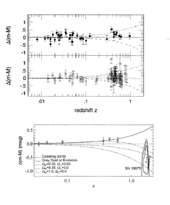
Figure 1: Hubble diagram of Type Ia Supernovas minus an empty ($\Omega_{0}$) Universe compared to cosmological models. All data in the upper panel have been normalized with the same $(\Delta m_{15})$ method (Leibundgut [50]). The filled squares are the data from HZT [48], and those of SCP [47] are shown as open squares. The parameters $(\Omega_{M},\Omega_{\Lambda})$ of the cosmological models are: (1,0) (long dashes), (0,1) (dashed line), (0.3,0.7) (dotted line). In the lower panel the points are redshift-binned data from both teams [52]. A typical curve for grey dust evolution is also shown. In spite of the large uncertainties of SN 1999ff at $z\simeq 1.7$, simple grey dust evolution seems to be excluded.

The main result of the analysis is presented in Fig.2. Keeping only $\Omega_{M}$ and $\Omega_{\Lambda}$ in Eq.(56) ( whence $\Omega_{K}=1-\Omega_{M}-\Omega_{\Lambda})$ in the fit to the data of 79 SNe Ia, and adopting the same luminosity width correction method ( $\Delta m_{15}$) for all of them, it shows the resulting confidence regions corresponding to 68.3%, 95.4%, and 99.7% probability in the $(\Omega_{M},\Omega_{\Lambda})$-plane. Taken at face value, this result excludes $\Omega_{\Lambda}=0$ for values of $\Omega_{M}$ which are consistent with other observations (e.g., of clusters of galaxies). This is certainly the case if a flat universe is assumed. The probability regions are inclined along $\Omega_{\Lambda}\approx 1.3\Omega_{M}+(0.3\pm 0.2)$. It will turn out that this information is largely complementary to the restrictions we shall obtain in Sect.6 from the CMB anisotropies.

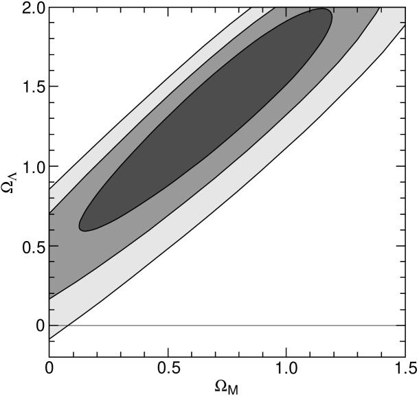
Figure 2: Likelihood regions in the $\Omega_{M}-\Omega_{\Lambda}$ plane for the data in Fig.1. Contours give the 68.3%, 95.4%, and 99.7% statistical confidence regions (adapted from [50]).

5.4 Systematic uncertainties

Possible systematic uncertainties due to astrophysical effects have been discussed extensively in the literature. The most serious ones are (i) dimming by intergalactic dust, and (ii) evolution of SNe Ia over cosmic time, due to changes in progenitor mass, metallicity, and C/O ratio. I discuss these concerns only briefly (see also [50], [51]).

Concerning extinction, detailed studies show that high-redshift SN Ia suffer little reddening; their B-V colors at maximum brightness are normal. However, it can a priori not be excluded that we see distant SNe through a grey dust with grain sizes large enough as to not imprint the reddening signature of typical interstellar extinction. One argument against this hypothesis is that this would also imply a larger dispersion than is observed. The discovery [52] of SN 1997ff with the very high redshift $z\approx 1.7$ led to the conclusion that its redshift and distance estimates are inconsistent with grey dust. Perhaps this statement is too strong, because a pair of galaxies in the foreground of SN 1997ff at $z=0.56$ may induce a magnification due to gravitational lensing of $\sim 0.3mag$ [53]. With more examples of this type the issue could be settled. Eq.(63) shows that at redshifts $z\geq(2\Omega_{\Lambda}/\Omega_{M})^{1/3}-1\simeq 1.2$ the Universe is decelerating, and this provides an almost unambiguous signature for $\Lambda$, or some effective equivalent.

The same SN has provided also some evidence against a simple luminosity evolution that could mimic an accelerating Universe. Other empirical constraints are obtained by comparing subsamples of low-redshift SN Ia believed to arise from old and young progenitors. It turns out that there is no difference within the measuring errors, after the correction based on the light-curve shape has been applied. Moreover, spectra of high-redshift SNe appear remarkably similar to those at low redshift. This is very reassuring. On the other hand, there seems to be a trend that more distant supernovas are bluer. It would, of course, be helpful if evolution could be predicted theoretically, but in view of what has been said earlier, this is not (yet) possible.

In conclusion, none of the investigated systematic errors appear to reconcile the data with $\Omega_{\Lambda}=0$ and $q_{0}\geq 0$. But further work is necessary before we can declare this as a really established fact.

To improve the observational situation a satellite mission called SNAP (“Supernovas Acceleration Probe”) has been proposed [54]. According to the plans this satellite would observe about 2000 SNe within a year and much more detailed studies could then be performed. For the time being some scepticism with regard to the results that have been obtained is not out of place.

Finally, I mention a more theoretical complication. In the analysis of the data the luminosity distance for an ideal Friedmann universe was always used. But the data were taken in the real inhomogeneous Universe. This may not be good enough, especially for high-redshift standard candles. The simplest way to take this into account is to introduce a filling parameter which, roughly speaking, represents matter that exists in galaxies but not in the intergalactic medium. For a constant filling parameter one can determine the luminosity distance by solving the Dyer-Roeder equation. But now one has an additional parameter in fitting the data. For a flat universe this was recently investigated in [55].

6 Microwave background anisotropies

By observing the cosmic microwave background (CMB) we can directly infer how the Universe looked at the time of recombination. Beside its spectrum, which is Planckian to an incredible degree [56], we also can study the temperature fluctuations over the “cosmic photosphere” at a redshift $z\approx 1100$. Through these we get access to crucial cosmological information (primordial density spectrum, cosmological parameters, etc). A major reason for why this is possible relies on the fortunate circumstance that the fluctuations are tiny ($\sim 10^{-5}$ ) at the time of recombination. This allows us to treat the deviations from homogeneity and isotropy for an extended period of time perturbatively, i.e., by linearizing the Einstein and matter equations about solutions of the idealized Friedmann-Lemaître models. Since the physics is effectively linear, we can accurately work out the evolution of the perturbations during the early phases of the Universe, given a set of cosmological parameters. Confronting this with observations, tells us a lot about the initial conditions, and thus about the physics of the very early Universe. Through this window to the earliest phases of cosmic evolution we can, for instance, test general ideas and specific models of inflation.

6.1 On the physics of CMB

Long before recombination (at temperatures $T>6000K$, say) photons, electrons and baryons were so strongly coupled that these components may be treated together as a single fluid. In addition to this there is also a dark matter component. For all practical purposes the two interact only gravitationally. The investigation of such a two-component fluid for small deviations from an idealized Friedmann behavior is a well-studied application of cosmological perturbation theory. (For the basic equations and a detailed analytical study, see [57] and [58].)

At a later stage, when decoupling is approached, this approximate treatment breaks down because the mean free path of the photons becomes longer (and finally ‘infinite’ after recombination). While the electrons and baryons can still be treated as a single fluid, the photons and their coupling to the electrons have to be described by the general relativistic Boltzmann equation. The latter is, of course, again linearized about the idealized Friedmann solution. Together with the linearized fluid equations (for baryons and cold dark matter, say), and the linearized Einstein equations one arrives at a complete system of equations for the various perturbation amplitudes of the metric and matter variables. There exist widely used codes [59], [60] that provide the CMB anisotropies – for given initial conditions – to a precision of about 1%.

A lot of qualitative and semi-quantitative insight into the relevant physics can be gained by looking at various approximations of the ‘exact’ dynamical system. Below I shall discuss some of the main points. (For well-written papers on this aspect I recommend [61], [62].)

For readers who want to skip this somewhat technical discussion and proceed directly to the observational results (Sect.6.2), the following qualitative remarks may be useful. A characteristic scale, which is reflected in the observed CMB anisotropies, is the sound horizon at last scattering, i.e., the distance over which a pressure wave can propagate until $\eta_{dec}$. This can be computed within the unperturbed model and subtends about one degree on the sky for typical cosmological parameters. For scales larger than this sound horizon the fluctuations have been laid down in the very early Universe. These have been detected by the COBE satellite. The (brightness) temperature perturbation $\Theta=\Delta T/T$ (defined precisely in Eq.(88) below) is dominated by the combination of the intrinsic temperature fluctuations and gravitational redshift or blueshift effects. For example, photons that have to climb out of potential wells for high-density regions are redshifted. In Sect.6.1.5 it is shown that these effects combine for adiabatic initial conditions to $\frac{1}{3}\Psi$, where $\Psi$ is the gravitational Bardeen potential (see Eq.(73)). The latter, in turn, is directly related to the density perturbations. For scale-free initial perturbations the corresponding angular power spectrum of the temperature fluctuations turns out to be nearly flat (Sachs-Wolfe plateau in Fig.3). The $C_{l}$ plotted in Fig.3 are defined in (109) as the expansion coefficients of the angular correlation function in terms of Legendre polynomials.

On the other hand, inside the sound horizon (for $\eta\leq\eta_{dec}$), acoustic, Doppler, gravitational redshift, and photon diffusion effects combine to the spectrum of small angle anisotropies shown in Fig.3. These result from gravitationally driven acoustic oscillations of the photon-baryon fluid, which are damped by photon diffusion (Sect.6.1.4).

6.1.1 Cosmological perturbation theory

Unavoidably, the detailed implementation of what has just been outlined is somewhat complicated, because we are dealing with quite a large number of dynamical variables. This is not the place to develop cosmological perturbation theory in any detail , but I have to introduce some of it.

Mode decomposition

Because we are dealing with slightly perturbed Friedmann spacetimes we may regard the various perturbation amplitudes as time dependent functions on a three-dimensional Riemannian space $(\Sigma,\gamma)$ of constant curvature $K$. Since such a space is highly symmetrical we are invited to perform two types of decompositions.

In a first step we split the perturbations into scalar, vector, and tensor contributions. This is based on the following decompositions of vector and symmetric tensor fields on $\Sigma$ : A vector field $\xi$ is a unique sum of a gradient and a vector field $\xi_{*}$ with vanishing divergence,

$$\xi=\xi_{*}+\nabla f,\;\;\;\nabla\cdot\xi_{*}=0.$$ (64)

(If $\Sigma$ is noncompact we have to impose some fall-off conditions.) The first piece $\xi_{*}$ is the ‘vector’ part, and $\nabla f$ is the ‘scalar’ part of $\xi$. This is a special case of the Hodge decomposition for differential forms. For a symmetric tensor field $S_{ij}$ we have correspondingly :

$$S_{ij}=S_{ij}^{(scalar)}+S_{ij}^{(vector)}+S_{ij}^{(tensor)},$$ (65)

with

$$S_{ij}^{(scalar)} = \gamma_{ij}S^{k}{}_{k}+(\nabla_{i}\nabla_{j}-\frac{1}{3}\gamma_{ij}\Delta)f,$$ (66)

$$S_{ij}^{(vector)} = \nabla_{i}\xi_{j}+\nabla_{j}\xi_{i},$$ (67)

with $\nabla_{k}\xi^{k}=0$, and where $S_{ij}^{(tensor)}$ is a symmetric tensor field with vanishing trace and zero divergence.

The main point is that these decompositions respect the covariant derivative $\nabla$ on $(\Sigma,\gamma)$. For example, if we apply the Laplacian on (64) we readily obtain

$$\Delta\xi=\Delta\xi_{*}+\nabla(\Delta f+2Kf),$$

and here the first term has vanishing divergence. For this reason the different components in the perturbation equations do not mix.

In a second step we can perform a harmonic decomposition, in expanding all amplitudes in terms of generalized spherical harmonics on $(\Sigma,\gamma)$. For $K=0$ this is just Fourier analysis. Again the various modes do not mix, and very importantly, the perturbation equations become for each mode ordinary differential equations. (From the Boltzmann equation we get an infinite hierarchy; see below.)

Gauge transformations, gauge invariant amplitudes

In general relativity the diffeomorphism group of spacetime is an invariance group. This means that the physics is not changed if we replace the metric $g$ and all the matter variables simultaneously by their diffeomorphically transformed objects. For small amplitude departures from some unperturbed situation, $g=g^{(0)}+\delta g$, etc., this implies that we have the gauge freedom

$$\delta g\longrightarrow\delta g+L_{\xi}g^{(0)},\;\;\;etc.,$$ (68)

where $L_{\xi}$ is the Lie derivative with respect to any vector field $\xi$. Sets of metric and matter perturbations which differ by Lie derivatives of their unperturbed values are physically equivalent. Such gauge transformations induce changes in the various perturbation amplitudes. It is clearly desirable to write all independent perturbation equations in a manifestly gauge invariant manner. Then one gets rid of uninteresting gauge modes, and misinterpretations of the formalism are avoided.

Let me show how this works for the metric. The most general scalar perturbation $\delta g$ of the Friedmann metric

$$g^{(0)}=dt^{2}-a^{2}(t)\gamma=a^{2}(t)\Bigl{[}d\eta^{2}-\gamma\Bigr{]}$$ (69)

can be parameterized as follows

$$\delta g=2a^{2}(\eta)\Bigl{[}Ad\eta^{2}+B_{,i}dx^{i}d\eta-(D\gamma_{ij}+E_{|ij})dx^{i}dx^{j}\Bigr{]}.$$ (70)

The functions $A(\eta,x^{i}),B,D,E$ are the scalar perturbation amplitudes; $E_{|ij}$ denotes the second covariant derivative $\nabla_{i}\nabla_{j}E$ on $(\Sigma,\gamma)$. It is easy to work out how $A,B,D,E$ change under a gauge transformation (68) for a vector field $\xi$ of ‘scalar’ type: $\xi=\xi^{0}\partial_{0}+\xi^{i}\partial_{i},$ with $\xi^{i}=\gamma^{ij}\xi_{|j}$. From the result one can see that the following Bardeen potentials [64]

$$\Psi = A-\frac{1}{a}\Bigl{[}a(B+E^{\prime})\Bigr{]}^{\prime},$$ (71)

$$\Phi = D-\mathcal{H}(B+E^{\prime})$$ (72)

are gauge invariant. Here, a prime denotes the derivative with respect to the conformal time $\eta$, and $\mathcal{H}=a^{\prime}/a$. The potentials $\Psi$ and $\Phi$ are the only independent gauge invariant metric perturbations of scalar type. One can always chose the gauge such that only the $A$ and $D$ terms in (70) are present. In this so-called longitudinal or conformal Newtonian gauge we have $\Psi=A,\Phi=D$, hence the metric becomes

$$g=a^{2}(\eta)\Bigl{[}(1+2\Psi)d\eta^{2}-(1+2\Phi)\gamma_{ij}dx^{i}dx^{j}\Bigr{]}.$$ (73)

Boltzmann hierarchy

Boltzmann’s description of kinetic theory in terms of a one particle distribution function finds a natural setting in general relativity. The metric induces a diffeomorphism between the tangent bundle $TM$ and the cotangent bundle $T^{*}M$ over the spacetime manifold $M$. With this the standard symplectic form on $T^{*}M$ can be pulled back to $TM$. In natural bundle coordinates the diffeomorphism is: $(x^{\mu},p^{\alpha})\mapsto(x^{\mu},p_{\alpha}=g_{\alpha\beta}p^{\beta})$ , hence the symplectic form on $TM$ is given by

$$\omega_{g}=dx^{\mu}\wedge d(g_{\mu\nu}p^{\nu}).$$ (74)

The geodesic spray is the Hamiltonian vector field $X_{g}$ on $(TM,\omega_{g})$ belonging to the “Hamiltonian function” $L=\frac{1}{2}g_{\mu\nu}p^{\mu}p^{\nu}$. Thus, in standard notation,

$$i(X_{g})\;\omega_{g}=dL.$$ (75)

In bundle coordinates

$$X_{g}=p^{\mu}\frac{\partial}{\partial x^{\mu}}-\Gamma^{\mu}{}_{\alpha\beta}p^{\alpha}p^{\beta}\frac{\partial}{\partial p^{\mu}}.$$ (76)

The integral curves of this vector field satisfy the canonical equations

$$\frac{dx^{\mu}}{d\lambda} = p^{\mu},$$ (77)

$$\frac{dp^{\mu}}{d\lambda} = -\Gamma^{\mu}{}_{\alpha\beta}p^{\alpha}p^{\beta}.$$ (78)

The geodesic flow is the flow of $X_{g}$. The Liouville volume form $\Omega_{g}$ is proportional to the fourfold wedge product of $\omega_{g}$, and has the bundle coordinate expression

$$\Omega_{g}=(-g)dx^{0123}\wedge dp^{0123},$$ (79)

where $dx^{0123}\equiv dx^{0}\wedge dx^{1}\wedge dx^{2}\wedge dx^{3}$, etc… The one-particle phase space for particles of mass $m$ is the submanifold $\Phi_{m}=\{v\in TM\mid g(v,v)=m^{2}\}$ of $TM$. This is invariant under the geodesic flow. The restriction of $X_{g}$ to $\Phi_{m}$ will also be denoted by $X_{g}$. $\Omega_{g}$ induces a volume form $\Omega_{m}$ on $\Phi_{m}$, which is remains invariant under $X_{g}$, thus $L_{X_{g}}\Omega_{m}=0$. A simple calculation shows that $\Omega_{m}=\eta\wedge\Pi_{m}$, where $\eta$ is the standard volume form of $(M,g)$, $\eta=\sqrt{-g}dx^{0123}$, and $\Pi_{m}=\sqrt{-g}dp^{123}/p_{0},p_{0}$ being determined by $g_{\mu\nu}p^{\mu}p^{\nu}=m^{2}$.
Let $f$ be a distribution function on $\Phi_{m}$. The particle number current density is

$$n^{\mu}(x)=\int_{P_{m}(x)}fp^{\mu}\Pi_{m},$$ (80)

where $P_{m}(x)$ is the fiber over $x$ in $\Phi_{m}$ (all momenta with $g(p,p)=m^{2})$. Similarly, the energy-momentum tensor is

$$T^{\mu\nu}=\int fp^{\mu}p^{\nu}\Pi_{m}.$$ (81)

One can show that

$$\nabla_{\mu}n^{\mu}=\int_{P_{m}}(L_{X_{g}}f)\Pi_{m},$$ (82)

and

$$\nabla_{\nu}T^{\mu\nu}=\int_{P_{m}}p^{\mu}(L_{X_{g}}f)\Pi_{m}.$$ (83)

The Boltzmann equation has the form

$$L_{X_{g}}f=C[f],$$ (84)

where $C[f]$ is the collision term. If this is (for instance) inserted into (83), we get an expression for the divergence of $T^{\mu\nu}$ in terms of a collision integral. For collisionless particles (neutrinos) this vanishes, of course.

Turning to perturbation theory, we set again $f=f^{(0)}+\delta f$, where $f^{(0)}$ is the unperturbed distribution function of the Friedmann model. For the perturbation $\delta f$ we choose as independent variables $\eta,x^{i},q,\gamma^{j}$, where $q$ is the magnitude and the $\gamma^{j}$ the directional cosines of the momentum vector relative to an orthonormal triad field $\hat{e}_{i}(i=1,2,3)$ of the unperturbed spatial metric $\gamma$ on $\Sigma$.

¿From now on we consider always the massless case (photons). By investigating the gauge transformation behavior of $\delta f$ [68] one can define a gauge invariant perturbation $\mathcal{F}$ which reduces in the longitudinal gauge to $\delta f$ (there are other choices possible [68]), and derive with some effort the following linearized Boltzmann equation for photons:

$$(\partial_{\eta}+\gamma^{i}\hat{e}_{i})\mathcal{F}-\hat{\Gamma}^{i}{}_{jk}\gamma^{j}\gamma^{k}\frac{\partial\mathcal{F}}{\partial\gamma^{i}}-q\Bigl{[}\Phi^{\prime}+\gamma^{i}\hat{e}_{i}\Psi\Bigr{]}\frac{\partial f^{(0)}}{\partial q}=$$ (85)

$$ax_{e}n_{e}\sigma_{T}\Bigl{[}<\mathcal{F}>-\mathcal{F}-q\frac{\partial f^{(0)}}{\partial q}\gamma^{i}\hat{e}_{i}V_{b}+\frac{3}{4}Q_{ij}\gamma^{i}\gamma^{j}\Bigr{]}.$$

On the left, the $\hat{\Gamma}^{i}{}_{jk}$ denote the Christoffel symbols of $(\Sigma,\gamma)$ relative to the triad $\hat{e}_{i}$. On the right, $x_{e}n_{e}$ is the unperturbed free electron density ($x_{e}=$ ionization fraction), $\sigma_{T}$ the Thomson cross section, and $V_{b}$ the gauge invariant scalar velocity perturbation of the baryons. Furthermore, we have introduced the spherical averages

$$<\mathcal{F}> = \frac{1}{4\pi}\int_{S^{2}}\mathcal{F}d\Omega_{\gamma},$$ (86)

$$Q_{ij} = \frac{1}{4\pi}\int_{S^{2}}[\gamma_{i}\gamma_{j}-\frac{1}{3}\delta_{ij}]\mathcal{F}d\Omega_{\gamma}.$$ (87)

In our applications to the CMB we work with the gauge invariant brightness temperature perturbation

$$\Theta(\eta,x^{i},\gamma^{j})=\int\mathcal{F}q^{3}dq\;\Big{/}\;\;4\int f^{(0)}q^{3}dq.$$ (88)

(The factor $4$ is chosen because of the Stephan-Boltzmann law, according to which $\delta\rho/\rho=4\delta T/T.$) It is simple to translate (85) to the following equation for $\Theta$

$$(\Theta+\Psi)^{\prime}+\gamma^{i}\hat{e}_{i}(\Theta+\Psi)-\hat{\Gamma}^{i}{}_{jk}\gamma^{j}\gamma^{k}\frac{\partial}{\partial\gamma^{i}}(\Theta+\Psi)=$$ (89)

$$(\Psi^{\prime}-\Phi^{\prime})+\dot{\tau}(\theta_{0}-\Theta+\gamma^{i}\hat{e}_{i}V_{b}+\frac{1}{16}\gamma^{i}\gamma^{j}\Pi_{ij}),$$

with $\dot{\tau}=x_{e}n_{e}\sigma_{T}a/a_{0},\;\theta_{0}=<\Theta>$ (spherical average),

$$\frac{1}{12}\Pi_{ij}=\frac{1}{4\pi}\int[\gamma_{i}\gamma_{j}-\frac{1}{3}\delta_{ij}]\Theta\;d\Omega_{\gamma}.$$ (90)

Let me from now on specialize to the spatially flat case $(K=0)$. In a mode decomposition (Fourier analysis of the $x^{i}$-dependence), and introducing the brightness moments $\theta_{l}(\eta)$ by

$$\Theta(\eta,k^{i},\gamma^{j})=\sum_{l=0}^{\infty}(-i)^{l}\theta_{l}(\eta,k)P_{l}(\mu),\;\;\;\mu=\mbox{\boldmath$\hat{k}\cdot\gamma$},$$ (91)

we obtain

$$\Theta^{\prime}+ik\mu(\Theta+\Psi)=-\Phi^{\prime}+\dot{\tau}[\theta_{0}-\Theta-i\mu V_{b}-\frac{1}{10}\theta_{2}P_{2}(\mu)].$$ (92)

It is now straightforward to derive from the last two equations the following hierarchy of ordinary differential equations for the brightness moments $\theta_{l}(\eta)$:

$$\theta_{0}^{\prime} = -\frac{1}{3}k\theta_{1}-\Phi^{\prime},$$ (93)

$$\theta_{1}^{\prime} = k\Bigl{(}\theta_{0}+\Psi-\frac{2}{5}\theta_{2}\Bigr{)}-\dot{\tau}(\theta_{1}-V_{b}),$$ (94)

$$\theta_{2}^{\prime} = k\Bigl{(}\frac{2}{3}\theta_{1}-\frac{3}{7}\theta_{3}\Bigr{)}-\dot{\tau}\frac{9}{10}\theta_{2},$$ (95)

$$\theta_{l}^{\prime} = k\Bigl{(}\frac{l}{2l-1}\theta_{l-1}-\frac{l+1}{2l+3}\theta_{l+1}\Bigr{)},\;\;\;l>2.$$ (96)

The complete system of perturbation equations

Without further ado I collect below the complete system of perturbation equations. For this some additional notation has to be fixed.

Unperturbed background quantities: $\rho_{\alpha},p_{\alpha}$ denote the densities and pressures for the species $\alpha=b$ (baryon and electrons), $\gamma$ (photons), $c$ (cold dark matter); the total density is the sum $\rho=\sum_{\alpha}\rho_{\alpha}$, and the same holds for the total pressure $p$. We also use $w_{\alpha}=p_{\alpha}/\rho_{\alpha},w=p/\rho$. The sound speed of the baryon-electron fluid is denoted by $c_{b}$, and $R$ is the ratio $3\rho_{b}/4\rho_{\gamma}$.

Here is the list of gauge invariant scalar perturbation amplitudes (for further explanations see [65]):

• $\delta_{\alpha},\delta$ : density perturbations ($\delta\rho_{\alpha}/\rho_{\alpha},\delta\rho/\rho\;$ in the longitudinal gauge); clearly: $\rho\;\delta=\sum\rho_{\alpha}\delta_{\alpha}$.

• $V_{\alpha},V$ : velocity perturbations; $\rho(1+w)V=\sum_{\alpha}\rho_{\alpha}(1+w_{\alpha})V_{\alpha}.$

• $\theta_{l},N_{l}$ : brightness moments for photons and neutrinos.

• $\Pi_{\alpha},\Pi$ : anisotropic pressures; $\Pi=\Pi_{\gamma}+\Pi_{\nu}$. For the lowest moments the following relations hold:

  $$\delta_{\gamma}=4\theta_{0},\;\;V_{\gamma}=\theta_{1},\;\;\Pi_{\gamma}=\frac{12}{5}\theta_{2},$$ (97)

  and similarly for the neutrinos.

• $\Psi,\Phi$: Bardeen potentials for the metric perturbation.

As independent amplitudes we can choose: $\delta_{b},\delta_{c},V_{b},V_{c},\Phi,\Psi,\theta_{l},N_{l}$. The basic evolution equations consist of three groups.

• Fluid equations:

  $$\delta_{c}^{\prime} = -kV_{c}-3\Phi^{\prime},$$ (98)

  $$V_{c}^{\prime} = -aHV_{c}+k\Psi;$$ (99)

  $$\delta_{b}^{\prime} = -kV_{b}-3\Phi^{\prime},$$ (100)

  $$V_{b}^{\prime} = -aHV_{b}+kc^{2}_{b}\delta_{b}+k\Psi+\dot{\tau}(\theta_{1}-V_{b})/R.$$ (101)

• Boltzmann hierarchies for photons (Eqs. (93)-(96)) and the collisionless neutrinos.

• Einstein equations : We only need the following algebraic ones for each mode:

  $$k^{2}\Phi = 4\pi Ga^{2}\rho\Bigl{[}\delta+3\frac{aH}{k}(1+w)V\Bigr{]},$$ (102)

  $$k^{2}(\Phi+\Psi) = -8\pi Ga^{2}p\;\Pi.$$ (103)

In arriving at these equations some approximations have been made which are harmless , except for one: We have ignored polarization effects in Thomson scattering. For quantitative calculations these have to be included. Moreover, polarization effects are highly interesting, as I shall explain later.

6.1.2 Angular correlations of temperature fluctuations

The system of evolution equations has to be supplemented by initial conditions. We can not hope to be able to predict these, but at best their statistical properties (as, for instance, in inflationary models). Theoretically, we should thus regard the brightness temperature perturbation $\Theta(\eta,x^{i},\gamma^{j})$ as a random field. Of special interest is its angular correlation function at the present time $\eta_{0}$. Observers measure only one realization of this, which brings unavoidable cosmic variances.

For further elaboration we insert (91) into the Fourier expansion of $\Theta$, obtaining

$$\Theta(\eta,\mbox{\boldmath$x$},\mbox{\boldmath$\gamma$})=(2\pi)^{-\frac{3}{2}}\int d^{3}k\sum_{l}\theta_{l}(\eta,k)G_{l}(\mbox{\boldmath$x$},\mbox{\boldmath$\gamma$};\mbox{\boldmath$k$}),$$ (104)

where

$$G_{l}(\mbox{\boldmath$x$},\mbox{\boldmath$\gamma$};\mbox{\boldmath$k$})=(-i)^{l}P_{l}(\mbox{\boldmath$\hat{k}\cdot\gamma$})\exp(i\mbox{\boldmath$k\cdot x$}).$$ (105)

Hence we have

$$\Theta(\eta,\mbox{\boldmath$x$},\mbox{\boldmath$\gamma$})=\sum_{lm}a_{lm}^{*}Y_{lm}(\mbox{\boldmath$\gamma$}),$$ (106)

with

$$a_{lm}=(2\pi)^{-\frac{3}{2}}\int d^{3}k\;\theta_{l}(\eta,k)\;i^{l}\frac{4\pi}{2l+1}Y_{lm}(\mbox{\boldmath$\hat{k}$})\exp(-i\mbox{\boldmath$k\cdot x$}).$$ (107)

We expect on the basis of rotation invariance that the two-point correlation of the random variables $a_{lm}$ has the form

$$<a_{lm}a_{l^{\prime}m^{\prime}}^{*}>=C_{l}\delta_{ll^{\prime}}\delta_{mm^{\prime}}.$$ (108)

¿From (106) and (108) we see that the angular correlation function of $\Theta$ in x-space is

$$<\Theta(\mbox{\boldmath$\gamma$})\Theta(\mbox{\boldmath$\gamma^{\prime}$})>=\sum_{l}\frac{2l+1}{4\pi}C_{l}P_{l}(\mbox{\boldmath$\gamma\cdot\gamma^{\prime}$}).$$ (109)

If different modes in k-space are uncorrelated, we obtain from (107)

$$\frac{2l+1}{4\pi}C_{l}=\frac{1}{2\pi^{2}}\int_{0}^{\infty}\frac{dk}{k}\frac{k^{3}|\theta_{l}(k)|^{2}}{2l+1}.$$ (110)

Cosmic variance

The $C_{l}$ are the expectation values of the stochastic variable

$$Z=\frac{1}{2l+1}\sum_{m}a_{lm}a_{lm}^{*}.$$

If the $a_{lm}$ are Gaussian random variables, as in simple inflationary models, then the variance of $Z$, and thus of $C_{l}$, is easily found to be given by

$$\sigma(C_{l})=\sqrt{\frac{2}{2l+1}}.$$ (111)

This is a serious limitation for low multipoles that cannot be overcome. For large $l$ the measured $C_{l}$ should be accurately described by (110), taken at the present time.

6.1.3 Brightness moments in sudden decoupling

The linearized Boltzmann equation in the form (92) as an inhomogeneous linear differential for the $\eta$-dependence has the ‘solution’

$$(\Theta+\Psi)(\eta_{0},\mu;k)=$$ (112)

$$\int_{0}^{\eta_{0}}d\eta\Bigl{[}\dot{\tau}(\theta_{0}+\Psi-i\mu V_{b}-\frac{1}{10}\theta_{2}P_{2})+\Psi^{\prime}-\Phi^{\prime}\Bigr{]}e^{-\tau(\eta,\eta_{0})}e^{ik\mu(\eta-\eta_{0})},$$

where

$$\tau(\eta,\eta_{0})=\int_{\eta}^{\eta_{0}}\dot{\tau}d\eta$$ (113)

is the optical depth. The combination $\dot{\tau}e^{-\tau}$ is the (conformal) time visibility function. It has a simple interpretation: Let $p(\eta,\eta_{0})$ be the probability that a photon did not scatter between $\eta$ and today ($\eta_{0}$). Clearly, $p(\eta-d\eta,\eta_{0})=p(\eta,\eta_{0})(1-\dot{\tau}d\eta)$. Thus $p(\eta,\eta_{0})=e^{-\tau(\eta,\eta_{0})}$, and the visibility function times $d\eta$ is the probability that a photon last scattered between $\eta$ and $\eta+d\eta$. The visibility function is therefore strongly peaked near decoupling. This is very useful, both for analytical and numerical purposes.

In order to obtain an integral representation for the multipole moments $\theta_{l}$, we insert in (112) for the $\mu$-dependent factors standard expansions in terms of Legendre polynomials. For $l\geq 2$ we find the following useful formula:

$$\frac{\theta_{l}(\eta_{0})}{2l+1}=\int_{0}^{\eta_{0}}d\eta e^{-\tau(\eta)}\Bigl{[}(\dot{\tau}\theta_{0}+\dot{\tau}\Psi+\Psi^{\prime}-\Phi^{\prime})j_{l}(k(\eta_{0}-\eta))+\dot{\tau}V_{b}j_{l}^{\prime}+\dot{\tau}\frac{1}{20}\theta_{2}(3j_{l}^{\prime\prime}+j_{l})\Bigr{]}.$$ (114)

In a reasonably good approximation we can replace the visibility function by a $\delta$-function, and obtain (with $\Delta\eta\equiv\eta_{0}-\eta_{dec},V_{b}(\eta_{dec})\simeq\theta_{1}(\eta_{dec})$:

$$\frac{\theta_{l}(\eta_{0},k)}{2l+1}\simeq[\theta_{0}+\Psi](\eta_{dec},k)j_{l}(k\Delta\eta)+\theta_{1}(\eta_{dec},k)j_{l}^{\prime}(k\Delta\eta)+ISW+Quad.$$ (115)

Here, the quadrupole contribution (last term) is not important. ISW denotes the integrated Sachs-Wolfe effect:

$$ISW=\int_{\eta_{dec}}^{\eta_{0}}d\eta(\Psi^{\prime}-\Phi^{\prime})j_{l}(k\Delta\eta),$$ (116)

which only depends on the time variations of the Bardeen potentials between recombination and the present time.

The interpretation of the first two terms in (115) is quite obvious: The first describes the fluctuations of the effective temperature $\theta_{0}+\Psi$ on the cosmic photosphere, as we would see them for free streaming between there and us, – if the gravitational potentials would not change in time. ($\Psi$ includes blue- and redshift effects.) The dipole term has to be interpreted, of course, as a Doppler effect due to the velocity of the baryon-photon fluid.

In this approximate treatment we only have to know the effective temperature $\theta_{0}+\Psi$ and the velocity moment $\theta_{1}$ at decoupling. The main point is that eq.(115) provides a good understanding of the physics of the CMB anisotropies. Note that the individual terms are all gauge invariant. In gauge dependent methods interpretations would be ambiguous.

6.1.4 Acoustic oscillations

In this subsection we derive from the Boltzmann hierarchy (93)-(96) an approximate equation for the effective temperature fluctuation $\Delta T\equiv\theta_{0}+\Psi$, which will teach us a lot.

As long as the mean free path of photons is much shorter than the wavelength of the fluctuation, the optical depth through a wavelength $\sim\dot{\tau}/k$ is large. Thus the evolution equations may be expanded in $k/\dot{\tau}$.

In lowest order we obtain $\theta_{1}=V_{b},\;\theta_{l}=0$ for $l\geq 2$, thus $\delta_{b}^{\prime}=3\theta_{0}^{\prime}$. Going to the first order, we can replace on the right of the following form of eq.(94),

$$\theta_{1}-V_{b}=\frac{R}{\dot{\tau}}[V_{b}^{\prime}+\frac{a^{\prime}}{a}V_{b}-k\Psi],$$ (117)

$V_{b}$ by $\theta_{1}$:

$$\theta_{1}-V_{b}=\frac{R}{\dot{\tau}}[\theta_{1}^{\prime}+\frac{a^{\prime}}{a}\theta_{1}-k\Psi].$$ (118)

We insert this in (94), and set in first order $\theta_{2}=0$. Using also $a^{\prime}/a=R^{\prime}/R$ we get

$$\theta_{1}^{\prime}=\frac{1}{1+R}k\theta_{0}+k\Psi-\frac{R^{\prime}}{1+R}\theta_{1}.$$ (119)

Together with (93) we find the driven oscillator equation

$$\theta_{0}^{\prime\prime}+\frac{R^{\prime}}{1+R}\frac{a^{\prime}}{a}\theta_{0}^{\prime}+c_{s}^{2}k^{2}\theta_{0}=F(\eta),$$ (120)

where

$$c_{s}^{2}=\frac{1}{3(1+R)},\;\;F(\eta)=-\frac{k^{2}}{3}\Psi-\frac{R}{1+R}\frac{a^{\prime}}{a}\Phi^{\prime}-\Phi^{\prime\prime}.$$ (121)

The damping term is due to expansion. In second order one finds an additional damping term proportional to $\theta_{0}^{\prime}$:

$$\frac{1}{3}\frac{k^{2}}{\dot{\tau}}\Bigl{[}(\frac{R}{1+R})^{2}+\frac{8}{9}\frac{1}{1+R}\Bigr{]}\theta_{0}^{\prime}.$$ (122)

This describes the damping due to photon diffusion (Silk damping).

We discuss here only the first order equation, which we rewrite in the more suggestive form ($m_{eff}\equiv 1+R$)

$$(m_{eff}\theta_{0}^{\prime})^{\prime}+\frac{k^{2}}{3}(\theta_{0}+m_{eff}\Psi)=-(m_{eff}\Phi^{\prime})^{\prime}.$$ (123)

This equation may be interpreted as follows: The change in momentum of the photon-baryon fluid is determined by a competition between pressure restoring and gravitational driving forces.

Let us, in a first step, ignore the time dependence of $m_{eff}$ (i.e., of the baryon-photon ratio $R$), then we get a forced harmonic oscillator equation

$$m_{eff}\theta_{0}^{\prime\prime}+\frac{k^{2}}{3}\theta_{0}=-\frac{k^{2}}{3}m_{eff}\Psi-(m_{eff}\Phi^{\prime})^{\prime}.$$ (124)

The effective mass $m_{eff}=1+R$ accounts for the inertia of baryons. Baryons also contribute gravitational mass to the system, as is evident from the right hand side of the last equation. Their contribution to the pressure restoring force is, however, negligible.

We now ignore in (124) also the time dependence of the gravitational potentials $\Phi,\Psi$. With (121) this then reduces to

$$\theta_{0}^{\prime\prime}+k^{2}c_{s}^{2}\theta_{0}=-\frac{1}{3}k^{2}\Psi.$$ (125)

This simple harmonic oscillator under constant acceleration provided by gravitational infall can immediately be solved:

$$\theta_{0}(\eta)=[\theta_{0}(0)+(1+R)\Psi]\cos(kr_{s})+\frac{1}{kc_{s}}\dot{\theta}_{0}(0)\sin(kr_{s})-(1+R)\Psi,$$ (126)

where $r_{s}(\eta)$ is the comoving sound horizon $\int c_{s}d\eta$. One can show that for adiabatic initial conditions there is only a cosine term. In this case we obtain for $\Delta T$:

$$\Delta T(\eta,k)=[\Delta T(0,k)+R\Psi]\cos(kr_{s}(\eta))-R\Psi.$$ (127)

Discussion

In the radiation dominated phase ($R=0$) this reduces to $\Delta T(\eta)\propto\cos kr_{s}(\eta)$, which shows that the oscillation of $\theta_{0}$ is displaced by gravity. The zero point corresponds to the state at which gravity and pressure are balanced. The displacement $-\Psi>0$ yields hotter photons in the potential well since gravitational infall not only increases the number density of the photons, but also their energy through gravitational blue shift. However, well after last scattering the photons also suffer a redshift when climbing out of the potential well, which precisely cancels the blue shift. Thus the effective temperature perturbation we see in the CMB anisotropies is – as remarked in connection with eq. (115) – indeed $\Delta T=\theta_{0}+\Psi$. It is clear from (127) that a characteristic wave-number is $k=\pi/r_{s}(\eta_{dec})\simeq\pi/c_{s}\eta_{dec}$. A spectrum of $k$-modes will produce a sequence of peaks with wave numbers

$$k_{m}=m\pi/r_{s}(\eta_{dec}),\;\;m=1,2,...$$ (128)

Odd peaks correspond to the compression phase (temperature crests), whereas even peaks correspond to the rarefaction phase (temperature troughs) inside the potential wells. Note also that the characteristic length scale $r_{s}(\eta_{dec})$, which is reflected in the peak structure, is determined by the underlying unperturbed Friedmann model. This comoving sound horizon at decoupling depends on cosmological parameters, but not on $\Omega_{\Lambda}$. Its role will further be discussed in Sect.6.2. Inclusion of baryons not only changes the sound speed, but gravitational infal leads to greater compression of the fluid in a potential well, and thus to a further displacement of the oscillation zero point (last term in(127). This is not compensated by the redshift after last scattering, since the latter is not affected by the baryon content. As a result all peaks from compression are enhanced over those from rarefaction. Hence, the relative heights of the first and second peak is a sensitive measure of the baryon content. We shall see that the inferred baryon abundance from the present observations is in complete agreement with the results from big bang nucleosynthesis.

What is the influence of the slow evolution of the effective mass $m_{eff}=1+R$? Well, from the adiabatic theorem we know that for a slowly varying $m_{eff}$ the ratio energy/frequency is an adiabatic invariant. If $A$ denotes the amplitude of the oscillation, the energy is $\frac{1}{2}m_{eff}\omega^{2}A^{2}$. According to (121) the frequency $\omega=kc_{s}$ is proportional to $m_{eff}^{-1/2}$. Hence $A\propto\omega^{-1/2}\propto m_{eff}^{1/4}\propto(1+R)^{-1/4}$.

6.1.5 Angular power spectrum for large scales

The angular power spectrum is defined as $l(l+1)C_{l}$ versus $l$. For large scales, i.e., small $l$, observed with COBE, the first term in eq.(115) dominates. Let us have a closer look at this so-called Sachs-Wolfe contribution.

For large scales (small $k$) we can neglect in the first equation (93) of the Boltzmann hierarchy the term proportional to $k$: $\theta_{0}^{\prime}\approx-\Phi^{\prime}\approx\Psi^{\prime}$, neglecting also $\Pi$ (i.e., $\theta_{2}$) on large scales. Thus

$$\theta_{0}(\eta)\approx\theta_{0}(0)+\Psi(\eta)-\Psi(0).$$ (129)

To proceed, we need a relation between $\theta_{0}(0)$ and $\Psi(0)$. This can be obtained by looking at superhorizon scales in the tight coupling limit. (Alternatively, one can investigate the Boltzmann hierarchy in the radiation dominated era.) For adiabatic initial perturbations one easily finds $\theta_{0}(0)=-\frac{1}{2}\Psi(0)$, while for the isocurvature case one gets $\theta_{0}(0)=\Psi(0)=0$. Using this in (129), and also that $\Psi(\eta)=\frac{9}{10}\Psi(0)$ in the matter dominated era, we find for the effective temperature fluctuations at decoupling

$$(\theta_{0}+\Psi)(\eta_{dec})=\frac{1}{3}\Psi(\eta_{dec})$$ (130)

for the adiabatic case. For initial isocurvature fluctuations the result is six times larger. Eq.(130) is due to Sachs and Wolfe. It allows us to express the angular CMB power spectrum on large scales in terms of the power spectrum of density fluctuations at decoupling. If the latter has evolved from a scale free primordial spectrum, it turns out that $l(l+1)C_{l}$ is constant for small $l^{\prime}s$. It should be emphasized that on these large scales the power spectrum remains close to the primordial one.

Having discussed the main qualitative aspects, we show in Fig.3 a typical theoretical CMB power spectrum for scale free adiabatic initial conditions.

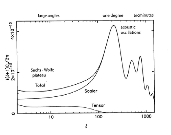
Figure 3: Theoretical angular power spectrum for adiabatic initial perturbations and typical cosmological parameters. The scalar and tensor contributions to the anisotropies are also shown.

6.2 Observational results

CMB anisotropies had been looked for ever since Penzias and Wilson’s discovery of the CMB, but had eluded all detection until the Cosmic Background Explorer (COBE) satellite discovered them on large angular scales in 1992 [69]. It is not at all astonishing that it took so long in view of the fact that the temperature perturbations are only one part in $10^{-5}$ (after subtraction of the obvious dipole anisotropy). There are great experimental difficulties to isolate the cosmologically interesting signal from foreground contamination. The most important of these are: (i) galactic dust emission; (ii) galactic thermal and synchrotron emission; (iii) discrete sources; (iv) atmospheric emission, in particular at frequencies higher than $\sim$10 GHz.

After 1992 a large number of ground and balloon-borne experiments were set up to measure the anisotropies on smaller scales. Until quite recently the measuring errors were large and the data had a considerable scatter, but since early 2001 the situation looks much better. Thanks to the experiments BOOMERanG [70], MAXIMA [71] and DASI [72] we now have clear evidence for multiple peaks in the angular power spectrum at positions and relative heights that were expected on the basis of the simplest inflationary models and big bang nucleosynthesis.

Wang et al. [73] have compressed all available data into a single band-averaged set of estimates of the CMB power spectrum. Their result, together with the $\pm 1\sigma$ errors, is reproduced in Fig.4. These data provide tight constraints for the cosmological parameters. However, the CMB anisotropies alone do not fix them all because there are unavoidable degeneracies, especially when tensor modes (gravity waves) are included. This degeneracy is illustrated in Fig.9 of Ref.[70] by three best fits that are obtained by fixing $\Omega_{b}h_{0}^{2}$ in a reasonable range.

Figure 4: Band-averaged CMB power spectrum, together with the $\pm 1\sigma$ errors (Fig.2 of Ref. [70]).

Such degeneracies can only be lifted if other cosmological information is used. Beside the supernova results, discussed in Sect.5, use has been made, for instance, of the available information for the galaxy power spectrum. In [74] the CMB data have been combined with the power spectrum of the $2dF$ (2-degree-Field) Galaxy Redshift Survey (2dFGRS). The authors summarize their results of the combined likelihood analysis in Table 1 of their paper. Here, I quote only part of it. The Table below shows the $\pm 2\sigma$ parameter ranges for some of the cosmological parameters, for two types of fits. In the first only the CMB data are used (but tensor modes are included), while in the second these data are combined with the 2dFGRS power spectrum (assuming adiabatic, Gaussian initial conditions described by power laws).

Table 1
Parameter	CMB alone	CMB and 2dFGRS
$\Omega_{b}h_{0}^{2}$	0.016-0.045	0.018-0.034
$\Omega_{c}h_{0}^{2}$	0.03-0.18	0.07-0.13
$\Omega_{K}$	-0.68-0.06	-0.05-0.04
$\Omega_{\Lambda}$	$<$0.88	0.65-0.85

Note that $\Omega_{K}$ is not strongly constraint by CMB alone. However, if $h_{0}$ is assumed a priori to be within a reasonable range, then $\Omega_{K}$ has to be close to zero (flat universe). It is very satisfying that the combination of the CMB and 2dFGRS data constrain $\Omega_{\Lambda}$ in the range $0.65\leq\Omega_{\Lambda}\leq 0.85$. This is independent of – but consistent with – the supernova results.

Another beautiful result has to be stressed. For the baryon parameter $\Omega_{b}h_{0}^{2}$ there is now full agreement between the CMB results and the BBN prediction. Earlier speculations in connection with possible contradictions now have evaporated. The significance of this consistency cannot be overemphasized.

All this looks very impressive. It is, however, not forbidden to still worry about possible complications located in the initial conditions, for which we have no established theory. For example, an isocurvature admixture cannot be excluded and the primordial power spectrum may have unexpected features.

Temperature measurements will not allow us to isolate the contribution of gravitational waves. This can only be achieved with future sensitive polarization experiments. Polarization information will provide crucial clues about the physics of the very early Universe. It can, for instance, be used to discriminate between models of inflation. With the Planck satellite, currently scheduled for launch in February 2007, it will be possible to detect gravitational waves even if they contribute only 10 percent to the anisotropy signal.

7 Quintessence

For the time being, we have to live with the mystery of the incredible smallness of a gravitationally effective vacuum energy density. For most physicists it is too much to believe that the vacuum energy constitutes the missing two thirds of the average energy density of the present Universe. This would really be bizarre. The goal of quintessence models is to avoid such an extreme fine-tuning. In many ways people thereby repeat what has been done in inflationary cosmology. The main motivation there was, as is well-known, to avoid excessive fine tunings of standard big bang cosmology (horizon and flatness problems).

In concrete models the exotic missing energy with negative pressure is again described by a scalar field, whose potential is chosen such that the energy density of the homogeneous scalar field adjusts itself to be comparable to the matter density today for quite generic initial conditions, and is dominated by the potential energy. This ensures that the pressure becomes sufficiently negative. It is not simple to implement this general idea such that the model is phenomenologically viable. For instance, the success of BBN should not be spoiled. CMB and large scale structure impose other constraints. One also would like to understand why cosmological acceleration started at about $z\sim 1$, and not much earlier or in the far future. There have been attempts to connect this with some characteristic events in the post-recombination Universe. On a fundamental level, the origin of a quintessence field that must be extremely weakly coupled to ordinary matter, remains in the dark.

There is already an extended literature on the subject. Refs. [75] - [81] give a small selection of important early papers and some recent reviews. I conclude by emphasizing again that on the basis of the vacuum energy problem we would expect a huge additive constant for the quintessence potential that would destroy the hole picture. Thus, assuming for instance that the potential approaches zero as the scalar field goes to infinity, has (so far) no basis. Fortunately, future more precise observations will allow us to decide whether the presently dominating exotic energy density satisfies $p/\rho=-1$ or whether this ratio is somewhere between $-1$ and $-1/3$. Recent studies (see [82], [83], and references therein) which make use of existing CMB data, SN Ia observations and other information do not yet support quintessence with $w_{Q}>-1$.

However, even if convincing evidence for this should be established, we will not be able to predict the distant future of the Universe. Eventually, the quintessence energy density may perhaps become  negative. This illustrates that we may never be able to predict the asymptotic behavior of the most grandiose of all dynamical systems. Other conclusions are left to the reader.

References

- [1] S.Weinberg, Rev.Mod.Phys. 61, 1 (1989).
- [2] A.Einstein, Sitzungsber. Preuss. Akad. Wiss. phys.-math. Klasse VI, 142 (1917). See also: Ref.[2], Vol. 6, p.540, Doc. 43.
- [3] A.Einstein, The Collected Papers of Albert Einstein.-Princeton University Press; Vol. 8, Part A, p.386, Doc.294.
- [4] A.Pais, ‘Subtle is the Lord…’: The Science and the Life of Albert Einstein. Oxford University Press (1982). See especially Sect.15e.
- [5] W.de Sitter, Proc. Acad. Sci., 19, 1217 (1917); and 20, 229 (1917).
- [6] A.S.Eddington, The Mathematical Theory of Relativity.Chelsea Publishing Company (1924). Third (unaltered) Edition (1975). See especially Sect.70.
- [7] J.D.North, The Measure of the Universe: A History of Modern Cosmology. Oxford: Clarendon Press (1965). Reprinted: Dover (1990).
- [8] H.Weyl, Raum, Zeit, Materie. Fifth Edition. Springer-Verlag, Berlin (1923). See especially Appendix III.
- [9] A.Friedmann, Z.Phys. 10, 377 (1922); 21, 326 (1924).
- [10] G.Lemaître, Ann. Soc. Sci. Brux. A 47, 49 (1927).
- [11] A.Einstein, S.B. preuss. Akad. Wiss. (1931), 235.
- [12] A.Einstein, Appendix to the 2nd edn. of The Meaning of Relativity, (1945); reprinted in all later editions.
- [13] W.Pauli, Theory of Relativity. Pergamon Press (1958); Supplementary Note 19.
- [14] O.Heckmann, Theorien der Kosmologie, berichtigter Nachdruck, Springer-Verlag (1968).
- [15] N.Straumann, General Relativity and Relativistic Astrophysics, Springer-Verlag (1984).
- [16] V.Petrosian, E.E.Salpeter, and P. Szekeres, Astrophys. J. 147, 1222 (1967).
- [17] W.Pauli, Pauli Lectures on Physics; Ed. C.P.Enz. MIT Press (1973); Vol.4, especially Sect.20.
- [18] C.P.Enz, and A.Thellung, Helv. Phys. Acta 33, 839 (1960).
- [19] Y.B.Zel’dovich, JETP letters 6, 316 (1967); Soviet Physics Uspekhi 11, 381 (1968).
- [20] W.Pauli, Die allgemeinen Prinzipien der Wellenmechanik. Handbuch der Physik, Vol. XXIV (1933). New edition by N.Straumann, Springer-Verlag (1990); see Appendix III, p. 202.
- [21] H.B.G.Casimir, Kon.Ned.Akad.Wetensch. B51, 793 (1948).
- [22] S.K.Lamoreaux, quant-ph/9907076.
- [23] P.Jordan and W.Pauli, Z. Phys.47, 151 (1928).
- [24] M.Bordag, U.Mohideen, and V.M.Mostepanenko New Developments in the Casimir Effect, quant-ph/0106045.
- [25] W.Heisenberg and H.Euler, Z. Phys. 38, 714 (1936).
- [26] V.S.Weisskopf, Kongelige Danske Videnskabernes Selskab, Mathematisk-fysiske Meddelelser XIV, No.6 (1936).
- [27] L.D.Landau and E.M.Lifshitz, Quantum Electrodynamics, Vol.4, second edition, Pergamon Press (1982); Sect.129.
- [28] W.Dittrich and M.Reuter, Lecture Notes in Physics, Vol.220 (1985).
- [29] E.Zavattini et al.; S.Askenazy et al., in Quantum Electrodynamics and Physics of the Vacuum, edited by G.Cantatore, American Institute of Physics, 2001 (p.77, 115).
- [30] M.Kardar and R.Golestanian, Rev. Mod. Phys.71,1233, (1999).
- [31] G.A.Tammann, A.Sandage, and A.Saha, astro-ph/0010422.
- [32] C.G.Callan, S.Coleman, and R.Jackiw, Ann.Phys.59, 42 (1970).
- [33] T.Schäfer and E.V. Shuryak, Rev. Mod. Phys. 70,,323 (1998).
- [34] R.D.Peccei and H.Quinn, Phys. Rev. Lett, 38, 1440 (1977); Phys. Rev. D16, 1791 (1977).
- [35] E.Witten, hep-ph/0002297.
- [36] S.M.Caroll, Living Reviews in Relativity, astro-ph/0004075.
- [37] N.Straumann, in Dark Matter in Astro- and Particle Physics, Edited by H.V.Klapdor-Kleingrothaus, Springer (2001), p.110.
- [38] S.E.Rugh and H.Zinkernagel, hep-th/0012253.
- [39] W.Baade, Astrophys. J.88,285 (1938).
- [40] G.A.Tammann. InAstronomical Uses of the Space Telescope, eds. F.Macchetto, F.Pacini and M.Tarenghi, p.329. Garching: ESO.
- [41] S.Colgate, Astrophys. J.232,404 (1979).
- [42] SCP-Homepage: http://www-supernova.LBL.gov
- [43] HZT-Homepage: http://cfa-www.harvard.edu/cfa/oir/Research/supernova/HighZ.html
- [44] Cosmic Explosions, eds. S.Holt and W.Zhang, AIP, in press.
- [45] W.Hillebrandt and J.C.Niemeyer, Ann. Rev. Astron. Astrophys. 38,191-230 (2000).
- [46] B.Leibundgut, Astron. Astrophys.10, 179 (2000).
- [47] S.Perlmutter, et al., Astrophys. J.517, 565 (1999).
- [48] B.Schmidt, et al., Astrophys. J.507, 46 (1998).
- [49] A.G.Riess, et al., Astron. J.116, 1009 (1998).
- [50] B.Leibundgut, Ann. Rev. Astron. Astrophys.39, 67 (2001).
- [51] A.Fillipenko and A.Riess, astro-ph/9905049; astro-ph/0008057.
- [52] A.G.Riess, et al., astro-ph/0104455.
- [53] G.F.Lewis and R.A.Ibata, astro-ph/0104254.
- [54] Snap-Homepage: http://snap.lbl.gov
- [55] R.Kantowski and R.C.Thomas, Astrophys. J.561, 491 (2001); astro-ph/0011176.
- [56] D.J.Fixsen, et al., Astrophys. J.473, 576 (1996).
- [57] H.Kodama and M.Sasaki, Internat. J. Mod. Phys.A1, 265 (1986).
- [58] H.Kodama and M.Sasaki, Internat. J. Mod. Phys.A2, 491 (1987).
- [59] U.Seljak, and M. Zaldarriaga, Astrophys.. J.469, 437 (1996). (See also http://www.sns.ias.edu/matiasz/CMBFAST/cmbfast.html)
- [60] A.Lewis, A.Challinor and A.Lasenby, Astrophys. J.538, 473 (2000).
- [61] W.Hu and N.Sugiyama, Astrophys. J.444, 489 (1995).
- [62] W.Hu and N.Sugiyama, Phys. Rev.D51, 2599 (1995).
- [63] A.R.Liddle and D.H.Lyth, Cosmological Inflation and Large-Scale Structure. Cambridge University Press (2000).
- [64] J.Bardeen, Phys. Rev.D22, 1882 (1980).
- [65] H.Kodama and M.Sasaki, Progr. Theor. Phys. Suppl.78, 1 (1984).
- [66] R.Durrer, Fund. of Cosmic Physics15, 209 (1994).
- [67] N.Straumann, Cosmological Perturbation Theory. Unpublished lecture notes, to be made available.
- [68] R.Durrer and N.Straumann, Helvetica Phys. Acta,61, 1027 (1988).
- [69] G.F.Smoot, et al., Astrophys. J. 396, L1 (1992).
- [70] C.B.Netterfield, et al., astro-ph/0104460; S.Masi, et al., astro-ph/0201137.
- [71] A.T.Lee, et al., astro-ph/0104459.
- [72] N.W.Halverson, et al., astro-ph/0104489.
- [73] X.Wang M.Tegmark and M.Zaldarriaga, astro-ph/0105091.
- [74] G.Efstathiou, et al., astro-ph/0109152.
- [75] C.Wetterich, Nucl. Phys. B302, 668 (1988).
- [76] B.Ratra and P.J.E.Peebles, Astrophys. J. Lett. 325, L17 (1988); Phys. Rev. D37, 3406 (1988).
- [77] R.R.Caldwell, R.Dave and P.J.Steinhardt, Phys. Rev. Lett.80,1582 (1998).
- [78] P.J.Steinhardt, L.Wang and I.Zlatev, Phys. Rev. Lett.82, 896 (1999); Phys. Rev. D59, 123504 (1999).
- [79] C.Armendariz-Picon, V.Mukhanov and P.J.Steinhardt, astro-ph/0004134 and astro-ph/0006373.
- [80] P.Binétruy, hep-ph/0005037.
- [81] C.Wetterich, University of Heidelberg preprint, (2001).
- [82] R.Bean, S.H. Hansen, and A.Melchiorri, astro-ph/0201127.
- [83] C.Baccigalupi et al., astro-ph/0109097.