The evolution of the Mira variable R Hydrae

Abstract

The Mira variable R Hydrae is well known for its declining period, which Wood & Zarro (1981) attributed to a possible recent thermal pulse. Here we investigate the long-term period evolution, covering 340 years, going back to its discovery in AD 1662. The data includes photometric monitoring by amateur and other astronomers over the last century, and recorded dates of maximum for earlier times. Wavelets are used to determine both the period and semi-amplitude. We show that the period decreased linearly between 1770 and 1950; since 1950 the period has stabilized at 385 days. The semi-amplitude is shown to closely follow the period evolution. Analysis of the oldest data shows that before 1770 the period was about 495 days. We find no evidence for an increasing period during this time as found by Wood & Zarro. We discuss the mass-loss history of R Hya: the IRAS data shows that the mass loss dropped dramatically around AD 1750. The evolution of the mass loss as function of period agrees with the mass-loss formalism from Vassiliadis & Wood; it is much larger than predicted by the Blöcker law. An outer detached IRAS shell suggests that R Hya has experienced mass-loss interruptions before. The period evolution can be explained by two models: a thermal pulse occuring around AD 1600, or an non-linear instability leading to an internal relaxation of the stellar structure. The elapsed time between the mass-loss decline giving rise to the outer detached shell, and the recent event, of approximately 5000 yr suggests that only one of these events could be due to a thermal pulse. Further monitoring of R Hya is recommended, as both models make strong predictions for the future period evolution. We argue that R Hya-type events could provide part of the explanation for the rings seen around some AGB and post-AGB stars. Changes in Mira properties were already known on a cycle-to-cycle basis, and on the thermal-pulse time scale of $\sim 10^{4}\,\rm yr$. R Hya shows that significant evolution can also occur on intermediate time scales of order $10^{2}$–$10^{3}\,\rm yr$.

1 Introduction

R Hya is an unusual Mira variable. Miras are long-period variables found near the tip of the Asymptotic Giant Branch (AGB). They show mono-periodic light curves with large visual amplitudes of more than 2.5 mag. The periods are typically 200–500 days; the amplitude and shape of the light curve can vary over time but the periods tend to be stable. Optical data covering a century or more confirm the remarkable stability of the Mira pulsations (e.g. Sterken et al. 1999). But in sharp contrast to this rule, the period of R Hya has been declining steadily for over a century.

Although period jitter of a few per cent is common among Miras (Lombard & Koen, 1993), possibly related to small changes in the shape of the light curves, there are only a few examples of significant period evolution. Other types of changes appear to be more common, but stars which exhibit them are automatically classified as semiregular (SR): the Mira classification requires pulsation stability. The SR class is a mixture of hidden Miras and non-Mira stars. Examples of the former include R Dor (located on the Mira $PL$ relation) which shows sudden switches between a period of 330 days and one of 180 days (Bedding et al., 1998), indicative of mode switching. V Boo has shown an almost complete disappearance of its Mira pulsation over a century, albeit without any change in its period (Szatmary et al., 1996). But only R Aql is known to show a continuous period decline similar to that of R Hya.

Early AGB stars contain a helium-burning shell. But during the last 10% of the AGB, when the helium becomes exhausted, the shell switches to hydrogen burning, punctuated by regular helium flashes: the thermal pulses (Vassiliadis & Wood, 1993; Boothroyd & Sackmann, 1988). Wood & Zarro (1981) argue that a recent thermal pulse could explain the period change of R Hya, if the star is presently in the luminosity decline following the peak of the pulse. This interpretation has generally been followed in other papers discussing period evolution, e.g. on R Cen and T UMi (Hawkins, Mattei & Foster, 2001; Whitelock, 1999; Mattei & Foster, 2000; Gal & Szatmary, 1995). In support of their interpretation, Wood & Zarro (1981) find that the earliest observations of R Hya indicate an increasing period, which they explain with the luminosity increase immediately after the onset of the thermal pulse.

In this paper we analyse data of R Hya going back to its discovery in AD 1662. The light curve is subjected to wavelet analysis, which shows how the period and amplitude (the latter available only since 1900) have evolved over time. We find that the decline in period is accompanied by a decline in amplitude. We also find that the period is no longer decreasing, having stabilised at 385 days in about 1950. The period was about 495 days before 1770; and we do not confirm the reported early period increase. R Hya appears to have evolved to its present stable period over approximately 200 yr.

The paper is organised as follows: In Section 2 we describe the data and the analysis methods. Section 3 contains a detailed discussion of the period evolution. In Section 4 we discuss the characteristics of the star. Section 5 discusses the pulsation evolution in terms of proposed AGB relations. Section 6.1 discusses the mass-loss history and Section 6.2 describes the two models which can explain R Hya-type behaviour. and show that the circumstellar rings observed. Finally, in Section 6.3 er discuss a possible relation to the rings observed around AGB and post-AGB stars. The conclusions are summarized in Section 7.

2 Observations

2.1 The data

Many bright long-period variable stars have been monitored by amateur astronomers. The observations can be found in public archives. These archives are valuable resources, and complement high-precision photometry datasets (e.g., Hipparcos, MACHO) that only cover a few years.

The magnitudes are determined by eye, using reference fields that contain stars with a range of known magnitudes: a magnitude for the target star is established by comparison with this standard sequence. The accuracy is typically 0.1 mag. For red stars, systematic differences may exist between observers. When using such data, sufficient observations from each individual source should be available to test for individual accuracy and systematic offsets.

For R Hya (HR 5080; HIP 65835), we used data from the American Association of Variable Star Observers (AAVSO), the Variable Star Observers League of Japan (VSOLJ), the Association Francaise des Observateurs d’Etoiles Variables (AFOEV) and the British Astronomical Association, Variable Star Section (BAAVSS). Only data from individual observers contributing 30 or more observations were used and we did not attempt to correct for offsets between observers. Fig. 1 shows the combined data, binned to 10-day averages.

Figure 1: The light curve, using data taken from the AAVSO (11347 points), AFOEV (1489 points), BAAVS (4369 points) and VSOLJ (1509 points), binned to 10-day averages

Before about AD 1890, the compilations of Cannon & Pickering (1909) and Müller & Hartwig (1918) give derived dates of maxima (and, more rarely, minima), but these do not include individual measurements. These data can give a reasonable estimate for the period if sufficient successive maxima are available.

2.2 Light curve analysis

Mira light curves are often analyzed using the so-called O–C technique (where O stands for the observed date of maximum and C for the calculated date). The O–C technique must be used with care when searching for secular period changes because it can be affected by period jitter: a small jitter can lead to large phase differences over long time scales (Lombard & Koen, 1993). In this paper we prefer the use of wavelet transforms.

Wavelets are useful when the pulsation properties change over time, and have been used to study long-period variables (e.g., Szatmary et al. 1996; Bedding et al. 1998; Kiss et al. 1999). We use the weighted wavelet Z-transform (WWZ: Foster 1996) developed at AAVSO specifically for uneven sampled data.

We experimented with different values for the parameter $c$, which defines the tradeoff between time resolution and frequency resolution (Foster, 1996), and settled on $c=0.005$ as a good compromise. More details of the application of the WWZ transform to long-period variables are given by Bedding et al. (1998).

3 The period evolution of R Hya

3.1 AD 1850–2001

Fairly complete coverage is available since 1850, as dates of maxima for 1850–1900 (Cannon & Pickering, 1909; Müller & Hartwig, 1918), and as individual magnitude estimates since 1900. To allow wavelet analysis, the pre-1900 dates of maxima and minima were arbitrarily assigned magnitudes of 5.0 and 10.0, respectively. In many cases only dates of maxima were available, and results from the wavelet analysis could only be obtained by inserting the missing minima. This was only done when it was clear that consecutive maxima had been measured, in which case the date of the minimum was taken as being midway between the maxima.

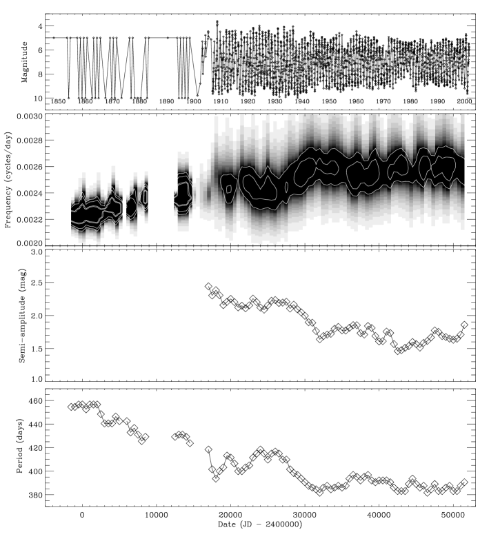
Figure 2: The wavelet analysis for R Hya, 1850–2000. Shown are: the light curve, the frequency, the semi-amplitude of the main frequency component and its period.

Fig. 2 shows the wavelet plot for R Hya. The lightcurve is shown in the top panel, and the arbitrary magnitudes assigned to pre-1900 dates of maxima and minima are obvious. The second panel shows the WWZ transform, with the grey scale indicating the significance of each frequency as a function of time (see Bedding et al. 1998). Only a small range of frequencies is shown – there was no evidence for significant power outside this range. The third and fourth panels show, for each time bin, the semi-amplitude (in magnitudes) and period (in days) corresponding to the peak of the WWZ in the second panel. Note that semi-amplitudes are not available from these data prior to 1900.

The period evolution in R Hya is clearly visible, with an overall decline between 1850 and 1950, from 455 days to 385 days. There is significant period jitter in addition to the decline. Before 1900, some of the jitter may be due to the uncertainty in the dates of maxima. (Different determinations of the same maximum can typically differ by a few days to a week, but occasionally much more.)

As made clear in Fig. 2, the period of R Hya is no longer decreasing (Greaves, 2000). With hindsight, we can say that the period stabilized at $\sim$385 days in about 1950, since which time the period jitter has been limited to the range 380–395 days. This jitter is within the normal range of Mira variables (Koen & Lombard, 1995). The period stabilization was preceded by a short phase of rapid decline, almost 10% within two decades.

Another result is the behaviour in the semi-amplitude. There was a decrease from 2.2 mag to 1.7 mag between 1910 and 1950, closely mimicking the period evolution. The rapid period decline around 1940 is especially well matched by the amplitude, as is the constancy of the amplitude since 1950. Fig. 3 shows the close relation between the semi-amplitude and period. We have reported similar behaviour in the Mira variables R Aql, BH Cru and S Ori (Bedding et al., 2000) and we speculated that, at least in some cases, the amplitude changes might cause the period changes via non-linear effects. For R Hya, the semi-amplitude reached a minimum around 1975, and has slowly increased again since.

Figure 3: Relation between period and semi-amplitude, from post-1910 observations. The trend visible in the upper right part of the plot, of decreasing amplitude with decreasing period, relates to the 1910–1950 data. The group of points in the lower part which show scatter contain the post-1950 data.

3.2 AD 1784–1850

Table 1 lists all recorded dates of maxima before 1850, based on information given by Müller & Hartwig (1918), Argelander (1869) and Cannon & Pickering (1909). The data are too patchy for wavelet analysis because the majority of maxima were not observed. Instead, we determined the period from observations of maxima that were consecutive or separated by only a few cycles. Since the period at 1850 is clearly established as $\sim$450 days (see above), we start from that date and work backwards.

Table 1: Pre-1850 observations of R Hya. Data taken from Müller & Hartwig (1918) and Cannon & Pickering (1909)

Year, month, date of maximum	observer
1662 04 18	Heveliusa
1670/2b 04 15	Montanaria
1704 03 20	Maraldic
1705 09 01:	Maraldid
1708 05 20	Maraldi
1709 11 01:	Maraldi
1712 05 15:	Maraldi
1784 01 26	Pigott
1785 05 25	Pigotte
1805 05 05	Piazzi
1809 04 04	Piazzi
1818 03 31:	Olbers f
1823 04 18	Olbers
1827 01 30	Schwerd
1843 05 30	Argelander
1848 04 23	Argelanderg

^a These are dates of observations rather than dates of maxima. However, given the magnitude range these observations could only have been made within 1–2 months of maximum.
^b There are two possible dates for this observations (see text).
^c Chandler (Astronomische Nachrichten 2463) derived the five maxima based on Maraldi’s data. Dates in the table are as given by Argelander: Maraldi gives 1704 March 14 and 1708 May 22. ^d The uncertain dates of maximum are as given by Müller & Hartwig (1918). The uncertainties are due to the fact that the maximum was not covered, or in one case (1712) was difficult to observe because of the Full Moon. We estimate the uncertainties as 1–2 months.
^e Pigott mentions simultaneous observations by Goodricke which have not been published.
^f He also reports observations between 14 March and 4 May 1817, post-maximum, and between 13 Feb and 15 May 1822, also with an earlier maximum.
^g The date of this maximum is given by Schmidt (independent observation) as 3 (or 5) May.

Argelander’s extensive observations gave maxima in 1843 and 1848, consistent with a period close to 450 days and implying that three intervening maxima were missed. Olbers (who discovered the period evolution) observed maxima in 1818 and 1823, which give a period of about 460 days (assuming three missing maxima), which also matches the maximum observed by Schwerd in 1827 (assuming two missing maxima). Maxima observed by Piazzi in 1805 and 1809 imply a period of 477 days, assuming two missing maxima. Finally, the maxima observed by Pigott in 1784 and 1785 were 485 days apart and were presumably consecutive.

Note that many of the unobserved maxima mentioned above would have occurred at times of the year when R Hya was not readily observable from Europe, as shown in Fig. 5. Together, these results suggest that the period of R Hya was decreasing during 1784–1850 at roughly the same rate as the post-1850 decline, as shown in Fig. 6.

3.3 AD 1662–1712

Unfortunately, there is an 80-year gap in observations of R Hya prior to those by Pigott in 1784. The sparse observing record reflects the poor observability: at the star’s southern declination ($-23\deg$), evening observations from Europe are feasible only in March–May (an early morning observation is required in winter), and even from Paris the star never reaches an airmass less than 3. But the large gap in the data also coincides with the depths of the Little Ice Age, with indications for increased cloud cover over Northern Europe (Neuberger, 1970).

We are therefore left with the observations of R Hya made in the first decades after its discovery, which we now describe in (forward) chronological order. The details are taken from papers by Argelander (1869), Müller & Hartwig (1918) and Hoffleit (1997). The first of these, in particular, contains a wealth of historical information on several Mira variables.

The first recorded observation of R Hya was by Johannes Hevelke (1611–1689; latinized Hevelius), who included it in his second catalogue (Hevelius, 1679) but did not note any variability. The observations were made from Gdansk, Poland, on the evenings of Tuesday 18 and Wednesday 19 April 1662.

The magnitude found by Hevelius is not certain. In his catalogue (Hevelius, 1690b), he gives it as a 6th mag star, but according to Maraldi (see below) Hevelius observed it at 5th magnitude (Argelander, 1869). Argelander states that he does not know how Maraldi obtained this value. However, Maraldi is likely to be correct: R Hya is indicated on Hevelius’ Uranographia (Hevelius, 1690a) (published shortly after this death) as of similar brightness to $\psi$ Hydra ($m_{V}=4.97$). The included stars are consistent with a brightness limit in this southerly region at $m_{V}=5$. The chart of Hevelius (1690a) is reproduced in Fig. 4. In the region below R Hya, a group of stars with magnitudes of 5.5 and fainter are lacking. Cannon & Pickering (1909) gave the discovery observation as the date of maximum, but Argelander (1869) argued that the real maximum occurred up to 2 months earlier or later. But if the star was a magnitude brighter than assumed by Argelander, it could have been closer to maximum.

Given this brightness limit, the variable U Hydrae should also be within the range of the catalogue. This carbon star varies between visual magnitudes of 4.7 and 5.7. It indeed appears to be present in the chart. There may be other, even older Chinese records of this variable (Hoffleit, 1997), although its semi-regular variability was not discovered until 1871. We have not investigated U Hya further, but note that the stars shown in this region are also consistent with a limit of little fainter than 5.0.

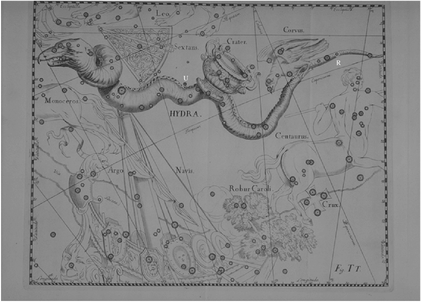
Figure 4: Hevelius (1690a) chart of the region, showing both R Hya and U Hya. R Hya is the faint star in the tail of Hydra, to the right of the tail of the crow: it is just to the right of $\gamma$ Hydrae and $\psi$ Hydrae. U Hydrae is located between Sextans and Crater, just above the body of Hydra.

Geminiano Montanari, independently and before Hevelius’ catalogue was published, observed R Hya while working at the Paris Observatory. While comparing Bayer’s Uranometry with the sky, he noticed an unmarked 4^th magnitude star along the line connecting $\psi$ and $\gamma$ Hya. Montanari did not publish the discovery and it is not known whether he noticed the variability. (Montanari had discovered the variability of $\beta$ Per a few years earlier.) He entered the star with its magnitude on the map of Bayer. The date of his observation was 15 April in either 1670 or 1672 (see below).

The variability of R Hya was first established by Giacomo Filippo Maraldi (the nephew of Cassini). In 1702 he tried to re-identify R Hya based on Montanari’s chart, but failed. But in March 1704 he observed the star and followed its appearances and disappearances until 1712 and identified maxima in 1704 and 1708. According to Müller & Hartwig (1918), Maraldi suspected a period of two years but, as they point out, this contradicts his own observations. They quote Pigott as deriving a period of 494 days in 1786 from his own and Maraldi’s observations. As we can see in Fig. 5, this period fits the five maxima of 1704–1712 very well. The period also agrees with Maraldi’s failure to detect the star in 1702, when it would have been near minimum.

The accuracy of the dates of maximum should not be overstated. The high airmass worsens the effects of the colours of the comparison stars. Argelander (1869) classifies the maxima according to accuracy, but for even the best determinations (1784 & 1785, 1823, 1848) he estimates the uncertainty as 6–7 days.

The evidence seems convincing that the period of R Hya during the time of Maraldi was about 495 days. As can be seen in Fig. 6, this indicates that the rate of period decrease was much less in the 18th century than in the 19th.

We now turn to the two pre-1700 observations, by Hevelius (in 1662) and Montanari (in either 1670 or 1672). The uncertainty in the year of Montanari’s observation is unfortunate. The observation was published by Maraldi, along with his own observations, in the Memoires de Paris (pour l’an 1706 and 1709), where the date was given twice as April 1672 and twice as 1670. However, in his own calculations Maraldi consistently used 1670. On the other hand, Montanari himself did not mention the star in a short paper of an academic speech from 1671 or 1672, describing several novae, which could favour the later date. Argelander (1869) and Müller & Hartwig (1918) preferred 1670, while Cannon & Pickering (1909) gave 1672 as the more likely.

Figure 5: The dates of observations are shown with a sine curve to indicate the proposed variability of R Hya. The plotted sine curve has a constant period of 496 days until 1770, declines at 0.4 days per year until 1800 after which the decline is 0.78 days per year. (This is not a unique fit, due to the paucity of data.) The solid curves indicate the parts of the light curve where observations before midnight would have been possible from Europe: March–June with $m<7$. The dashed line extends this to include early morning observations.

Assuming that the observation by Hevelius was made close to maximum, any period close to that from Maraldi’s data predicts a minimum in or around April 1672. On the other hand, accepting 1670 as the correct date and using a period of 496 days, we find an excellent fit with the observation by Hevelius and also with those of Maraldi (see Fig. 5). On their own, the two observations on 1662 and 1670/2 are consistent with an almost unconstrained range of periods, and they can be made to fit any changing period. But the fact that Maraldi’s confirmed period also fits these older observations leads to the plausible hypothesis that the period at the time of discovery was constant, at about 496 days. We do not find support for the statement by Wood & Zarro (1981) that “four very old (1662-1708) and valuable dates of maximum … show that the period was increasing.”

With this assumption of constant period, all observed maxima from 1662 to 1712 can be fitted to within 3 weeks (with the exception of the poorly determined maximum in Nov. 1709, which is predicted 2 months earlier). Maxima would have occurred in February 1662 and in March 1670, in good agreement with actual measurements. The lack of repeat observations by Montanari is also explained: the figure shows that the star would have been difficult to find for 2–3 years after his observation.

3.4 The period evolution

Figure 6: The period evolution of R Hya between 1662 and 2001. The first point is uncertain; the period is well determined from 1704 onwards. Extrapolation of the linear decline suggests the decline began around 1770. The dashed line is the fit proposed by Chandler (1896).

In summary, the period was approximately 495 days around AD 1700, declining to 480 days by AD 1800, 450 days by AD 1850, 420 days in AD 1900 and 380 days in AD 1950. The decline was almost linear, at 0.58 days/year: extrapolation suggests that the decline may have started around 1770, but it is also possible that the decline was initially slower and began earlier. Unfortunately, the decline probably began during the long gap in observations. The phases of constant period after and (possibly) before the decline suggest the possibility that the star has evolved from one (quasi) stable period to another.

Fig. 5 shows how the observed dates of maxima fit with the period evolution. It is difficult to fit all observations with a purely linear period decline with a sudden onset. The fit used in the figure assumes a constant period until 1770, declining by 0.4 days per year between 1770 and 1810, with the decline increasing to 0.6 days per year after 1810. All dates of maxima before 1850 can be fitted well with this evolution. However, the constraints are relatively poor and equally good fits are feasible without assuming a gradual start to the period decline. Instead the result can be taken as evidence for some period jitter. The post-maximum observations of Olbers in 1817 and 1822 are indicated as maxima at 01 Feb of those years. The figure shows that in both cases, the window of observability indeed fell post-maximum.

The full period evolution is shown in Fig. 6. The dashed line is the fit proposed by Chandler (1896) in the third catalogue of variable stars. The sinusoidal component is not confirmed but the slope of his fit gives a good approximation until the period decline ended around 1950.

A linear decline implies a constant rate of change in fraction per cycle, $\delta=1.6\times 10^{-3}$. The time scale of the decline, defined as $\tau=P/\delta$, where $P$ is the initial (longest) period, is $\tau=880\,\rm yr$. This is an average time scale: the period evolution also showed significant jitter, with a fastest time scale (around 1940) of $\tau\approx 200\,\rm yr$.

Amplitude data, available since about 1890, show that the decline in period was accompanied by a decline in semi-amplitude, from 2.2 to 1.7 mag since 1905, or 5 mmag/cycle. The time scale for the amplitude decline, extrapolating back to 1770, is about 800 yr, the same as for the period decline. The relation between period and amplitude is roughly linear (Fig. 3). The visual amplitude of an oxygen-rich Mira depends on the temperature variation during the pulsation, leading to the formation of molecules (TiO, VO) during minimum which strongly absorb at optical wavelengths (Reid & Goldston, 2002). A relation between amplitude and period could therefore be strongly non-linear, but this is not seen in R Hya.

4 Stellar parameters

The main uncertainty in the mass and luminosity of R Hya derives from its uncertain distance. Unfortunately, the Hipparcos parallax is a non-detection: $1.6\pm 2.4$ mas. Whitelock, Marang & Feast (2000) found a distance of 140 pc, derived by placing R Hya on the Mira period–luminosity ($P$–$L$) relation. Eggen (1985, 1966) reported a proper-motion companion which gave a distance modulus of 6.1 (165 pc). Jura & Kleinmann (1992) favoured a distance of 110pc, based on a $P$–$L$ relation. Only the value of Eggen is consistent with Hipparcos at the 2-$\sigma$ level: these two are also the only direct measurements.

Using $d=165$ pc, the luminosity is $L=1.16\times 10^{4}\,\rm L_{\odot}$. The mean of the Eggen and Hipparcos distances, 400 pc, would already yield a luminosity above the classical AGB limit ($M_{\rm bol}=-7.2$: this limit can be exceeded in the case of hot bottom burning, but only for very large core masses: Bloecker & Schoenberner 1991). For this reason we will use Eggen’s distance in the discussion to follow.

Eggen (1985) argued that R Hya is located within the Hyades supergroup, with an age of $5$–$10\times 10^{8}\,\rm yr$. This would imply a progenitor mass for R Hya around $2\,\rm M_{\odot}$. The presence of technetium (⁹⁹Tc) in R Hya (Little et al., 1987) shows that the star is in the thermal pulsing phase of the AGB (e.g., Lebzelter & Hron 1999): this element is dredged-up during the thermal pulses but has a half life of $\sim 10^{5}\,\rm yr$, several times the interpulse time scale. Its abundance slowly increases during the TP-AGB. Tc is found in 15% of semiregulars but 75% of long-period Miras.

Infrared photometry was reported by Whitelock et al. (2000): phase-averaged magnitudes are $(J,H,K,L)_{0}=-1.07,-2.05,-2.45,-2.88)$ and the bolometric magnitude is $m_{\rm bol}=0.64$. The infrared colours indicate an effective temperature of $T_{\rm eff}=2830\,\rm K$ (Feast, 1996). The $\rm V-K\approx 9.5$ is consistent with this temperature (Bessell et al., 1998). Haniff et al. (1995) obtain a lower $T_{\rm eff}=2680\pm 70\,\rm K$ by fitting to the flux distribution between 1.04 and 3.45 microns. They also derive $T_{\rm eff}$ from an angular diameter measurement: they found $2570\,\rm K$ or $2760\,\rm K$, assuming fundamental pulsation mode or first overtone, respectively.

The luminosity, with the temperature derived by Feast (1996), yields a radius of $R\approx 450\,\rm R_{\odot}$. For our adopted distance, this predicts an angular diameter of 26 mas. The angular diameter has been measured at 902 nm as $34.1\pm 3.4\,\rm mas$ (Haniff et al., 1995), assuming an uniform disk, yielding a large radius of $R=590\,\rm R_{\odot}$. A correction for limb darkening and molecular opacities brings the value down to about $500\,\rm R_{\odot}$ for first overtone models; for the fundamental mode the effect is much less. Recently, Tuthill (priv. comm.) measured a near-infrared diameter of 24 mas, in much better agreement with the prediction above. Part of the difference between the two observations may be due to photospheric extensions which can be significant at 902 nm: the $K$-band is likely to be less affected by this (Feast, 1996). In addition, the earlier observation took place close to minimum (Tuthill, priv. comm), which in Miras occurs when the star is largest.

Whitelock et al. (2000) and Feast (1996) assumed that R Hya is presently located on the Mira $P$–$L$ relation. However, this requires a distance (140 pc), outside the 2-$\sigma$ confidence limit of Hipparcos. Given its period history, a location on the narrow $P$–$L$ relation may not be expected. The distance assumed in this paper would put R Hya slightly above or to the left of the relation, perhaps between the Mira and SR branches (Bedding & Zijlstra, 1998). The Hipparcos distance places the star significantly above the relation, a location in common with O-rich LMC Miras with $P>420\,\rm days$ (Feast et al., 1989; Zijlstra et al., 1996).

5 The pulsation

The gradual change in the period of R Hya implies that its pulsation mode has remained constant; its evolution is therefore related to a change in the stellar parameters.

The pulsation mode of R Hya is an open question, as it is for all Mira variables (Wood, 1990; Whitelock & Feast, 2000; Ya’Ari & Tuchman, 1999). Neither is it proven that R Hya exhibits the same pulsation mode as other Miras. The radius derived above is consistent with either the fundamental mode or with first overtone (e.g., Whitelock & Feast 2000: R Hya falls in between the two modes in their Fig. 1).

The pulsation equation, which relates the period $P$ (in days) to the radius $R$ and mass $M$ (in solar units) is given by:

$$\log P=1.5\log R-0.5\log M+\log Q,$$ (1)

for first overtone pulsators, where the pulsation constant $Q\approx 0.04$ (Fox & Wood, 1982), or

$$\log P=1.949\log R-0.9\log M-2.07$$ (2)

for fundamental mode pulsators (Wood, 1990). These equations yield masses for R Hya of $0.74\,\rm M_{\odot}$ and $3.0\,\rm M_{\odot}$, respectively. The large mass required for the fundamental mode provides an argument for the first overtone, or alternatively for questioning whether the measured angular diameter is identical to the pulsational diameter.

The two equations both imply that the period evolution was accompanied by a change in radius: the radius would have decreased by 14–18%, depending on pulsation mode. The pre-1770 radius would have been about $520\,\rm R_{\odot}$.

There are no direct observations to show how $T_{\rm eff}$ and $L$ changed during the period evolution. Wood & Zarro (1981) fitted a luminosity decline of 20%, based on the assumption that R Hya underwent a thermal pulse. Ya’Ari & Tuchman (1996) presented a different model for period evolution (see below) which does not require a change in luminosity. The lack of information on the luminosity evolution does not allow us to test these two models.

The $P$–$L$ relation derived from LMC Miras is given by:

$$M_{\rm bol}=-3.00\log P+\alpha$$ (3)

(Feast, 1996). This predicts a luminosity decrease of 25% for the period decline of R Hya. However, this should be taken as an upper limit, as R Hya is unlikely to have evolved along this relation: the $P$–$L$ relation is not an evolutionary sequence but rather a sequence of stars with different progenitor masses and metallicities. The evolutionary tracks of Vassiliadis & Wood (1993) cross the $P$–$L$ relation at almost constant luminosity, while the Whitelock evolutionary track found in globular clusters (Whitelock, 1986) is also shallower. But short-term evolution, such as that shown by R Hya, may not follow these sequences either.

Combining the relation between colour and period of Whitelock et al. (2000),

$$\left(J-K\right)_{0}=-(0.39\pm 0.15)+(0.71\pm 0.06)\log P,$$ (4)

with the $T_{\rm eff}$–colour relation from Feast (1996),

$$\log T_{\rm eff}=-0.59(J-K)_{0}+4.194,$$ (5)

yields an increase of $T_{\rm eff}$ for R Hya of 10%, i.e., from 2570 to the present 2830 K. Combining this with the radius change from the pulsation equation gives the counterintuitive result that the luminosity of R Hya has increased by 5% rather than decreased. Given the slope of the $P$–$L$ relation, this suggests that the slope of the temperature calibration used here is too steep. The temperature calibration averages Mira and non-Mira M-type stars. Using only Mira variables gives a more shallow relation:

$$\log T{\rm eff}=-0.474(J-K)_{0}+4.059,$$ (6)

which gives a 3% decrease in luminosity. These relations suggest a negligible change in luminosity. The assumption that R Hya remained on the AGB colour relations (at constant $L$) may be more realistic than that of R Hya following $P$–$L$ relations, which predict decreasing $L$.

Bessell et al. (1998) give relations between the $V-K$ colour index and $T_{\rm eff}$ for giants. The above temperature change implies a decrease in $V-K$ of about 0.7 mag. If R Hya evolved along the $K$-band $P$–$L$ relation,

$$M_{K}=-3.47\log P+\beta,$$ (7)

its $K$-band magnitude would have become fainter by 0.4 mag. In this case the $V$-band magnitude should have brightened by 0.3 mag since 1770. For the shallower Whitelock track (e.g., Bedding & Zijlstra 1998), the change at $K$ would be less and the brightening at $V$ closer to 0.7 mag.

The average visual magnitude has not changed significantly since 1910, as indicated by the light curve. However, this only covers a fraction of the period decline. The earliest measurement of Montanari indicated the star to be of magnitude 4. R Hya has not reached this magnitude during maximum since 1940, but this can be accounted for by the decline in amplitude and does not imply a change in average magnitude. It is unlikely that R Hya was ever much brighter than 4th mag, because of its absence from the oldest star catalogues. In contrast, compare the possible presence of $o$ Ceti in Hipparchus’ catalogue (Costantino, 2002; Manitius,, 1894) (the person, not the satellite) (but its absence from the version in the Almagest (Ptolemaeus, 137)), and possibly $\chi$ Cygni in Chinese and/or Korean records as a nova on 14 November 1404 (Hoffleit, 1997). But such observations do not allow us to test the relatively small changes in $V$ predicted above, which in any case predicts that R Hya would have been fainter rather than brighter.

The final assumption we could make is that R Hya was and remained on the AGB colour sequence. The AGB equation from Wood (1990), for first overtone pulsation (Feast, 1996), is given by

$$M_{\rm bol}=15.7\log T_{\rm eff}+1.884\log z-2.65\log M-59.1-15.7\Delta$$ (8)

where the last term represents deviations from the AGB. The relation for fundamental mode is slightly different. Combining with the pulsation equation, we find

$$M_{\rm bol}\propto-2.036\log P;\qquad\log T_{\rm eff}\propto-0.13\log P$$ (9)

(Feast, 1996). This would yield an increase in $T_{\rm eff}$ of 3% and a decrease in $L$ of 20%. Such changes would be well within the observational constraints. This parametrized AGB may not be valid within the Mira instability strip. Also, if the star is undergoing a thermal pulse as suggested by Wood & Zarro (1981), it could be evolving on a blue loop rather than on the AGB sequence. This would give a higher temperature and higher (or constant) luminosity.

It is clear that the various relations are not mutually consistent. A luminosity decrease in R Hya is possible but is not proven. Only the radius change, obtained from the period, appears well constrained.

6 Discussion

6.1 Mass loss evolution: winds of change

There are strong observational relations between stellar parameters and mass loss on the TP-AGB. Blöcker (1995) proposed a variation of the Reimers mass-loss equation:

$$\dot{M}_{\rm B}=4.83\times 10^{-13}M^{-2.1}L^{2.7}\left(\frac{LR}{M}\right),$$ (10)

where the last term comes from the Reimers equation (Reimers, 1975). Vassiliadis & Wood (1993) used a very different formulation:

$$\log\dot{M}_{\rm VW}=-11.4+0.0123P$$ (11)

for stellar winds below the radiation momentum limit. Both relations predict a change in $\dot{M}$ for R Hya during its recent evolution. The Blöcker equation predicts, for a change in radius of 15% and in luminosity of 20%, that the mass-loss rate would have declined by a factor of 3. The decline is governed mainly by the luminosity, for which we have used the most extreme estimate. If the luminosity has remained constant, the mass-loss decline would be much smaller. In contrast, the Vassiliadis & Wood (1993) relation predicts a much steeper decline, by a factor of 20 independent of any luminosity evolution. Their relation also predicts a decline of the wind expansion velocity from 14 to 8 km/s. (Both relations are used to model evolutionary tracks and may not describe the short-term changes in R Hya.)

Hashimoto et al. (1998) drew attention to the peculiar IRAS spectrum of R Hya, which shows a dust continuum without silicate feature (class 1n). Silicate emission forms close to the star and its lack indicates a detached shell. Hashimoto et al. (1998) derived an inner radius of $60R_{\ast}$, based on a distance of 110 pc and $R_{\ast}=700\,\rm R_{\odot}$. To first order, the inner radius scales with luminosity. Scaling to Eggen’s distance gives $R_{i}=6\times 10^{15}\,\rm cm$. For an expansion velocity of 7.5 km/s (Wannier & Sahai, 1986), $R_{i}$ corresponds to $250\rm\,yr$ BI (before IRAS). This would put the decrease of the mass-loss rate around AD 1750.

The uncertainty in this calculation is significant, not least because the fit assumes a sudden end to the mass loss, while a gradual decrease is more likely. (The mass loss has not ceased completely, as shown by the presence of an SiO maser (Snyder & Buhl, 1975).) The outer radius indicated by the fit is $10^{17}\rm\,cm$, although uncertain. This corresponds to an age of 3000 yr.

The (pre-1770) mass-loss rate derived by Hashimoto et al. (1998), scaled to $d=160$ pc is $\dot{M}\approx 3\times 10^{-7}\,\rm M_{\odot}\,yr^{-1}$, which is low for a long-period Mira (compare $\dot{M}_{\rm VW}=5\times 10^{-6}\,\rm M_{\odot}\,yr^{-1}$). A value around $10^{-7}\,\rm M_{\odot}\,yr^{-1}$ is obtained from the CO(2–1) measurements (Wannier & Sahai, 1986). Hashimoto et al. (1998) did not give limits on the present-day mass loss, but the lack of any silicate suggests that the decline was more than predicted for $\dot{M}_{\rm B}$, and perhaps closer to the prediction for $\dot{M}_{\rm VW}$.

To estimate the required decrease in $\dot{M}$, we have repeated the model fit of Hashimoto et al. (1998). With a single wind, we confirm the mass-loss rate and cavity size required by the LRS spectrum. If we fill the cavity with a lower-density wind, a weak silicate feature re-appears. Only with the new wind at least 10 times less dense can we fit the spectrum. This is a much larger decrease than predicted by Blöcker’s formalism but is in agreement with the prediction of Vassiliadis & Wood (1993). The strong decrease predicted by Vassiliadis & Wood (1993) appears to be confirmed for R Hya.

Interestingly, the IRAS 60-$\mu$m image shows a detached shell around a bright point source, with an inner radius of 1–2 arcmin (1.5–3$\,10^{17}\,\rm cm$). Hashimoto et al. (1998) argued that this gap is inconsistent with their model, with an inner radius that is far too large, and they cautioned that the deconvolution procedure used (Pyramid Maximum Entropy) can give artifacts in the presence of a bright point source. However, the possibility should be considered that this ring represents a much older mass-loss event. Its inner radius indicates that this mass-loss phase was interrupted $\sim 5000\rm\,yr$ ago.

6.2 Real-time evolution

For the time scale on which R Hya evolves, two models have been described in the literature that fit its period evolution.

6.2.1 Post-thermal-pulse evolution

A thermal pulse occurs when sufficient helium has built up from the ashes underneath the hydrogen burning layer. The TP gives a strong modulation of the stellar luminosity. At first, the luminosity spikes over a time scale of $\sim 10$–$100,\rm yr$. Then the luminosity reaches a short-lived plateau at a level above the hydrogen burning luminosity (e.g., Boothroyd & Sackmann 1988), followed by a decline on a time scale of a few hundred years. The luminosity continues to drop slowly during quiescent helium burning, reaching around 1/3 of the hydrogen burning luminosity. This phase lasts about 10% of the TP cycle. Finally, helium burning ceases and the hydrogen layer re-ignites, quickly recovering the pre-pulse luminosity. The period, and also the mass-loss rate, mimic the luminosity evolution (Vassiliadis & Wood, 1993; Blöcker, 1995). Roughly speaking, the TP phase lasts $10^{2}$–$10^{3}$ yr, the helium-burning phase $10^{3}$–$10^{4}$ yr and the quiescent hydrogen-burning phase $10^{4}$–$10^{5}$ yr. Detached shells around AGB stars are commonly interpreted in terms of the TP cycle (Zijlstra et al., 1992).

Wood & Zarro (1981) located R Hya within the earliest post-TP evolution, when the luminosity shows the steepest drop. In their fit, the peak luminosity would have occurred around 1750 and the period (and luminosity) during the Hevelius–Montanari–Maraldi observations would have been increasing. We have shown that there is no evidence for a period increase, although it cannot be ruled out either. Sadly, there are no observations during the crucial phase around 1750. A near-constant period during 1662–1784 could still be accommodated in their model by assuming the pulse occurred 50 yr earlier than assumed by Wood & Zarro (1981), placing the peak luminosity plateau around 1700. Their model also predicts a slowing of the luminosity decline around the present time, which is consistent with the observed lack of evolution since 1950.

The TP model fits the time scale and period decline well. A concern is that it places R Hya within a unique 100–500 yr phase of the TP cycle, corresponding to only 1% of the cycle. The likelihood of this occurring in the $3^{\rm rd}$ brightest Mira on the sky is small. Sterne et al. (1937) found continuous period changes in 2 out of 377 well-studied Miras, which is in agreement with this TP-phase. (A few more Miras are now known with large period evolution: Bedding et al., in preparation).

The duration of the high mass-loss phase pre-1770 may be more difficult to reconcile with the TP model. If this phase traced the peak of the pulse, a duration of $\sim 10^{2}$yr would be expected, while if it traced the phase of quiescent H-burning it should have lasted $\sim 10^{4}$yr or longer. Both the model and the IRAS images of Hashimoto et al. (1998) suggest it lasted for several $10^{3}$yr, which is consistent with neither.

The evidence for an earlier mass-loss interruption also raises a problem. With a time difference of $\sim 5000$ yr, it is not possible to relate both to a thermal pulse. If the first event was due to a thermal pulse (Zijlstra et al., 1992), R Hya would presently be nearing the end of the helium-burning phase or have recently re-entered the higher-luminosity hydrogen-burning phase, a phase with a much slower luminospity evolution. For the TP-model, it would be important to investigate whether the detached ring in the IRAS image is real or could be explained as an imaging artifact.

6.2.2 Envelope relaxation

Mira pulsations are intrinsically non-linear. The period may depend on the amplitude of the pulsation, affecting either the radius $R$ or the pulsation constant $Q$. The fact that the amplitude and period of R Hya show evidence for simultaneous evolution (see also Mattei & Foster 2000) could show the presence of such a non-linearity. Wood (1976) suggests that small variations in Mira period are most easily explained by an alteration in the envelope structure near $r=0.8R_{\ast}$.

The effect of non-linearity is studied by Ya’Ari & Tuchman (1996), who calculated the pulsational stability over a much larger number of cycles than had been done before. In their models, following an induced perturbation, the star pulsates in the first overtone for $\sim 200\rm\,yr$. During this time the growth rate of the fundamental mode is small but non-zero. Once the fundamental mode begins to dominate, a re-arrangement of the envelope structure occurs, with entropy transported downward. The period of the fundamental mode slightly declines when this mode first dominates, but during the change of the stellar structure the fundamental period declines over a period of $\sim 150\rm\,yr$. Their model closest to R Hya is model D, where the period first declines to 495 days, and during the restructuring declines to 330 days. This change is a little larger than seen in R Hya but occurs on a very similar time scale (but note that the model star has a much lower luminosity than R Hya).

The strong points of the model are that the onset, time scale, and eventual stabilization can all be explained. However, it requires that the star is initially in a non-equilibrium state and the cause of this is open. The average luminosity is constant during the period evolution.

6.2.3 Cause and effect

In the TP model, there is a clear cause for the change in period: the declining luminosity causes a reduction in the stellar radius, which causes the period to become shorter. In the envelope relaxation model, what triggers the mode switch is an open question.

One possibility is the effect of weak chaos. Icke et al. (1992) showed that the outer layers of the star can lose track of the underlying pulsation and become trapped in ‘islands of stability’. The effect is strongest for stars that have reduced envelope masses, and has been invoked to explain the mode switching in R Dor (Bedding et al., 1998). In the model of Icke et al., there is an underlying piston moving with constant frequency. In real Miras, the non-linearity discussed by Ya’Ari & Tuchman (1996) implies that if a star is caught in an island of enlarged radius, over time the inner structure of the star could be affected by this. This could act as the trigger for the mode evolution.

Interaction between the star and its extended atmosphere may also have some effect: Hoefner & Dorfi (1997) have shown that feedback from atmosphere on the star can affect the cycle-to-cycle amplitudes.

We find a clear relation between amplitude and period for R Hya. Bedding et al. (2000) have suggested that the change in ampitude may act as the cause of the period change.

6.3 Rings

Several post-AGB stars and one AGB star show concentric rings seen in reflected light (Kwok et al., 2001). The separation of the rings (or arcs: only the illuminated parts are seen) correspond to time scales of about 500 yr. The thicknesses of the rings correspond to 0.1–0.5 of the separation, and the density enhancement in the rings is at least 30%, but could be larger. The obvious explanation of these rings is that the mass-loss rate showed a fluctuation on this time scale (Sahai et al., 1998). However, the only effect known to modify the AGB star properties on this time scale is the thermal pulse, and this could only lead to a single ring.

The time scale for the period decline in R Hya is remarkably similar to the time scale of the rings. The strong decline in mass-loss rate following the onset of the period decline makes it the only observed Mira behaviour which can explain the rings. However, this requires the evolution discussed in this paper to be periodic. The fact that the period has now stabilized allows for the possibility that it will at some time increase again, but there is at present no direct evidence that the period evolution is periodic.

Figure 7: Relation between the separation of the rings observed in post-AGB stars, and the location of the rings, both in arcsec. The squares corresponds to poitions midway between the density enhancements.

Of the models for the R Hya evolution discussed above, only the relaxation model combined with a periodic or stochastic trigger could lead to the formation of multiple rings. The observed separation in the rings is not fully regular: this is shown in Fig. 7, using data taken from Kwok et al. (2001). The separation can vary by as much as a factor of 2 (although in a few cases an intervening ring may have been missed). There is also a clear indication for an increase of rings separation with distance from the star. This implies that the event causing the rings occured at decreasing time intervals as the star approached the end of the AGB.

The chaotic behaviour predicted by Icke et al. (1992) increases as the envelope mass reduces, and this behaviour fits both the irregularity and the increasing frequency of the mass-loss epsiodes. But its effect on the mass loss is not clear, and it is not proven (although possible) that this chaotic behaviour can act as a trigger for an R Hya-type event.

The TP model makes a very clear prediction for the future period evolution. Further monitoring of R Hya is therefore important: a continuing but slow decline would agree with the TP model. If, in contrast, the period is found to increase again, this would rule out the TP model and make a connection with the post-AGB rings more likely.

7 Conclusions

We have studied the period evolution of R Hya, using both magnitude estimates for the light curve and old data giving dates of minimum/maximum. The wavelets are shown to be a powerful tool to analyse such datasets. The main results are

1. The period of R Hya has declined continuously from 495 days to 385 days, between approximately AD 1770 and AD 1950. Before 1770 there is no evidence for period evolution, while after 1950 the period has been stable, showing at most minor period jitter. The evolution gives the impression of a change between two relatively stable configurations. We do not confirm the suggestion that prior to 1770 the period was increasing.

2. The amplitute (available after 1900) closely followed the period evolution, declining at first but becoming stable after 1950. A relation between amplitude and period is typical for a non-linear pulsation.

3. The most likely distance is 165 pc, giving a luminosity of $1.16\times 10^{4}\,\rm L_{\odot}$. The likely progenitor mass is around $2\,\rm M_{\odot}$. The star is located on the thermal-pulsing tip of the AGB.

4. The period change indicates a decrease in stellar radius. The luminosity and temperature change is less secure. Assuming the star remained on the fiducial AGB relations, the temperature change may have been 10–20%. Various luminosity-dependent AGB relations predict changes in the luminosity ranging from 25% decrease to 3% increase. Given the uncertainty whether R Hya satisfied such relations during its period decline, and the fact that different relations do not even agree on the sign, it is not possible to confirm that the luminosity decreased: a constant luminosity is a significant possibility.

5. The IRAS spectrum shows that mass-loss rate has recently declined by a factor of at least 10. A model of the IRAS spectrum shows that the mass-loss decline occured about 250 yr ago. This is in good agreement with the onset of the period decrease and suggests the two effects are correlated. The pre-1770 mass-loss rate was $\dot{M}\approx 3\times 10^{-7}\,\rm M_{\odot}\,yr^{-1}$. A large detached IRAS shell suggests an earlier phase of high mass loss, ending about 5000 yr ago. The post-1770 decline agrees with the $\dot{M}$–$P$ relation of Vassiliadis & Wood (1992) but is much larger than predicted from the mass-loss formalism of Blöcker (1995).

6. Two models can explain the behaviour of R Hya. First, a recent thermal pulse, occuring shortly before the discovery. This also can fit the constant period since 1950. The second model is envelope relaxation, where the non-linearity of the Mira pulsation causes a change in the entropy structure of the star. Both the period evolution between two semi-stable states and the time scale of the change are reproduced. There is at present insufficient data to decide between the two models.

7. The evidence for a strong effect on the mass loss raises the possiblity of a connection with the circumstellar rings observed around some post-AGB stars. The evolution seen in R Hya is the only observed effect in Miras which has the correct time scale. Icke et al. (1992) show that Mira period instability increases as the envelope mass decreases. This would place such events at the tip of the AGB, and would agree with the observations that the time scales between ’ring’ events decreases with time. However, a mechanism to translate this chaotic envelope behaviour into structural (period) evolution of the Mira is lacking.

8. Further monitoring of R Hya is recommended. The thermal-pulse model makes a strong prediction for its future period evolution. If, on the other hand, the period at some time would increase again, this would rule out this model and also make a connection with the post-AGB rings more likely.

Changes in Mira properties were already known on a cycle-to-cycle basis, and on time scales of $10^{4}\,\rm yr$, which is the thermal-pulse time scale. R Hya shows that significant evolution can also occur on intermediate time scales of order $10^{2}$–$10^{3}\,\rm yr$.

References

- Argelander (1869) Argelander F. W. A., 1869, Astron. Beobachtungen zur Sternwarte Bonn, 7, 315
- Bedding et al. (2000) Bedding T. R., Conn B. C., Zijlstra A. A., 2000, in Szabados L., Kurtz D., eds, IAU Colloqium 176: The Impact of Large-Scale Surveys on Pulsating Star Research. Vol. 203, Studies of Mira and semiregular variables using visual databases. ASP Conf. Ser., p. 96
- Bedding & Zijlstra (1998) Bedding T. R., Zijlstra A. A., 1998, ApJ, 506, L47
- Bedding et al. (1998) Bedding T. R., Zijlstra A. A., Jones A., Foster G., 1998, MNRAS, 301, 1073
- Bessell et al. (1998) Bessell M. S., Castelli F., Plez B., 1998, A&A, 333, 231
- Blöcker (1995) Blöcker T., 1995, A&A, 297, 727
- Bloecker & Schoenberner (1991) Bloecker T., Schoenberner D., 1991, A&A, 244, L43
- Boothroyd & Sackmann (1988) Boothroyd A. I., Sackmann I.-J., 1988, ApJ, 328, 632
- Cannon & Pickering (1909) Cannon A. J., Pickering E. C., 1909, Annals of Harvard College Observatory, 55, 100
- Cassini (1740) Cassini J., 1740, Elémens d’astronomie. Paris
- Chandler (1896) Chandler S. C., 1896, AJ, 16, 145
- Costantino (2002) Costantino S., 2002, Quodlibet Journal, 4
- Eggen (1966) Eggen O. J., 1966, Colours, luminosities and motions of the nearer giants of types K and M. London, H.M.S.O., 1966.
- Eggen (1985) Eggen O. J., 1985, AJ, 90, 333
- Feast (1996) Feast M. W., 1996, MNRAS, 278, 11
- Feast et al. (1989) Feast M. W., Glass I. S., Whitelock P. A., Catchpole R. M., 1989, MNRAS, 241, 375
- Foster (1996) Foster G., 1996, AJ, 112, 1709
- Fox & Wood (1982) Fox M. W., Wood P. R., 1982, ApJ, 259, 198
- Gal & Szatmary (1995) Gal J., Szatmary K., 1995, A&A, 297, 461
- Greaves (2000) Greaves J., 2000, Journal of the American Association of Variable Star Observers, 28, 18
- Haniff et al. (1995) Haniff C. A., Scholz M., Tuthill P. G., 1995, MNRAS, 276, 640
- Hashimoto et al. (1998) Hashimoto O., Izumiura H., Kester D. J. M., Bontekoe T. R., 1998, A&A, 329, 213
- Hawkins et al. (2001) Hawkins G., Mattei J. A., Foster G., 2001, PASP, 113, 501
- Hevelius (1679) Hevelius J., 1679, Machina Coelestus II. Gdansk
- Hevelius (1690a) Hevelius J., 1690a, Firmamentum Sobiescianum sive Uranographia, totum coelum stellatum. Gdansk
- Hevelius (1690b) Hevelius J., 1690b, Prodomus Astronomiae, Catalogus Stellarum Fixarum. Gdansk
- Hoefner & Dorfi (1997) Hoefner S., Dorfi E. A., 1997, A&A, 319, 648
- Hoffleit (1997) Hoffleit D., 1997, Journal of the American Association of Variable Star Observers, 25, 115
- Icke et al. (1992) Icke V., Frank A., Heske A., 1992, A&A, 258, 341
- Jura & Kleinmann (1992) Jura M., Kleinmann S. G., 1992, ApJs, 79, 105
- Kiss et al. (1999) Kiss L. L., Szatmáry K., Cadmus R. R., Mattei J. A., 1999, A&A, 346, 542
- Koen & Lombard (1995) Koen C., Lombard F., 1995, MNRAS, 274, 821
- Kwok et al. (2001) Kwok S., Su K. Y. L., Stoesz J. A., 2001, in Post-AGB Objects as a Phase of Stellar Evolution. Circumstellar Arcs in AGB and Post-AGB Stars. p. 115
- Lebzelter & Hron (1999) Lebzelter T., Hron J., 1999, A&A, 351, 533
- Little et al. (1987) Little S. J., Little-Marenin I. R., Bauer W. H., 1987, AJ, 94, 981
- Lombard & Koen (1993) Lombard F., Koen C., 1993, MNRAS, 263, 309
- Manitius, (1894) Manitius, K., 1894, Hipparchi in Arati et Eudoxi Phaenomena Commentariorum Libri Tres. Lipsiae
- Mattei & Foster (2000) Mattei J. A., Foster G., 2000, in NATO ASIC Proc. 544: Variable Stars as Essential Astrophysical Tools Trend Analysis of Long Period Variables. p. 485
- Müller & Hartwig (1918) Müller G., Hartwig E., 1918, Geschichte und Literatur des Lichtwechsels der bis Ende 1915 als sicher veranderlich anerkannten Sterne. Leipzig : In Kommission bei Poeschel & Trepte, 1918- 1922.
- Neuberger (1970) Neuberger H., 1970, Weather, 25, 46
- Olbers (1841) Olbers H., 1841, Schumachers Jahrbuch für 1841, pp 98–105
- Peng-Yoke (1962) Peng-Yoke H., 1962, Vistas in Astronomy, 5, 127
- Ptolemaeus (137) Ptolemaeus C., 137:, Mathematical Syntaxis (Almagest), Books 7&8. Alexandria
- Reid & Goldston (2002) Reid M., Goldston J., 2002, ApJ, 568, in press. (astro-ph/0106571)
- Reimers (1975) Reimers D., 1975, Circumstellar envelopes and mass loss of red giant stars. Problems in stellar atmospheres and envelopes. (A75-42151 21-90) New York, Springer-Verlag New York, Inc., 1975, p. 229-256., pp 229–256
- Sahai et al. (1998) Sahai R., Trauger J. T., Watson A. M., Stapelfeldt K. R., Hester J. J., Burrows C. J., Ballister G. E., Clarke J. T., Crisp D., Evans R. W., Gallagher J. S., Griffiths R. E., Hoessel J. G., Holtzman J. A., Mould J. R., Scowen P. A., Westphal J. A., 1998, ApJ, 493, 301
- Snyder & Buhl (1975) Snyder L. E., Buhl D., 1975, ApJ, 197, 329
- Sterken et al. (1999) Sterken C., Broens E., Koen C., 1999, A&A, 342, 167
- Sterne et al. (1937) Sterne T. E., Campbell L., Shapley H., 1937, Annals of Harvard College Observatory, 105, 460
- Szatmary et al. (1996) Szatmary K., Gal J., Kiss L. L., 1996, A&A, 308, 791
- Vassiliadis & Wood (1993) Vassiliadis E., Wood P. R., 1993, ApJ, 413, 641
- Wannier & Sahai (1986) Wannier P. G., Sahai R., 1986, ApJ, 311, 335
- Whitelock & Feast (2000) Whitelock P., Feast M., 2000, MNRAS, 319, 759
- Whitelock et al. (2000) Whitelock P., Marang F., Feast M., 2000, MNRAS, 319, 728
- Whitelock (1986) Whitelock P. A., 1986, MNRAS, 219, 525
- Whitelock (1999) Whitelock P. A., 1999, New Astronomy Review, 43, 437
- Wood (1976) Wood P. R., 1976, in ASSL Vol. 60: IAU Colloq. 29: Multiple Periodic Variable Stars. Red Variables. p. 69
- Wood (1990) Wood P. R., 1990, in From Miras to Planetary Nebulae: Which Path for Stellar Evolution? Pulsation and evolution of Mira variables. pp 67–84
- Wood & Zarro (1981) Wood P. R., Zarro D. M., 1981, ApJ, 247, 247
- Ya’Ari & Tuchman (1996) Ya’Ari A., Tuchman Y., 1996, ApJ, 456, 350
- Ya’Ari & Tuchman (1999) Ya’Ari A., Tuchman Y., 1999, ApJ, 514, L35
- Zijlstra et al. (1992) Zijlstra A. A., Loup C., Waters L. B. F. M., de Jong T., 1992, A&A, 265, L5
- Zijlstra et al. (1996) Zijlstra A. A., Loup C., Waters L. B. F. M., Whitelock P. A., van Loon J. T., Guglielmo F., 1996, MNRAS, 279, 32