Stellar populations in early-type Coma cluster galaxies — I. The data

Abstract

We present a homogeneous and high signal-to-noise data set (mean S/N of $\sim 60$ per Å) of Lick/IDS stellar population line indices and central velocity dispersions for a sample of 132 bright ($b_{j}\leq 18.0$) galaxies within the central 1^∘ ($\equiv$ 1.26 $h^{-1}$ Mpc) of the nearby rich Coma cluster (A1656). Our observations include 73 per cent (100 out of 137) of the total early-type galaxy population ($b_{j}\leq 18.0$). Observations were made with the WHT 4.2 metre and the AUTOFIB2/WYFFOS multi-object spectroscopy instrument (resolution of $\sim 2.2$ Å  FWHM) using 2.7^′′ diameter fibres ($\equiv$ 0.94 $h^{-1}$ kpc). The data in this paper have well characterised errors, calculated in a rigorous and statistical way. Data are compared to previous studies and are demonstrated to be of high quality and well calibrated on to the Lick/IDS system. Our data have median errors of $\sim 0.1$ Å for atomic line indices, $\sim 0.008$ mag for molecular line indices, and 0.015 dex for velocity dispersions. This work provides a well-defined, high-quality baseline at $z\sim 0$ for studies of medium to high redshift clusters. Subsequent papers will use this data set to probe the stellar populations (which act as fossil records of galaxy formation and evolution) and the spectro-photometric relations of the bright early-type galaxies within the core of the Coma cluster.

1 Introduction

Rich clusters provide a large sample of galaxies at a common distance. This makes them ideal laboratories to study global correlations between the dynamical, structural and stellar population properties of galaxies in dense environments. One of the most important currently unsolved problems in observational cosmology though is the formation process and subsequent evolutionary history of early-type galaxies within such a rich cluster environment. These early-type galaxies constitute the dominant population of galaxies within rich cluster cores. Studies using photometric and spectroscopic observations of bright ellipticals in clusters have suggested that their luminosity and colour evolution is modest and consistent with the passive evolution of stellar populations formed at high redshifts, $z>2-4$ (Aragón-Salamanca et al. 1993; Ellis et al. 1997; Kodama et al. 1998; van Dokkum et al. 1998; Kelson et al. 2000). However these studies have been unable to distinguish between dissipationless (or ‘monolithic’) collapse (e.g. Larson 1975) or hierarchical merging models (e.g. Baugh, Cole & Frenk 1996; Kauffmann 1996) of galaxy formation. This relatively modest evolution contrasts with the claims of strong evolution in the morphological mix in clusters, specifically the ratio of lenticular (or ‘S0’) to elliptical galaxies. Dressler et al. (1997) used the Hubble Space Telescope to image 10 clusters at $z>0.3-0.6$ and observed a rapid increase in the ratio of lenticular to elliptical galaxies from 10-20 per cent at $z\sim 0.5$ to the 60 per cent seen today (see also Fasano et al. 2000). Poggianti et al. (1999) used spectroscopic observations to analyse the Dressler et al. (1997) sample and suggested that the increase in the numbers of lenticular galaxies (assuming that the number of ellipticals remains constant) rather than simply being due to the slower formation of lenticulars from primordial origins (i.e. from methods similar to ellipticals) is in fact due to the morphological transformation of accreted field spiral galaxies into lenticulars. This implies that lenticulars and ellipticals are not constituent members a single morphological class of early-type galaxies, despite their broad similarity and their closeness on the Hubble sequence, but instead have contrasting evolutionary histories. In clusters, the presence of a large population of red, apparently passive galaxies (i.e. little evidence of recent star formation) with late-type morphologies together with the absence of blue lenticular galaxies (i.e. galaxies with young stellar populations) was hypothesised by Poggianti et al. (1999) to be evidence that any morphological transformation occurs on a longer time scale than the decline in the star formation rates of the accreted field galaxies (see also Kodama & Smail 2001). Their hypothesis was that the accreting spiral galaxies first suffered a decline in their star formation due to the stripping of their gas as they encountered the dense intra-cluster medium within the cluster potential (by e.g. galaxy-galaxy collisions, ram pressure stripping, gas evaporation in the hot intra-cluster medium, or galactic winds methods, see Spitzer & Baade 1951; Gunn & Gott 1972; Faber & Gallagher 1976; Cowie & Songaila 1977; Burstein 1979; Dressler 1980b; Larson, Tinsley & Caldwell 1980) before their morphological transformation into lenticular galaxies (this transformation could be by a completely separate process, e.g. Moore, Lake & Katz 1998). If this hypothesis is correct and morphological transformation occurs on a time-scale of $\leq 2-3$ Gyr after a galaxy’s entry into a cluster there should still be evidence of the previous star formation activity in the stellar populations of the lenticular galaxies, with a wider spread in age for lenticulars than for ellipticals. Therefore a study of the stellar population ages of elliptical and lenticular galaxies can be a powerful probe of the evolutionary history of rich clusters.

To date there have been many observational studies probing the evolutionary history of nearby cluster early-type galaxies (e.g. Bower, Lucey & Ellis 1992; Caldwell et al. 1993; Kuntschner & Davies 1998; Colless et al. 1999; Jørgensen 1999; Castander et al. 2001; Poggianti et al. 2001; Vazdekis et al. 2001). However these studies have reached somewhat differing conclusions. Some of the significant results, particularly on the Coma cluster of galaxies (A1656), are discussed below in more detail.

Caldwell et al. (1993) (see also Caldwell & Rose 1997) obtained multi-fibre spectroscopy for 125 early-type Coma cluster galaxies from two 45^′ diameter fields: one centred on the cluster core ($-21.4\la{B}\la-17.6$) and one centred 40^′ south west (SW) of the cluster centre ($-21.4\la{B}\la-16.7$). They found that for $B\la-18.5$, 11 out of the 28 galaxies (39 per cent) in the SW region are ‘abnormal’, as opposed to only 3 out of 68 (4 per cent) in the central field. A subsequent line-strength analysis of the Caldwell spectra by Terlevich et al. (1999) confirms the previous results and demonstrates that the colour-magnitude-relation in Coma is driven primarily by a luminosity-metallicity relation. These results imply an old, passively evolving cluster core whilst the SW corner, possibly infalling to the main, older core of galaxies, shows a spread of stellar population ages.

Jørgensen (1999) observed 71 Coma cluster early-type galaxies ($B\la-19.2$) within the central $64^{\prime}\times 70^{\prime}$ region. She combined these observations with literature data to create a data set of 115 early-type galaxies with Mg₂, H$\beta_{\rm{G}}$ and $\langle\rm{Fe}\rangle$ Lick/IDS index measurements (though there were only 68 with all of the indices measured). Using stellar population models and the Lick/IDS indices she found a low mean age and a sizeable spread in age (5.25 Gyr $\pm$ 0.166 dex) for a sub-sample of 71 early-type galaxies ($B\la-19.2$). She also observed a small spread in metallicity, [Fe/H] of $+0.08\,\pm\,0.194$. Taken at face value this result seems to disagree with the analysis of the Caldwell et al. (1993) spectra.

The SDSS team (Castander et al. 2001) observed a 3^∘ field centred on the south western part of the Coma cluster. They found 25 per cent of galaxies (49 out of 196 galaxies, $B\la-17.7$) showed signs of recent star formation activity, giving them a young luminosity-weighted mean age. Their total population of galaxies therefore has a large spread in age. This result is in broad agreement with the findings of Caldwell et al. (1993) and Jørgensen (1999). However since they used spectral morphological classification techniques it is difficult to relate their findings directly to the early-type galaxy sub-population.

Poggianti et al. (2001) observed two $32.5^{\prime}\times 50.8^{\prime}$ fields towards the centre and the south west region of the Coma cluster. They found that for their sample of of 52 early-type galaxies ($-21.0\la{B}\la-18.0$), 95 per cent (18 out of 19) of ellipticals were consistent with ages older than 9 Gyr, whilst 41 per cent (13 out of 32) of lenticulars had ages smaller than 5 Gyr (one lenticular was excluded from their analysis because it had strong emission lines). The early-type galaxies show a large metallicity spread (–0.7 to $+0.4$ in [Fe/H]). This more detailed study suggests that there are real differences between the formation processes of the ellipticals and lenticulars. However the individual measurements are not actually contradictory with those of previous Coma cluster studies, but the study does imply that a better understanding of the sample selection is needed. It seems, that if a sample of early-type galaxies is incomplete then an over-representation of ellipticals would lead to the conclusion that there is a small spread in age, whereas a sample with a larger number of lenticulars would conclude the reverse. It is therefore important to understand the selection effects and to deal with the elliptical and lenticular morphological classes separately. The caveat to the findings of Poggianti et al. (2001) is that they are based upon data from both the core of the cluster and the south west region. Caldwell et al. (1993) previously showed that these parts of the cluster have different levels of star formation activity. This would affect conclusions based upon a conglomerate sample from the two regions (a sample with more galaxies from the SW region would have a larger age distribution than a sample with more from the core).

The different evolutionary histories of elliptical galaxies have previously been reported by Kuntschner & Davies (1998, see also Kuntschner 2000) who conducted a study of the small Fornax cluster (11 ellipticals and 11 lenticulars, $B\la-17.0$). They found a large spread in metallicity of –0.25 to $+0.30$ in [Fe/H] for the ellipticals, while the data are consistent with no spread in age suggesting an early formation epoch at $\sim$8 Gyr. For the lenticulars, however, they found a large spread in age (1 Gyr to older than $\sim 12$ Gyr) and metallicity (–0.5$\leq$[Fe/H]$\leq$$+0.5$). Overall, the mean metallicity of early-type galaxies increases with luminosity in the Fornax cluster.

Emerging from the studies discussed is a picture of a different evolutionary history of lenticular and elliptical galaxies within the cluster environment. Additionally, the growth of clusters due to accretion of small groups or mergers with other clusters can affect the stellar populations of the individual galaxies (evidenced by the differences between the SW region and the core of the Coma cluster). It can be seen that it is essential in all observational studies of galaxy evolution to build up homogeneous and complete, or at least representative, samples. Somewhat surprisingly this has not been done for the Coma cluster up to this date. This has been the cause of much disagreement and controversy in the study of galaxy stellar population ages and metallicities. A new study is therefore needed which does not suffer from these limitations and which can answer the question of the formation processes and subsequent evolutionary histories of early-type galaxies within a rich cluster environment. This is the aim of this study.

In this study we measure spectroscopic line indices to derive accurate luminosity-weighted mean ages and metallicities for the central stellar populations of bright early-type galaxies in Coma to probe their evolutionary history through an analysis of the ‘noise’ of galaxy formation. This study will also use several important early-type galaxy correlations to place further constraints on their evolution. The correlations that will be investigated are: the colour–magnitude relation (Faber 1973; Visvanathan & Sandage 1977; Bower et al. 1992), the Mg₂ line strength versus velocity dispersion relation (Terlevich et al. 1981; Burstein et al. 1988; Bender, Burstein & Faber 1993) and the Fundamental Plane (Djorgovski & Davis 1987; Dressler et al. 1987). These early-type galaxy relations provide a rich source of constraints for galaxy formation scenarios, probing their underlying physical mechanisms (Bower et al. 1992; Bender, Burstein & Faber 1992, 1993; Guzmán, Lucey & Bower 1993; Ciotti, Lanzoni & Renzini 1996; Bernardi et al. 1998).

This paper is the first in a series on the rich Coma cluster (early results can be found in Moore 2001 and Moore et al. 2001). In this paper (Paper I) we present the sample selection, spectroscopic reduction and final data catalogue. Section 2 describes the sample selection, Section 3 details the astrometry, Section 4 the observations, Section 5 the data reduction, Section 6 the corrections to the velocity dispersion measurements, Section 7 the measurement of stellar population absorption line strengths, Section 8 the comparison with previous data, and finally Section 9 presents the conclusions on the quality of the data. The companion papers (Moore et al. 2002a,b – hereafter referred to as Papers II and III) will use the data in this paper to measure stellar population mean ages and metallicities to probe the evolutionary history of the Coma cluster (Paper II) and combine the data with photometry to investigate in detail various spectro-photometric relations (Paper III).

2 Sample selection

Our aim was to construct a representative sample of the bright early-type galaxy population in the central region of the rich Coma cluster in order to measure central velocity dispersions and stellar population line strengths. Furthermore, to minimize systematic errors we aimed to provide a large overlap with previous studies; we also aimed to obtain many repeat observations with high S/N to characterise the random errors. The sample was selected using firstly the Godwin, Metcalfe & Peach (1983) catalogue (GMP), which contains 227 galaxies ($b_{j}\leq 18.0$, equivalent to $B\la-17.7$) within a 1^∘ field centred close to the cD galaxy NGC 4874 (a small offset is applied to improve the AUTOFIB2/WYFFOS setup). Magnitudes ($b_{j}$) and colours ($b-r\simeq{{\rm{B}}-{\rm{R}}}$) for the galaxies were also taken from GMP. A magnitude limit of $b_{j}\leq 18.0$ (this is the magnitude limit implied in all subsequent discussions herein) was chosen since this study aims to obtain high quality data of bright early-type galaxies and this limit corresponds to $\sim 1.7$ mag below the peak of the Coma cluster luminosity function (at $b_{j}\simeq 16.3\equiv B\simeq-19.4$, see Biviano et al. 1995) and therefore samples the bulk of the early-type galaxy luminosity function with little contamination from dwarf galaxies (see Binggeli, Sandage & Tammann 1988 for a review); it also allowed high S/N measurements ($\geq 35$ per Å) to be obtained within the observing program time constraints (see Section 4). In addition to the complete GMP data set we also used 816 redshifts in the Coma cluster region (223 within the 1^∘ field and with $b_{j}\leq 18.0$) kindly provided by M. Colless (see also Edwards et al. 2002). The morphological typing for the galaxies was taken from Dressler (1980a) where available. Within the central 1^∘ field there are 210 confirmed cluster members. A sub-sample of 158 galaxies have been classified by Dressler and 137 galaxies are of early-type morphology. The sample definition is summarised in Table 1.

Table 1: Sample selection

total number of galaxies in field	227
number of galaxies with redshifts	223
galaxies with cluster membership confirmed by redshifts	210
confirmed cluster member galaxies with morphologies	158
confirmed cluster member early-type galaxies	137

Notes: Only galaxies with $b_{j}\leq 18.0$ and within a 1^∘ field centred on the Coma cluster are considered.

Selection criteria are then applied to the sample of 210 Coma galaxies to prioritise their importance within the AUTOFIB2/WYFFOS multi-fibre configuration program. This program uses a weighting scheme to maximise the scientific return of any observations, with priorities from 9 (most important) to 1 (least important), and takes into account the limitations of the instrument (e.g. constraints on the minimum distance between fibres). The highest priority was given to galaxies with early-type morphologies and with previously measured velocity dispersions (the goal being to tie down the systematics of any measurements). The next highest priority was given to galaxies with early-type morphologies but without previous velocity dispersion measurements. Lower priorities are then given to those galaxies with no morphological types in Dressler (1980a), with preference given to the brighter galaxies. The lowest priority was given to late-type galaxies within the cluster. This prioritised sample is then passed to the multi-fibre instrument configuration program. To increase the completeness of the observations of this sample (affected by constraints on fibre closeness and by there being only 126 available fibres), three different AUTOFIB2/WYFFOS field configurations are observed at the same position. The second field has the same priorities for the configuration program as the first, except that the galaxies that were observed in the first field have a lower priority (2 levels lower). Similarly the third field also has reduced priorities for the configuration program for the galaxies observed in the previous two fields. This technique increases the completeness and scientific return of the observations, whilst ensuring repeats between between each of the three observed fields.

3 Astrometry

To determine our astrometry three Schmidt plates were used:

– 10 min exposure plate (OR17491) taken on 3/4/1997;
– 30 min exposure plate (OR18041) taken on 18/6/1998;
– 85 min exposure plate (OR9945)   taken on 25/2/1985.

The shorter exposure plates were specifically requested to measure accurate astrometry for the bright Coma galaxies. The plates were taken at the UK Schmidt Telescope using 3 mm glass with emulsion IIIaF and filter OG590. These Schmidt plates were scanned in using the SuperCOSMOS scanner at the Royal Observatory Edinburgh (Hambly et al. 2001). The data was then analysed and positions of all the programme objects determined by matching field star positions to the USNOA2 catalogue (Monet at al. 1997) and creating an astrometry solution for the plate. Table 2 lists the astrometry of the objects observed in this study together with the different names associated with each galaxy. Comparison (Fig. 1) with the Coma cluster astrometry of M. Colless (Edwards et al. 2002) confirms that our astrometry is accurate to $\la 0.3^{\prime\prime}$. This is sufficient for multi-fibre spectroscopy to be undertaken (cf. the 2.7^′′ diameter of the WYFFOS fibres).

Figure 1: Comparison of our astrometry with that of Colless (see also Edwards et al. 2002).

Table 2: Coma cluster astrometry for the 135 galaxies observed.

n1	n2	n3	n4	n5	type		$b_{j}$	$b-r$	RA (J2000)			DEC (J2000)
d112		gmp4945		b40	E	E+A	16.64	1.78	12	57	21.731	+27	52	49.75
d75		gmp4679		b91	S0		16.13	1.91	12	57	46.139	+27	45	25.51
d201		gmp4666			S0		17.35	1.80	12	57	46.697	+28	8	26.77
d93		gmp4664		b39	S0		16.26	2.06	12	57	47.296	+27	50	0.03
d74		gmp4656		b84	E		17.62	1.82	12	57	47.863	+27	46	10.03
d210		gmp4648			E		15.97	1.88	12	57	48.658	+28	10	49.48
d110		gmp4626			S0/E		16.60	1.93	12	57	50.627	+27	52	46.34
d220	ngc4848	gmp4471			Scd		14.50	1.56	12	58	5.598	+28	14	33.31
		gmp4469		b79			17.69	1.88	12	58	6.820	+27	34	37.09
d29		gmp4447		b78	E		17.81	1.98	12	58	9.688	+27	32	57.86
		gmp4420		b75			17.60	1.86	12	58	11.426	+27	56	23.85
d209		gmp4391			S0		16.04	1.77	12	58	13.792	+28	10	57.20
d200		gmp4379		a35	S0		16.08	1.82	12	58	15.032	+28	7	33.25
		gmp4348					17.77	1.30	12	58	18.203	+27	50	54.46
d73		gmp4341	rb183	b24	E	E+A	17.33	1.84	12	58	19.186	+27	45	43.65
d199	ngc4851	gmp4313			S0		16.00	1.95	12	58	21.722	+28	8	56.18
d137	ngc4850	gmp4315		a8	E/S0		15.39	1.87	12	58	21.828	+27	58	4.05
d44		gmp4255		b64	S0	E+A	16.57	1.77	12	58	28.386	+27	33	33.31
d225		gmp4235			S0		16.80	1.53	12	58	29.503	+28	18	4.60
d161		gmp4230	rb241		E		15.19	1.87	12	58	30.202	+28	0	53.20
d59		gmp4209	rb188		E		16.90	1.85	12	58	31.596	+27	40	24.73
d182		gmp4200	rb243	a15	S0		16.84	1.72	12	58	31.908	+28	2	58.66
d43	ngc4853	gmp4156		b42	S0p	E+A	14.38	1.66	12	58	35.193	+27	35	47.00
d197	ic3943	gmp4130			S0/a		15.55	1.97	12	58	36.343	+28	6	49.46
d28		gmp4117		b83	E/S0		16.67	1.99	12	58	38.405	+27	32	39.09
		gmp4103	rb245				17.74	1.76	12	58	38.931	+27	57	14.11
		gmp4083	rb198	a9/b3	SA0		17.82	1.91	12	58	40.780	+27	49	37.41
		gmp4060	rb199				17.57	1.31	12	58	42.641	+27	45	38.71
d224		gmp4043			S0		17.19	1.77	12	58	43.903	+28	16	57.62
d91	ic3946	gmp3997		a57/b77	S0		15.28	1.95	12	58	48.723	+27	48	37.72
d181		gmp3972	rb252	a2	S0		16.52	1.87	12	58	50.767	+28	5	2.47
d72	ic3947	gmp3958		a74/b61	E		15.94	1.91	12	58	52.102	+27	47	6.45
d90		gmp3943	rb209	a69	S0		16.93	1.88	12	58	53.020	+27	48	48.51
d136		gmp3914	rb257		E		16.57	1.81	12	58	55.254	+27	57	53.02
d71		gmp3882	rb214	a96/b44	S0		16.97	1.85	12	58	57.638	+27	47	7.81
d42		gmp3879		b55	S0		16.31	1.86	12	58	58.103	+27	35	41.06
d135		gmp3851	rb260		E		16.98	1.86	12	59	0.068	+27	58	3.19
		gmp3829					17.44	1.85	12	59	1.590	+27	32	12.87
d194	ngc4860	gmp3792			E		14.69	1.93	12	59	3.902	+28	7	25.29
d134		gmp3794	rb261		E		17.37	1.98	12	59	4.143	+27	57	33.07
d108		gmp3782	rb262	a76	S0		16.55	1.85	12	59	4.639	+27	54	39.69
d109	ic3960	gmp3733			S0		15.85	1.89	12	59	7.948	+27	51	17.95
d69	ic3959	gmp3730		a19/b86	E		15.27	1.94	12	59	8.211	+27	47	3.10
		gmp3706	rb223				17.61	1.85	12	59	9.626	+27	52	2.71
d53		gmp3697	rb224	a50/b93	E		16.59	1.87	12	59	10.302	+27	37	11.70
d159	ngc4864	gmp3664		a58	E		14.70		12	59	13.176	+27	58	36.55
d68	ic3963	gmp3660			S0		15.76	1.87	12	59	13.493	+27	46	28.73
d133	ngc4867	gmp3639		a82	E		15.44	1.83	12	59	15.227	+27	58	14.88
		gmp3588		b43			17.76	1.72	12	59	18.453	+27	30	48.74
		gmp3585					17.29		12	59	18.541	+27	35	36.67
d107		gmp3557	rb6		E		16.35	1.81	12	59	20.162	+27	53	9.56
d158		gmp3534	rb7		S0		17.20	1.77	12	59	21.393	+27	58	24.96
d105	ngc4869	gmp3510			E		14.97	2.06	12	59	23.356	+27	54	41.89
d67		gmp3493	rb230		S0		16.50	1.94	12	59	24.924	+27	44	19.93
d132		gmp3487	rb13		S0		16.63	1.88	12	59	25.320	+27	58	4.73
d157		gmp3484	rb14		S0		16.26	1.81	12	59	25.479	+27	58	23.72
d156		gmp3471	rb18	a56	E/S0		16.45		12	59	26.585	+27	59	54.69
d88	ic3976	gmp3423		a21	S0		15.80	1.95	12	59	29.393	+27	51	0.56
d87		gmp3403	rb234		E		16.87	1.79	12	59	30.632	+27	47	29.31
d103	ic3973	gmp3400		a68	S0/a		15.32	1.88	12	59	30.823	+27	53	3.27
d155	ngc4873	gmp3367		a20	S0		15.15	1.91	12	59	32.781	+27	59	1.16

Table 3: continued

n1	n2	n3	n4	n5	type		$b_{j}$	$b-r$	RA (J2000)			DEC (J2000)
d130	ngc4872	gmp3352		a47	E/S0		14.79	1.78	12	59	34.110	+27	56	48.85
d129	ngc4874	gmp3329			cD		12.78		12	59	35.694	+27	57	33.62
		gmp3298					17.26	1.79	12	59	37.838	+27	46	36.68
d104	ngc4875	gmp3296		a54	S0		15.88	1.96	12	59	37.904	+27	54	26.40
d154		gmp3291	rb38	a7	S0		16.41	1.78	12	59	38.304	+27	59	14.08
d153		gmp3213	rb45		E		16.14	1.83	12	59	43.730	+27	59	40.84
d124	ngc4876	gmp3201		a66	E		15.51	1.91	12	59	44.393	+27	54	44.97
d152	ic3998	gmp3170		a59	SB0		15.70	1.90	12	59	46.770	+27	58	26.13
d57		gmp3165		a4	S0/a		15.15	1.78	12	59	47.138	+27	42	37.32
		gmp3129	rb153				17.94	1.71	12	59	50.271	+28	8	40.61
		gmp3126	rb60				17.55	1.82	12	59	51.000	+27	49	58.78
		gmp3113	rb58				17.82	1.81	12	59	51.750	+28	5	54.80
d85		gmp3092			E		17.55	1.59	12	59	54.870	+27	47	45.63
d193		gmp3084	rb155	a16	E		16.43	1.82	12	59	55.095	+28	7	42.21
d175	ngc4883	gmp3073		a97	S0		15.43	1.89	12	59	56.012	+28	2	5.09
d123		gmp3068	rb64		SB0		16.47	1.93	12	59	56.685	+27	55	48.45
		gmp3058	rb66				17.71	1.78	12	59	57.600	+28	3	54.47
d217	ngc4881	gmp3055			E		14.73	1.87	12	59	57.738	+28	14	48.02
		gmp3017	rb71				17.91	1.65	13	0	0.936	+27	56	43.95
		gmp3012					17.49	1.83	13	0	1.530	+27	43	50.39
d216		gmp2989	rb160	a65	Sa	E+A	17.05		13	0	2.998	+28	14	25.16
d151	ngc4886	gmp2975		a95	E		14.83	1.76	13	0	4.448	+27	59	15.45
		gmp2960	rb74		SA0		16.78	1.74	13	0	5.396	+28	1	28.24
d84		gmp2956		a51	S0		16.20	1.98	13	0	5.503	+27	48	27.87
		gmp2942					16.34	1.73	13	0	6.263	+27	41	7.01
d65		gmp2945		a11	S0		16.15	1.77	13	0	6.285	+27	46	32.93
d150	ic4011	gmp2940		a86	E		16.08	1.82	13	0	6.383	+28	0	14.94
d174	ic4012	gmp2922			E		15.93	1.86	13	0	7.997	+28	4	42.89
d148	ngc4889	gmp2921			cD		12.62	1.91	13	0	8.125	+27	58	37.22
d207		gmp2912	rb167	a45	E		16.07	1.80	13	0	9.109	+28	10	13.49
d40		gmp2894			S0		17.15	1.84	13	0	10.413	+27	35	42.20
d64		gmp2866		a94	E		16.90	1.79	13	0	12.629	+27	46	54.75
d122	ngc4894	gmp2815		a12	S0		15.87	1.74	13	0	16.510	+27	58	3.16
d171		gmp2805	rb91	a17	S0		16.57	1.78	13	0	17.024	+28	3	50.24
d206	ngc4895	gmp2795		a24	S0		14.38		13	0	17.915	+28	12	8.57
		gmp2783					17.37	1.83	13	0	18.569	+27	48	56.09
		gmp2778	rb94		SB0/a		16.69	1.81	13	0	18.767	+27	56	13.52
d39		gmp2776			S0/E		16.17	1.89	13	0	19.101	+27	33	13.37
d170	ic4026	gmp2727		a23	SB0		15.73	1.77	13	0	22.123	+28	2	49.26
		gmp2721					17.50	1.82	13	0	22.376	+27	37	24.85
		gmp2688					17.71	1.87	13	0	25.165	+27	33	8.25
d27		gmp2670			E		16.45	1.88	13	0	26.833	+27	30	56.26
d147		gmp2651	rb100	a93	S0		16.19	1.85	13	0	28.376	+27	58	20.77
d26		gmp2640			S0p		16.18		13	0	29.210	+27	30	53.72
d232	ngc4896	gmp2629			S0		15.06	2.01	13	0	30.762	+28	20	47.12
d63		gmp2615			S0/a		16.97	1.90	13	0	32.508	+27	45	58.27
d83		gmp2603			S0		17.36	1.80	13	0	33.357	+27	49	27.44
d192		gmp2584		a61	S0		16.14	1.79	13	0	35.572	+28	8	46.15
d38		gmp2582			Sbc		16.20	1.74	13	0	35.709	+27	34	27.27
d118	ngc4906	gmp2541		a62	E		15.44	1.98	13	0	39.753	+27	55	26.45
d145	ic4041	gmp2535		a42	S0		15.93	1.90	13	0	40.830	+27	59	47.81
d144	ic4042	gmp2516			S0/a		15.34	1.86	13	0	42.761	+27	58	16.87
d116		gmp2510	rb113	a64	SB0		16.13	1.90	13	0	42.825	+27	57	47.44
d231		gmp2495			S0		15.78	2.09	13	0	44.226	+28	20	14.26
d191		gmp2489	rb116		S0		16.69	1.77	13	0	44.629	+28	6	2.38
d117		gmp2457	rb119	a83	S0/a		16.56	1.88	13	0	47.383	+27	55	19.76
d168	ic4045	gmp2440		a6	E		15.17	1.85	13	0	48.631	+28	5	26.92
d205	ngc4907	gmp2441			Sb		14.65	1.74	13	0	48.804	+28	9	30.30
		gmp2421		a81			17.98	1.90	13	0	51.124	+27	44	34.43
d167	ngc4908	gmp2417			S0/E		14.91	1.87	13	0	51.525	+28	2	35.10
d62		gmp2393		a25	S0		16.51	1.90	13	0	54.217	+27	47	2.60

Table 4: continued

n1	n2	n3	n4	n5	type		$b_{j}$	$b-r$	RA (J2000)			DEC (J2000)
d143	ic4051	gmp2390			E		14.47	1.82	13	0	54.457	+28	0	27.59
		gmp2385	rb122				17.62	1.82	13	0	54.769	+27	50	31.47
d50		gmp2355			SBa		16.56	1.81	13	0	58.371	+27	39	7.64
d98		gmp2347	rb124	a78	S0/a		15.85	1.91	13	0	59.262	+27	53	59.59
d81		gmp2252			E		16.10	1.85	13	1	9.215	+27	49	6.00
		gmp2251	rb128				17.35	1.79	13	1	9.435	+28	1	59.25
		gmp2201	rb129	a43	unE		16.86	1.85	13	1	13.616	+27	54	51.64
d79	ngc4919	gmp2157		a88	S0		15.06	1.92	13	1	17.595	+27	48	32.95
		gmp2141	rb131				17.78	1.44	13	1	19.317	+27	51	37.94
d204		gmp2091			E		15.99	1.75	13	1	22.767	+28	11	45.86
d142		gmp2048	rb133	a49	E		17.06	1.94	13	1	27.147	+27	59	57.20
d78	ngc4923	gmp2000		a36	E		14.78	1.93	13	1	31.794	+27	50	51.37
		gmp1986					17.91	1.78	13	1	33.817	+27	54	40.39
Notes: RA and DEC are given in J2000 coordinates. Columns 1–5 give the different names associated with the
galaxy according to the following key:
‘n1’	names from Dressler (1980a)
‘n2’	names from New General Catalogue or Index Catalogue (Dreyer 1888,1908)
‘n3’	names from Godwin, Metcalfe & Peach (1983)
‘n4’	names from Rood & Baum (1967)
‘n5’	names from Caldwell et al. (1993). a = Table 1(a), b = Table 1(b). 64 out of 125 galaxies in common
Columns 6–8 are described below:
‘type’	morphological types from Dressler (1980a). ‘E+A’ typing from Caldwell et al. (1993)
‘$b_{j}$’	magnitudes from Godwin, Metcalfe & Peach (1983), accurate to $\pm{0.15}$
‘$b-r$’	colours from Godwin, Metcalfe & Peach (1983), accurate to $\pm{0.15}$. Note that $b-r\simeq{{\rm{B}}-{\rm{R}}}$

4 Observations

Observations were carried out over 3 half-nights between 13-18 April 1999 with the wide-field (1^∘ $\equiv$ 1.26 $h^{-1}$ Mpc at Coma with H₀ = 100 $h$ km s^-1 Mpc^-1) multi-object spectroscopy instrument AUTOFIB2/WYFFOS and the H1800V grating on the William Herschel 4.2 metre telescope (WHT). Table 5 summarises the observation parameters.

Table 5: The principal parameters of the observations.

Telescope	WHT 4.2m at ING, La Palma
Instrument	WYFFOS + AUTOFIB2
Field diameter	1∘ $\equiv$ 1.26 $h^{-1}$ Mpc at Coma
Unvignetted field	40 arcmin
Number of fibres	126
Fibre diameter	$126\times 153\mu$m
	(2.7′′ $\equiv$ 0.94 $h^{-1}$ kpc at Coma)
Positioning accuracy	better than 10 $\mu$m (i.e. 0.18′′ rms)
CCD	thinned Tektronix (TEK6), 1k $\times$ 1k
Pixel size	$24\times 24\,\mu{\rm{m}}\equiv 0.93\times 0.93\,\AA$
Grating used	H1800V
Resolution	$\sim$2.2–4.0 Å  FWHM
Gain	1.7e- per ADU
Readout noise	5.6e-
Wavelength range†	4600–5600 Å
Number of nights	3 half nights
Typical exposure time	$6\times 1650$ secs
per configuration
Date of observations	13–18 April 1999
Observers	Stephen Moore, John Lucey
Field centre (J2000)	12h59m32.9s, +27∘55′49′′

Notes: ^†the wavelength range varies by $\sim 4$ per cent due to the stepping of the fibres on the CCD

Exposure times of typically 6$\times$1650 secs per configuration were sufficient to obtain high S/N ($\geq 35$ per Å) on our programme objects ($b_{j}\leq 18.0$). Each individual exposure on the brighter galaxies ($b_{j}\leq 16.0$) was also long enough to achieve the same S/N. Therefore a large number of repeats both during a night and night-to-night were gathered enabling a detailed treatment of the random and day-to-day systematic errors of our velocity dispersion and line-strength measurements.

The completeness of the observations versus the sample defined in Section 2 is summarised in Table 6, Fig. 2 and Fig. 3. These completeness calculations assume that the GMP catalogue is 100 per cent complete within the central 1^∘ of the Coma cluster core down to the faint limit of this study; this is justified as at this magnitude limit missing blue compact dwarfs and potential problems of stellar contamination are at a minimum. High S/N spectroscopic data of a homogeneous nature were collected for 73 per cent of the known Coma cluster early-type galaxies brighter than $b_{j}=18.0$.

Table 6: Completeness of observed sample of bright early-type galaxies ($b_{j}\leq 18.0$) within a 1^∘ field centred on the Coma cluster all with cluster membership confirmed by redshifts.

early-type galaxies	100 / 137 = 73 per cent
galaxies with no morphologies	30 / 55 = 55 per cent
late-type galaxies	5 / 18 = 28 per cent
total number of galaxies observed	135 / 210 = 64 per cent

Figure 2: Luminosity function of observed galaxies overlaid on top of the luminosity functions of the sample defined in Section 2. The completeness function of the observed galaxies with respect to the galaxies with cluster membership confirmed by redshifts is shown at the top of the figure. Both apparent and absolute magnitudes are plotted along the x-axes; this assumes a distance modulus of 35.68 mag (see footnote 1).

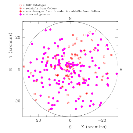
Figure 3: Coma galaxies observed (solid points) overlaid on the total sample defined in Section 2, i.e. galaxies with confirmed cluster membership and with $b_{j}\leq 18.0$.

5 Data reduction

5.1 Basic data reduction

The first step in the raw reduction was performed with the IRAF WYFFOS data reduction software (Pollacco et al. 1999). This software performs the following basic tasks: bias subtraction; aperture identification; scattered light correction; flat fielding; throughput correction; fibre extraction; wavelength calibration (using an Argon I lamp); and sky subtraction. Cosmic ray and night sky line removal were then performed using our own software. The wavelength calibration residuals had a median rms of 0.050 to 0.083 Å  for the three field configurations.

Individual spectra from a particular night were summed together to produce a spectrum of higher S/N. Where galaxies were observed on multiple nights it was decided not to co-add the spectra but rather treat each night as a separate measurement. This was because each spectra had sufficient S/N to yield high quality measurements without co-adding.

5.2 Redshift and velocity dispersion measurement

Velocity dispersions, $\sigma$ of the central 2.7^′′ region of a galaxy (determined by the fibre diameter, equivalent to 0.94 $h^{-1}$ kpc) are measured using the well-known Fourier Quotient method of Sargent et al. (1977). Recession velocities, $cz$, are obtained simultaneously with the velocity dispersions, as a result of the Fourier Quotient fit.

In the Fourier Quotient method a galaxy spectrum is approximated by the convolution of a representative stellar spectrum with an appropriate broadening function. This function is then calculated in Fourier parameter space. Prior to transforming to Fourier space, continuum fits are subtracted (using a 5th order polynomial) from both the stellar template spectrum and the galaxy spectrum, and modulated by a cosine bell function to fix the ends of the spectrum to zero. The latter step is necessary to avoid unphysical signals appearing at all frequencies in the Fourier transforms. These spectra then require filtering in Fourier space to remove signals arising from noise, inadequate continuum removal and the application of the cosine bell. A cut is made at high frequencies, to suppress channel-to-channel noise. The resulting $\sigma$ values are fairly insensitive to the exact value, $k_{\rm{high}}$, chosen for the high frequency cut. $k_{\rm{high}}=200$ has been used throughout. At low frequencies, a filter must be applied to remove residual continuum features and the effects of the cosine-bell modulation function described above. For the case of the low frequency cut, results are found to exhibit a clear trend: velocity dispersions are measured to be smaller when $k_{\rm{low}}$ is larger. The cut-off frequency must therefore be chosen with care. It is required that the low frequency filter should remove the signal arising from the cosine bell modulation, whilst preserving intrinsic features in spectra of velocity dispersion $\leq 500$ km s^-1. For the spectra herein, these constraints leave a range of $k_{\rm{low}}=6-9$ over which an average velocity dispersion is calculated.

In order for the recovered width to represent only the intrinsic velocity broadening of the galaxy spectrum, it is necessary to ensure that the stellar spectrum has been subject to the same instrumental resolution effects as the galaxy spectrum. This is done by observing standard stars throughout an observing run and comparing these spectra to the observed galaxy spectra. In this study, five radial velocity standard stars (stellar types G8iii to K3iii) were observed down a number of different fibres. Since these observed standard stars have small, but non-zero radial velocities it is necessary to first zero-redshift them. This is performed by applying the Fourier Quotient method to calculate the radial velocity of the standard stars against a high resolution (0.5 Å  per pixel), very high S/N ($\sim 250-1000$ per Å) spectrum that has been precisely zero-redshifted through the identification of spectral features and then shifting them to their laboratory rest frame. Four spectra were kindly supplied by Claire Halliday (private communication, hereafter referred to as the Halliday spectra). These allow the standard stars to be zero-redshifted to an accuracy of $\pm 6$ km s^-1.

Redshifts and velocity dispersions were measured both from each galaxy exposure and from the combined galaxy exposures for each night the galaxy was observed. The redshifts are corrected to heliocentric redshifts and the results averaged (weighting by their S/N) to yield a final value for a galaxy.

5.3 Spectral resolution variation

Using any multi-fibre spectroscopy instrument introduces intra-fibre and fibre-to-fibre variations in spectral resolution and throughput that necessarily have to be removed before an accurate analysis can be undertaken. These variations are due to the optical performance of the telescope plus instrumentation setup both across the field and along the slit where the fibres are fed into the spectrograph. These variations are found to be significant in the WHT/WYFFOS system and affect velocity dispersion and line-strength measurements (though to a lesser extent, see Section 6). In this section we describe how these variations are quantified.

The variation in spectral resolution was mapped by analysing the calibration spectra taken on each night. The arc lamps were located at the Cassegrain focus of the WHT and shine their light on to the tertiary mirror from which it is then relayed to the fibres. These allowed accurate mapping of the vignetting caused by the IDS grating H1800V convolved with a function representing the vignetting of the telescope optics from that point onwards. This approach is capable of removing the majority of the overall vignetting, since any effects superimposed by the telescope optics prior to the tertiary mirror are significantly smaller than the dominant effects subsequent to the tertiary mirror.

The results of this mapping can be seen in Fig. 4. A clear and sizable variation in spectral resolution is seen for each of the WYFFOS fibres. This effect is inherent in all telescopes due to the natural vignetting caused by their optical performance. However it is exacerbated in the WHT/WYFFOS system by the mis-match between the smaller IDS grating H1800V used and the larger WYFFOS beam; this mis-match further vignettes the spectra observed in fibres at the top and bottom ends of the slit. The widths of the Argon I calibration spectrum can be seen to vary from $\sim 4$ Å  at the end of the slit and at the edge of the field to $\sim 1.7$ Å  at the centre of the slit and at the centre of the field. This variation is a function both of fibre number (reflecting the position of the fibre on the slit and within the observed field) and of wavelength. These variations in line width will affect any velocity dispersion measurements (with a maximum error of 12 km s^-1 for $\sigma=100$ km s^-1), but will not change the redshift measurements (there is no systematic shift introduced by this problem) and will have a minor effect on line strengths (since the spectrum are broadened before measurement, see Section 7.2).

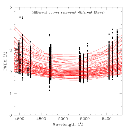
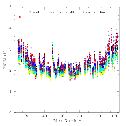
(a)	(b)

Figure 4: Dependence of Argon I emission line width on wavelength and fibre number. Fig. (a) shows the spectral resolution dependence on wavelength, whilst Fig. (b) shows the dependence on fibre number. Each point corresponds to a spectral line width measurement. Fig. (a) has a 2nd order polynomial fit to the spectral resolution variation with wavelength for each fibre superimposed. In Fig. (b) the points are shaded to indicate the different line width measurements for a fibre. See text for a more detailed explanation.

In principle it is possible that the variable throughput of the fibres might play a role here, with a dependence of spectral resolution on the strength of an arc line. However after further investigation this was ruled out. There could also be a further complication in that the tracking of the field centre on the Coma cluster during an exposure is not perfect, causing a drift in field position (and hence fibre position) relative to the target being observed. This drift, both during an exposure and between exposures, could introduce a time dependence into the mapping of the fibre characteristics. This effect was investigated by comparing the first and last spectra observed on a night and was found to be negligible ($\sim 0.1$ Å) compared to the other effects discussed.

6 Velocity dispersion corrections

6.1 Modelling the effect of intra–fibre and fibre–fibre variations

The first stage in removing the effect of any intra–fibre and fibre–fibre variations is to fit a function to the spectral resolution variation. We fit 2nd order polynomials to the variation with wavelength for each fibre and each field configuration (see Fig. 4a). These functions can then be convolved with an ideal template spectrum and the result used to cross-correlate against that of an observed galaxy to find its dispersion with any intrinsic fibre variation removed. The problem with this method is in having a template spectrum of very high resolution that is not itself suffering from any internal or instrumental variation.

To counter this problem we have devised the following method. We use the Halliday spectra which have been precisely zero-redshifted through the identification and then subsequent shifting of spectral features to their laboratory rest frame. These are the same spectra that were previously used to removed any redshift from observed standard stars in Section 5.2. These spectra will still suffer from some intrinsic variation (due to e.g. the telescope/instrument setup they were obtained with), but this is unimportant in the proposed method. These spectra are convolved with a particular fibre model in linear wavelength space, resulting in a ‘template spectrum’. The new template spectra are then cross-correlated against a mock galaxy created by convolving the original high-resolution spectra with a fibre model (not necessarily the same fibre) and broadening it by a fixed amount in logarithmic wavelength space (to simulate the Doppler broadening caused by a galaxy). A correction can then be calculated for each fibre configuration and each galaxy dispersion case:

$$\begin{array}[]{c}\rm{dispersion}\\ \rm{correction}\end{array}\quad=\quad\begin{array}[]{c}\rm{measured}\\ \rm{dispersion}\end{array}\quad-\quad\begin{array}[]{c}\rm{true}\\ \rm{dispersion}\end{array}$$ (1)

These corrections are then used to modify the real calculated dispersions which are calculated using template spectra observed on the night to cross-correlate against the galaxy spectra. This is done by subtracting the calculated correction from the measured value. In this way the ‘true’ (or best estimate) dispersion is derived, with any modifications due to intra–fibre and fibre–fibre variations removed. Some results of this method can be seen in Figs. 5 to 7.

Figure 5: Velocity dispersion measured versus galaxy fibre number for template stars observed with different fibres (template fibre numbers are given by the key at the top of the figure). Three plots are shown for the Halliday spectra broadened to 100, 200 and 300 km s^-1. The dashed line separate from the others corresponds to velocity dispersions measured versus a template star observed with fibre 14. This fibre suffers a large amount of spectral variation which greatly affects velocity dispersion measurements. See text.

Figure 6: Velocity dispersion correction versus galaxy fibre number for one template star observed with a particular fibre cross-correlated against a mock galaxy observed with different fibres and with various broadening factors (the different broadenings used are given by the key in the top right of the figure, these are 50–350 km s^-1). See text.

Figure 7: Velocity dispersion correction versus measured velocity dispersion for each fibre in a particular field setup cross-correlated against a standard star observed with a particular fibre (in this case fibre number 41). The curves are constructed by taking a Halliday spectrum, convolving it with a previously computed broadening function for a given fibre number and then broadening it by a given velocity dispersion from 25 to 350 km s^-1. This resultant mock galaxy spectra is then cross-correlated against a similar template spectra which has been convolved with a broadening function for a different fibre (matching a fibre number with which a standard star was observed during the run). The computed velocity dispersion is compared to the true velocity dispersion and a correction computed. A curve is then fit to the variation of the velocity dispersion correction with measured velocity dispersion. This curve (overlaid on the plot) can then subsequently used to correct an actual galaxy velocity dispersion measurement. Ideally all lines should be straight and coincident with a zero correction. See text.

Figs. 5 and 6 show the size of the velocity dispersion correction required versus galaxy fibre number for a range of template stars with different broadening factors (simulating the typical velocity dispersions of the observed galaxies) and different spectral resolution variation functions (simulating the variations introduced through observing a galaxy with different fibres). Ideally each plot should be a straight line, however this is not the case because of the WHT/WYFFOS spectral resolution variations. A correction therefore needs to be applied to the velocity dispersion measurements of the observed early-type galaxies. This correction is a function of the fibre number that the galaxy was observed with and of the fibre number that the star used for the velocity dispersion measurement was observed with. The size of the correction is also a function of the velocity dispersion of the galaxy observed (Fig. 7), with larger velocity dispersions requiring a smaller correction. These corrections are typically small, but where an unfavourable pairing between galaxy fibre and standard star fibre occurs the velocity dispersion correction can be as large as 20 km s^-1 for low velocity dispersion galaxies ($\sigma\simeq 50$ km s^-1). However for the typical velocity dispersions of the galaxies that we observed in this project ($\sigma\sim 100$ km s^-1 and greater) the corrections are not large, but are significant. As expected though, when a galaxy is cross-correlated against a standard star observed in the same field configuration and with the same fibre the velocity dispersion correction is zero.

This modelling of the effect of intra-fibre and fibre-fibre variations results in accurate velocity dispersions for the galaxies, which are subsequently required during the Lick/IDS stellar population index measurement process (see Section 7.6). Bootstrap tests on the accuracy of this method using the high-resolution, very high S/N stellar template spectra have shown that the random errors for the velocity dispersion corrections are $\sim 1-{2}$ km s^-1, demonstrating the success of this approach.

6.2 Redshift and velocity dispersion data

Table 7 lists the heliocentric redshift (135 galaxies) and central velocity dispersion data (132 galaxies) for the galaxies observed in the Coma cluster in this study. The dispersions have been corrected for the field variations (Section 5.3). These data are average values (weighted by their S/N) of all the measurements from the multiple exposures. Blank entries indicate a measurement was not possible.

The redshift errors are calculated by combining the error in the wavelength calibration in quadrature with the error resulting from the cross-correlation technique plus the template mis-matching error (calculated through cross-correlating the galaxy spectrum against different stellar spectra) and an additional error component factor (calculated from the variance between multiple exposures on a galaxy cross-correlated against a single stellar spectrum). The median heliocentric redshift error is 12 km s^-1.

The velocity dispersion errors are calculated by combining the error resulting from the cross-correlation technique in quadrature with the error resulting from template mis-matching (calculated through cross-correlating the galaxy spectrum against different stellar spectra) plus an additional error component factor (calculated from the variance between multiple exposures on a galaxy cross-correlated against a single stellar spectrum). The median velocity dispersion error is 0.015 dex.

Table 7: Heliocentric redshifts and central velocity dispersions.

name	type	S/N	cz⊙ (km s-1)	$\sigma$ (km s-1)
d26	S0p	53.5	7396 $\pm$ 12	71.5 $\pm$ 9.4
d27	E	41.3	7762 $\pm$ 12	107.4 $\pm$ 3.6
d28	E/S0	57.9	5974 $\pm$ 12	103.5 $\pm$ 4.5
d29	E	33.9	6973 $\pm$ 16	63.1 $\pm$ 8.6
d38	Sbc	38.8	5084 $\pm$ 12	71.3 $\pm$ 14.4
d39	S0/E	76.1	5897 $\pm$ 12	120.4 $\pm$ 3.4
d40	S0	47.0	5597 $\pm$ 12	72.9 $\pm$ 6.2
d42	S0	80.7	6016 $\pm$ 12	147.1 $\pm$ 7.0
d44	S0	55.7	7533 $\pm$ 12	55.4 $\pm$ 11.5
d50	SBa	38.4	5211 $\pm$ 11	54.0 $\pm$ 6.3
d53	E	80.2	5742 $\pm$ 12	128.4 $\pm$ 5.4
d57	S0/a	97.4	8384 $\pm$ 12	142.5 $\pm$ 4.7
d59	E	66.0	6947 $\pm$ 12	129.9 $\pm$ 5.0
d62	S0	51.9	8359 $\pm$ 16	126.2 $\pm$ 10.9
d63	S0/a	34.8	6675 $\pm$ 12	87.3 $\pm$ 4.8
d64	E	50.5	7010 $\pm$ 12	80.9 $\pm$ 5.6
d65	S0	65.1	6191 $\pm$ 12	116.3 $\pm$ 3.2
d67	S0	52.3	6039 $\pm$ 12	150.8 $\pm$ 2.0
d71	S0	42.3	6919 $\pm$ 12	63.9 $\pm$ 7.7
d73	E	49.2	5440 $\pm$ 12	73.5 $\pm$ 5.5
d74	E	27.9	5793 $\pm$ 11	41.1 $\pm$ 10.9
d75	S0	48.2	6132 $\pm$ 13	79.6 $\pm$ 5.8
d81	E	48.7	5928 $\pm$ 12	143.3 $\pm$ 2.3
d83	S0	31.3	8184 $\pm$ 12	37.5 $\pm$ 9.8
d84	S0	46.8	6553 $\pm$ 11	120.6 $\pm$ 3.5
d85	E	42.4	8251 $\pm$ 12	65.0 $\pm$ 5.8
d87	E	63.2	7770 $\pm$ 12	94.0 $\pm$ 4.7
d90	S0	52.0	5522 $\pm$ 12	88.5 $\pm$ 4.1
d93	S0	78.4	6063 $\pm$ 12	136.3 $\pm$ 4.9
d98	S0/a	77.7	6868 $\pm$ 12	130.0 $\pm$ 5.4
d107	E	39.3	6491 $\pm$ 12	87.7 $\pm$ 3.7
d108	S0	66.8	6424 $\pm$ 12	115.9 $\pm$ 3.2
d110	S0/E	60.3	6948 $\pm$ 12	114.4 $\pm$ 3.2
d112	E	50.8	7433 $\pm$ 13	58.3 $\pm$ 6.5
d116	SB0	75.7	8437 $\pm$ 12	123.2 $\pm$ 4.2
d117	S0/a	38.2	8561 $\pm$ 12	93.1 $\pm$ 4.8
d123	SB0	50.0	7712 $\pm$ 12	100.6 $\pm$ 3.3
d132	S0	46.7	7698 $\pm$ 12	96.2 $\pm$ 3.5
d134	E	63.7	7009 $\pm$ 12	126.7 $\pm$ 2.2
d135	E	36.8	8323 $\pm$ 12	100.2 $\pm$ 3.9
d136	E	82.0	5682 $\pm$ 11	168.8 $\pm$ 2.3
d142	E	79.0	7652 $\pm$ 12	161.4 $\pm$ 2.3
d147	S0	58.9	7713 $\pm$ 12	107.7 $\pm$ 3.9
d153	E	52.7	6684 $\pm$ 11	127.9 $\pm$ 2.7
d154	S0	51.1	6833 $\pm$ 11	57.1 $\pm$ 5.0
d156	E/S0	51.8	6671 $\pm$ 12	84.8 $\pm$ 7.9
d157	S0	74.8	6107 $\pm$ 12	131.5 $\pm$ 2.4
d158	S0	28.9	6058 $\pm$ 12	64.8 $\pm$ 6.1
d161	E	86.9	7146 $\pm$ 12	190.3 $\pm$ 4.9
d171	S0	81.0	6135 $\pm$ 12	127.5 $\pm$ 2.9
d181	S0	63.0	6090 $\pm$ 12	120.3 $\pm$ 4.5
d182	S0	44.0	5702 $\pm$ 12	120.2 $\pm$ 2.3
d191	S0	44.4	6592 $\pm$ 12	90.9 $\pm$ 5.2
d192	S0	56.4	5435 $\pm$ 12	87.5 $\pm$ 5.5
d193	E	72.4	7567 $\pm$ 12	117.6 $\pm$ 3.4
d200	S0	104.0	7466 $\pm$ 12	189.3 $\pm$ 4.5
d201	S0	36.5	6409 $\pm$ 12	59.6 $\pm$ 9.4
d204	E	53.1	7578 $\pm$ 12	126.1 $\pm$ 4.0
d207	E	78.1	6743 $\pm$ 12	146.9 $\pm$ 2.8
d209	S0	48.5	7182 $\pm$ 12	80.7 $\pm$ 5.2
d210	E	66.6	7252 $\pm$ 12	144.6 $\pm$ 3.8
d216	Sa	43.5	7684 $\pm$ 12	71.5 $\pm$ 13.0
d224	S0	42.2	7597 $\pm$ 12	59.5 $\pm$ 6.2

Table 8: continued

name	type	S/N	cz⊙ (km s-1)	$\sigma$ (km s-1)
d225	S0	38.1	5879 $\pm$ 14	71.7 $\pm$ 6.7
d231	S0	62.9	7878 $\pm$ 13	127.8 $\pm$ 5.0
ic3943	S0/a	97.8	6789 $\pm$ 12	168.6 $\pm$ 1.9
ic3946	S0	73.8	5927 $\pm$ 12	199.6 $\pm$ 2.6
ic3947	E	93.6	5675 $\pm$ 12	158.8 $\pm$ 2.1
ic3959	E	95.1	7059 $\pm$ 12	215.9 $\pm$ 6.0
ic3960	S0	95.5	6592 $\pm$ 12	174.3 $\pm$ 2.9
ic3963	S0	74.7	6839 $\pm$ 12	122.4 $\pm$ 3.9
ic3973	S0/a	78.3	4716 $\pm$ 12	228.0 $\pm$ 3.1
ic3976	S0	105.8	6814 $\pm$ 14	255.2 $\pm$ 6.4
ic3998	SB0	75.5	9420 $\pm$ 12	136.9 $\pm$ 4.9
ic4011	E	52.5	7253 $\pm$ 11	123.2 $\pm$ 3.6
ic4012	E	90.7	7251 $\pm$ 12	180.7 $\pm$ 3.7
ic4026	SB0	86.3	8168 $\pm$ 12	132.2 $\pm$ 3.0
ic4041	S0	76.6	7088 $\pm$ 12	132.5 $\pm$ 2.3
ic4042	S0/a	67.8	6371 $\pm$ 12	170.6 $\pm$ 3.3
ic4045	E	107.9	6992 $\pm$ 22	217.6 $\pm$ 3.6
ic4051	E	56.1	4994 $\pm$ 12	228.8 $\pm$ 2.5
ngc4848	Scd	46.7	7199 $\pm$ 16	106.8 $\pm$ 7.4
ngc4850	E/S0	105.6	6027 $\pm$ 12	189.8 $\pm$ 2.5
ngc4851	S0	50.0	7861 $\pm$ 12	126.8 $\pm$ 3.3
ngc4853	S0p	88.5	7676 $\pm$ 12	140.8 $\pm$ 4.4
ngc4860	E	76.6	7926 $\pm$ 12	277.3 $\pm$ 7.2
ngc4864	E	103.4	6828 $\pm$ 12	187.6 $\pm$ 3.2
ngc4867	E	117.3	4817 $\pm$ 12	208.5 $\pm$ 2.0
ngc4869	E	101.9	6844 $\pm$ 12	203.1 $\pm$ 4.4
ngc4872	E/S0	80.1	7198 $\pm$ 12	217.8 $\pm$ 3.4
ngc4873	S0	100.8	5818 $\pm$ 12	176.9 $\pm$ 1.8
ngc4874	cD	64.4	7180 $\pm$ 12	274.5 $\pm$ 3.3
ngc4875	S0	88.7	8014 $\pm$ 13	180.1 $\pm$ 4.3
ngc4876	E	82.0	6710 $\pm$ 12	164.1 $\pm$ 3.1
ngc4881	E	94.7	6730 $\pm$ 12	193.9 $\pm$ 4.9
ngc4883	S0	85.3	8161 $\pm$ 12	166.1 $\pm$ 2.7
ngc4886	E	41.7	6377 $\pm$ 12	153.8 $\pm$ 2.8
ngc4889	cD	141.6	6495 $\pm$ 13	397.5 $\pm$ 10.1
ngc4894	S0	55.0	4640 $\pm$ 12	85.6 $\pm$ 3.8
ngc4895	S0	106.9	8458 $\pm$ 15	239.8 $\pm$ 5.0
ngc4896	S0	67.7	5988 $\pm$ 18	164.0 $\pm$ 2.6
ngc4906	E	91.4	7505 $\pm$ 12	175.0 $\pm$ 4.4
ngc4907	Sb	56.8	5812 $\pm$ 12	148.2 $\pm$ 2.6
ngc4908	S0/E	72.5	8710 $\pm$ 12	193.9 $\pm$ 4.3
ngc4919	S0	121.0	7294 $\pm$ 12	191.5 $\pm$ 3.1
ngc4923	E	109.0	5487 $\pm$ 12	198.3 $\pm$ 3.5
rb58		22.6	7634 $\pm$ 12	50.1 $\pm$ 6.7
rb60		34.7	7895 $\pm$ 12	57.1 $\pm$ 6.8
rb66		30.7	5822 $\pm$ 11	43.0 $\pm$ 6.4
rb71		35.4	6839 $\pm$ 12
rb74	SA0	32.2	5899 $\pm$ 11	63.8 $\pm$ 4.8
rb94	SB0/a	28.7	5283 $\pm$ 12	57.6 $\pm$ 6.4
rb122		33.4	7082 $\pm$ 11	77.3 $\pm$ 6.3
rb128		36.0	7013 $\pm$ 12	150.3 $\pm$ 2.4
rb129	unE	58.2	5852 $\pm$ 12	89.9 $\pm$ 4.6
rb131		20.5	8209 $\pm$ 12	45.7 $\pm$ 11.3
rb153		22.9	6780 $\pm$ 12	51.6 $\pm$ 6.9
rb198	SA0	31.1	6177 $\pm$ 12	54.8 $\pm$ 5.7
rb199		21.2	8476 $\pm$ 46
rb223		64.0	6916 $\pm$ 12	94.4 $\pm$ 3.6
rb245		25.1	6009 $\pm$ 11	47.6 $\pm$ 6.1
gmp1986		13.3	6591 $\pm$ 12	22.8 $\pm$ 17.8
gmp2421		28.0	8132 $\pm$ 13	30.0 $\pm$ 38.6
gmp2688		30.1	7261 $\pm$ 12	58.8 $\pm$ 4.7
gmp2721		28.7	7580 $\pm$ 11	55.6 $\pm$ 5.4
gmp2783		22.6	5360 $\pm$ 12	39.8 $\pm$ 11.3

Table 9: continued

name	type	S/N	cz⊙ (km s-1)	$\sigma$ (km s-1)
gmp2942		47.1	7542 $\pm$ 12	149.9 $\pm$ 2.8
gmp3012		25.8	8041 $\pm$ 12	60.4 $\pm$ 8.2
gmp3298		28.5	6786 $\pm$ 12	51.3 $\pm$ 8.3
gmp3585		29.5	5178 $\pm$ 22	52.8 $\pm$ 23.1
gmp3588		24.1	6033 $\pm$ 13	55.5 $\pm$ 7.2
gmp3829		18.6	8577 $\pm$ 12	48.4 $\pm$ 5.0
gmp4348		29.2	7581 $\pm$ 12	56.3 $\pm$ 18.8
gmp4420		40.6	8520 $\pm$ 13	59.6 $\pm$ 12.0
gmp4469		15.8	7467 $\pm$ 12

Notes: These results are average values (weighted by their S/N) of all of the measurements from the multiple exposures. Blank entries indicate a measurement was not possible. There are a total of 135 galaxies in this data table. Morphological types are taken from Dressler (1980a). S/N is measured at the centre of index Fe5270.

7 Stellar population absorption line strengths

One of the main goals of this study was to measure the luminosity weighted mean ages and metallicities of the dominant stellar populations within the core of bright early-type galaxies. To measure these ages and metallicities, we used the Lick/IDS system of line strength measurement and then compared the data to models (e.g. Worthey 1994). The principal line indices used were H$\beta_{\rm{G}}$ (predominantly age dependent) and $[$MgFe$]$ (predominantly metallicity dependent). This section details the measurement of these and other stellar population absorption line strength indices in the wavelength range $\sim$4600–5600 Å.

7.1 Flux calibration

It is first necessary to remove the overall instrument response function (IRF) from galaxy spectra prior to line strength measurement. Spectra are affected by: the response of the spectrograph optics; the response of the CCD; the response of the grating; atmospheric conditions; and airmass. These effects are removed by observing flux standard stars (see e.g. Massey et al. 1988). Flux calibration of the galaxy spectra was performed by comparing the observed stars to their standard spectrum and computing the IRF which was then used to transform the galaxy spectra continuum. Since the conditions these observations were performed in were not photometric, it is only possible to correct the galaxy spectra to some arbitrary flux units. However this does not affect the shape of the spectral continuum nor the line strength measurements. To improve the calculation of the IRF a number of flux standard stars were observed during the run. The IRFs calculated from each star were then compared and a mean IRF derived using a technique that minimized their maximum absolute deviations (MAD).

It was not possible to measure flux standard stars down each fibre and for each field configuration because of the prohibitively long observing time required. This means that the computed IRF function is only an overall IRF and does not include fibre-to-fibre continuum shape variations. This fibre-to-fibre IRF variation is however small and would only affect line strength measurements at the level of $<0.1$ Å.

A typical flux calibrated galaxy spectrum is shown in Fig. 8.

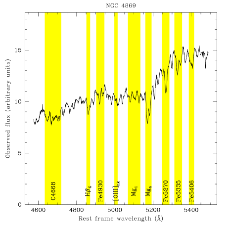
Figure 8: Fluxed spectrum of galaxy NGC 4869 shifted to its rest frame wavelength. The Lick/IDS features present in the spectrum are shaded.

7.2 Lick/IDS system

Absorption line strengths were measured using the Lick/IDS system of indices, where a central feature bandpass is flanked on either side by pseudo-continuum bandpasses (see Trager et al. 1998 for details). The Lick/IDS system is based upon spectra with a mean resolution of 9 Å  (Fig. 9). The spectra in this study need to be broadened to the same resolution to measure indices on the Lick/IDS system. This is done by calculating a transformation function using the known resolution function of a galaxy spectrum (Section 5.3) and the Lick/IDS resolution function (see Fig. 9 or Worthey & Ottaviani 1997):

$${\rm{FWHM}}_{trans}(\lambda)^{2}={\rm{FWHM}}_{Lick}(\lambda)^{2}-{\rm{FWHM}}_{gal}(\lambda)^{2}$$ (2)

The spectrum is then broadened in linear wavelength space using a sliding Gaussian smoothing function derived from this transformation function.

Figure 9: Comparison of the variation in FWHM with wavelength for this study and for the Lick/IDS system. The mean resolution of this study is $\sim$2.2 Å  (see Fig. 4), whereas the mean resolution of the Lick/IDS system is 9 Å. This Lick/IDS resolution varies to values 30 per cent higher at the ends of the spectra. To measure line strengths on the Lick/IDS system it is necessary to broaden any higher resolution spectra to the same resolution (Worthey & Ottaviani 1997).

7.3 Line strength measurement

Indices were measured by first zero-redshifting galaxy spectra to the laboratory rest frame using the previously measured heliocentric redshifts corrected back to the geocentric rest frame. Then the mean height in each of the two pseudo-continuum regions was determined in either side of the feature bandpass, and a straight line drawn through the mid-point of each one. The difference in flux between this line and the observed spectrum within the feature bandpass determines the index. For narrow features, the indices are expressed in angstroms (Å) of equivalent width (EW); for broad molecular bands, in magnitudes. Specifically, the average pseudo-continuum flux level is:

$$F_{P}=\int_{\lambda_{1}}^{\lambda_{2}}\frac{F_{\lambda}}{(\lambda_{2}-\lambda_{1})}d\lambda$$ (3)

where $\lambda_{1}$ and $\lambda_{2}$ are the wavelength limits of the pseudo-continuum sideband. If $F_{C\lambda}$ represents the straight line connecting the midpoints of the blue and red pseudo-continuum levels, an equivalent width is then:

$$\rm{EW}=\int_{\lambda_{1}}^{\lambda_{2}}\left(1-\frac{F_{I\lambda}}{F_{C\lambda}}\right)d\lambda$$ (4)

where $F_{I\lambda}$ is the observed flux per unit wavelength and $\lambda_{1}$ and $\lambda_{2}$ are the wavelength limits of the feature passband. Similarly, an index measured in magnitudes is:

$$\rm{mag}=-2.5\log_{10}\left[\left(\frac{1}{\lambda_{2}-\lambda_{1}}\right)\int_{\lambda_{1}}^{\lambda_{2}}\frac{F_{I\lambda}}{F_{C\lambda}}d\lambda\right]$$ (5)

These definitions, after Trager et al. (1998), differ slightly from those used in Burstein et al. (1984) and Faber et al. (1985) for the original 11 IDS indices. In the original scheme, the continuum was taken to be a horizontal line over the feature bandpass at the level $F_{C\lambda}$ taken at the midpoint of the bandpass. This flat rather than sloping continuum would induce erroneous small, systematic shifts in the feature strengths.

An example of the measurement of the Mg_b index for galaxy NGC 4869, an elliptical galaxy with $b_{j}=14.97$ and $\sigma=203$ km s^-1, is shown in Fig. 10.

Figure 10: Measurement of Mg_b index for galaxy NGC 4869 (an elliptical galaxy with $b_{j}=14.97$ and $\sigma=203$ km s^-1). The fluxed spectrum at rest wavelength is overlaid with the spectrum transformed to the Lick/IDS system spectral resolution (solid line). The two pseudo-continuum bandpasses are marked either side of the Mg_b feature (also marked); the mean level at the mid-point of the two pseudo-continuum bandpasses are joined by a straight line and the flux in the index feature relative to this line computed.

7.4 Indices measured

Table 10 presents the stellar population absorption line indices measured in this work. Column (5) is after the work of Tripicco & Bell (1995), who modelled the Lick/IDS system using synthetic stellar spectra. They found that many of the Lick/IDS indices do not in fact measure the abundances of the elements for which they are named. The following composite indices were also measured in our study:

$$\langle\rm{Fe}\rangle=\frac{\rm{Fe5270}+\rm{Fe5335}}{2}$$ (6)

$$[\rm{MgFe}]=\sqrt{\rm{Mg}_{\rm{b}}\,\times\,\langle\rm{Fe}\rangle}$$ (7)

Table 10: Stellar population analysis spectral line index definitions.

Name	Index Bandpass (Å)	Pseudocontinua (Å)	Units	Measures	Source
(1)	(2)	(3)	(4)	(5)	(6)
C4668†	4634.000–4720.250	4611.500–4630.250	Å	C,(O),(Si)	Lick
		4742.750–4756.500
H$\beta$	4847.875–4876.625	4827.875–4847.875	Å	H$\beta$,(Mg)	Lick
		4876.625–4891.625
Fe5015	4977.750–5054.000	4946.500–4977.750	Å	(Mg),Ti,Fe	Lick
		5054.000–5065.250
Mg1	5069.125–5134.125	4895.125–4957.625	mag	C,Mg,(O),(Fe)	Lick
		5301.125–5366.125
Mg2	5154.125–5196.625	4895.125–4957.625	mag	Mg,C,(Fe),(O)	Lick
		5301.125–5366.125
Mgb	5160.125–5192.625	5142.625–5161.375	Å	Mg,(C),(Cr)	Lick
		5191.375–5206.375
Fe5270	5245.650–5285.650	5233.150–5248.150	Å	Fe,C,(Mg)	Lick
		5285.650–5318.150
Fe5335	5312.125–5352.125	5304.625–5315.875	Å	Fe,(C),(Mg),Cr	Lick
		5353.375–5363.375
Fe5406	5387.500–5415.000	5376.250–5387.500	Å	Fe	Lick
		5415.000–5425.000
H$\beta_{\rm{G}}$	4851.320–4871.320	4815.000–4845.000	Å	H$\beta$,(Mg)	González (1993), p116
		4880.000–4930.000			Jørgensen (1997)
Fe4930	4903.000–4945.500	4894.500–4907.000	Å	Fe I,Ba II,Fe II	González (1993), p34
		4943.750–4954.500
$[$Oiii$]$1	4948.920–4978.920	4885.000–4935.000	Å	$[$Oiii$]$	González (1993), p116
		5030.000–5070.000
$[$Oiii$]$2	4996.850–5016.850	4885.000–4935.000	Å	$[$Oiii$]$	González (1993), p116
		5030.000–5070.000
$[$Oiii$]$hk	4998.000–5015.000	4978.000–4998.000	Å	$[$Oiii$]$	Kuntschner (2000)
		5015.000–5030.000
Notes: †Worthey (1994) called this index Fe4668. In publications after 1995 this index is called C24668
since it turned out to depend more on carbon than on iron.

7.5 Signal-to-noise

Our goal was to measure high signal-to-noise (S/N) line strength indices to probe the age and metallicity structure of the Coma cluster early-type galaxy population. We therefore measured a S/N at the central rest wavelength of each line index investigated in this study. The line indices H$\beta_{\rm{G}}$ and $[$MgFe$]$ have a mean S/N for their combined exposures of 58.7 and 66.7 per Å  respectively if a minimum cut-off of S/N$\geq$35 per Å  is applied. This minimum S/N cut-off is chosen to keep the errors of the line indices small in subsequent stellar population analyses. Fig. 11 shows the distribution of S/N for our sample as measured at the H$\beta_{\rm{G}}$ index.

(a) combined exposures only	(b) individual and combined
	exposures

Figure 11: A histogram of the S/N per Å  of the stellar population absorption line index H$\beta_{\rm{G}}$ measured from each galaxy spectrum. The bold vertical line indicates a S/N of 35 per Å.

7.6 Line index velocity dispersion correction

The observed spectrum of a galaxy is the convolution of the integrated spectrum of its stellar population with the instrumental broadening and the distribution of line-of-sight velocities of the stars (parameterized by the velocity dispersion measurement). The broadening of the spectra generally causes the indices to appear weaker than they intrinsically are.

To probe the stellar population of a galaxy it is necessary to remove the effects of the instrumental and velocity dispersion broadening. This gives an index measurement corrected to zero velocity dispersion. This was done by using the spectra of standard stars that were observed during the run. These stellar spectra were convolved in logarithmic wavelength space with a Gaussian function of widths 0–460 km s^-1 (in steps of 20 km s^-1) to simulate the velocity dispersion broadening within a galaxy. They were then converted in linear wavelength space to the Lick/IDS resolution using the method detailed in Section 7.2. Index strengths were measured for each spectrum. These values were compared to the values measured from the zero velocity dispersion stellar spectra which have also been transformed to the Lick/IDS resolution. A correction function versus velocity dispersion for each line index was then computed by calculating the difference between the broadened value and the zero velocity dispersion value and then dividing it by the zero velocity dispersion value. For each line index, a second order polynomial was fit to the correction function data from all the observed standard stars. This function was then evaluated at the velocity dispersion of each observed galaxy and the measured line index value for that galaxy corrected to a zero velocity dispersion value. After Kuntschner (2000), stars with low H$\beta$ ($<1.6$ Å) which are unrepresentative of bright elliptical galaxies are excluded from the analysis.

The correction functions for the line indices Mg_b and H$\beta_{\rm{G}}$ are shown in Fig. 12. Table 11 gives the polynomial coefficients for each line index correction function and the size of the correction for a galaxy with a velocity dispersion, $\sigma$ of 200 km s^-1. The corrections are multiplicative except for the Mg₁ and Mg₂ indices where the corrections are additive (since they are measured in magnitudes rather than in equivalent widths).

Table 11: Velocity dispersion correction polynomial coefficients.

				Correction
	correction = a0 + a1.$\sigma$ + a2.$\sigma^{2}$			at $\sigma$ =
Index	a0	a1	a2	200 km s-1
C4668	9.994e–01	–5.779e–06	9.102e–07	$\times$ 1.035
Fe4930	9.945e–01	1.087e–04	4.743e–06	$\times$ 1.206
Fe5015	9.893e–01	3.144e–04	1.494e–06	$\times$ 1.112
Fe5270	9.914e–01	2.538e–04	1.553e–06	$\times$ 1.104
Fe5335	1.001e+00	–7.494e–05	5.355e–06	$\times$ 1.200
Fe5406	1.007e+00	–2.662e–04	5.744e–06	$\times$ 1.184
H$\beta$	1.003e+00	–6.225e–05	7.326e–07	$\times$ 1.020
H$\beta_{\rm{G}}$	9.994e–01	–1.935e–05	1.007e–06	$\times$ 1.036
Mg1	–4.380e–04	1.154e–05	2.233e–08	$+$ 0.0028
Mg2	2.811e–05	1.888e–06	3.147e–08	$+$ 0.0017
Mgb	9.963e–01	4.038e–05	2.034e–06	$\times$ 1.086

Notes: The final column gives the correction for a $\sigma=200$ km s^-1 galaxy as an example of the scale of the correction necessary.

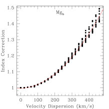
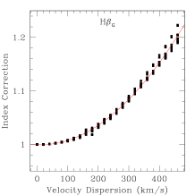
Figure 12: Velocity dispersion correction functions for the Mg_b and H$\beta_{\rm{G}}$ line indices. Each point corresponds to an index correction calculated from broadening an observed star and comparing the index measured from that spectrum to that from the unbroadened spectrum. The second order polynomial fit to the data is superimposed on the plot.

7.7 Emission correction

An important issue when estimating ages and metallicities from line strength indices is nebular emission. Elliptical galaxies normally contain much less dust and ionized gas than spirals, and were regarded as dust and gas free for a long time. Surveys of large samples of early type galaxies (Phillips et al. 1986; Caldwell 1984; Goudfrooij et al. 1994) have revealed however that 50–60 per cent of the galaxies show weak optical emission lines. The measured emission line strengths of [Oii], [H$\alpha$] and [Nii]$\lambda$6584 indicate a presence of only 10³–10${}^{5}{\rm{M}}_{\odot}$ of warm ionized gas in the galaxy centre. Additionally, HST images of nearby bright early type galaxies revealed that approximately 70–80 per cent show dust features in the nucleus (van Dokkum & Franx 1995). Stellar absorption line strength measurements can be severely affected if there is emission present in the galaxy (e.g. González 1993; Goudfrooij & Emsellem 1996): nebular H$\beta$ emission on top of the integrated stellar H$\beta$ absorption weakens the H$\beta$ index and leads therefore to incorrectly older age estimates.

In the González (1993) study of bright elliptical galaxies in groups and clusters, he noted that [Oiii] emission at 4959 Å  and 5007 Å  are clearly detectable in about half of the nuclei in his sample and that most of these galaxies also have detectable H$\beta$ emission (see his Fig 4.10). For galaxies in his sample with strong emission, H$\beta$ is fairly tightly correlated with [Oiii] such that:

$$\frac{\rm{H}\beta\;\rm{emission}}{[\rm{O\sc{iii}}]}\sim 0.7$$ (8)

A statistical correction of:

$$\Delta\rm{H}\beta\,=\,0.7\,[\rm{O\sc{iii}}]$$ (9)

was therefore added to H$\beta$ to correct for this residual emission.

Trager et al. (2000a,b) re-examined the accuracy of this correction by studying H$\beta$/[Oiii] among the González (1993) galaxies, supplemented by additional early type galaxies from the emission line catalogue of Ho, Filippenko & Sargent (1997). The sample was restricted to include only normal, non-AGN Hubble types E through to S0 and well measured objects with H$\alpha>1.0$ Å. For 27 galaxies meeting these criteria, they found that H$\beta$/[Oiii] varies from 0.33 to 1.25, with a median value of 0.60. They suggest that a better correction coefficient in Equation (9) is 0.6 rather than 0.7:

$$\Delta\rm{H}\beta\,=\,0.6\,[\rm{O\sc{iii}}]$$ (10)

implying that the average galaxy in the González (1993) sample is slightly over-corrected. For a median [Oiii] strength through the González (1993) $r_{e}/8$ aperture of 0.17 Å, the error due to this correction difference would be 0.02 Å  or $\sim$3 per cent in age. This systematic error for a typical galaxy is negligible compared to other sources of error.

In this study we adopt the 0.6 multiplicative factor to correct the H$\beta$ index for nebular emission using the [Oiii]$\lambda$5007 Å  emission line strength. Whilst there is evidence that this correction factor is uncertain for individual galaxies (Mehlert et al. 2000), it is good in a statistical sense for the study sample. After Kuntschner (2000), we adopt a slightly different definition of the [Oiii] emission line strength index bandpasses which we have found better measures the true [Oiii] emission. After the Lick/IDS system of measuring line indices, we define the feature bandpass to be 4998–5015 Å  and the continuum side bandpasses to be 4978–4998 Å  and 5015–5030 Å. This new definition does not affect the conclusions of Trager et al. (2000a,b) nor González (1993) on the relationship of [Oiii] to H$\beta$ emission. To further improve the measurement of the [Oiii] emission line strength in this study, we measure our best estimate of the emission by first subtracting a zero emission template from a galaxy spectrum and then measuring the residual equivalent width. The zero emission template is simply a standard star. The process is repeated for a set of zero emission templates and an average [Oiii] emission line strength calculated. An example of this process is shown in Fig. 13.

Figure 13: Example of our [Oiii]$\lambda$5007 Å  emission line strength measurement. Galaxy NGC 4850, type E/S0, is shown. The top part of the figure shows the fluxed galaxy spectrum (arbitrary units) overlaid with a zero emission template (thick line) whose continuum has been matched to the galaxy by minimising the maximum absolute deviation between the two spectrum. The vertical line marks the centre of the [Oiii]$\lambda$5007 Å  feature, whilst the dashed horizontal bar at the very top marks the continuum side bandpasses and width of the feature. The bottom part of the figure shows the difference between the galaxy and the zero emission template (a standard star) overlaid with the difference broadened to the Lick resolution (thick line). The spectrum shows clear [Oiii]$\lambda$5007 Å  emission.

A total of 50 galaxies were found to have 1 sigma evidence of [Oiii]$\lambda$5007 Å  emission, with a median emission of 0.228 Å  giving a median H$\beta$ correction of 0.137 Å  (see Fig. 14). The H$\beta$ correction is calculated separately for each galaxy using Equation (10) and our best estimate of the [Oiii]$\lambda$5007 Å  emission for that galaxy.

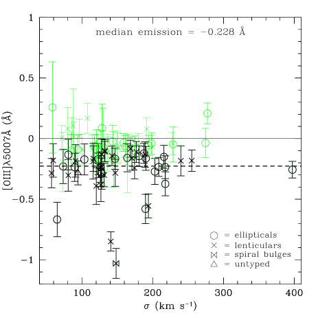
Figure 14: Summary of [Oiii]$\lambda$5007 Å  emission line strength measurements. A total of 50 galaxies (shown in a darker shade on the graph) were found to have 1 sigma evidence of [Oiii]$\lambda$5007 Å  emission, with a median emission of 0.228 Å  (marked as a bold dashed line on the graph) giving a median H$\beta$ correction of 0.137 Å. The H$\beta$ correction is calculated separately for each galaxy using Equation (10) and our best estimate of the [Oiii]$\lambda$5007 Å  emission for that galaxy.

7.8 Line strength index errors

The line index measurement errors were calculated by internal comparison during a night and between nights. With the large amount of multiple observations with different fibre configurations and high S/N data this allows accurate mapping of the random and some of the systematic errors.

The method assumes that the errors have an underlying Gaussian nature and exploits the central limit theorem. Firstly it is necessary to compute the difference between the multiple line index measurements taken during a night to the ‘true’ line index measurement, taken to be the measurement from the combined exposure for that night. To prevent any contaminating systematics, only exposures from a particular night were compared. In this way we mapped the random errors as a function of galaxy S/N up to a maximum S/N governed by the individual exposures. To extend this random error mapping to a higher S/N limit, we used the fact that a number of galaxies were observed every night during the observing run and further compared the line index measurement from the combined exposure for a night to the mean line index measurement from all of the nights, taken here to be the ‘true’ measurement as before. This mapping to higher S/Ns is only done for galaxies observed on all nights (often with different fibres due to the different field fibre configurations) to minimize any systematic error contamination of the random error mapping.

Once we obtained the dependence of the random errors with S/N for a particular line index, we deduced the error function for that index. The error function is calculated by binning the data by S/N from 5–35 S/N per Å  with bin widths of 3 S/N per Å  (the lower limit is to exclude very low S/N spectra which would contaminate the derivation of the error function). These bins were then analysed and a standard deviation computed for each bin. For spectra with a S/N greater than 35 per Å  binning is no longer used to prevent contamination by small number statistics. Instead a standard deviation was computed for the differences for all galaxies with a S/N greater than 35 per Å  and then this lower limit was incremented by the bin width and the standard deviation re-computed. This process was repeated up to a maximum S/N of 120 per Å. This procedure results in a data set of standard deviation versus S/N. A 4th order polynomial was then fit to the natural log of the variation of standard deviation with S/N (the function is fit to the natural logarithm of the data to simply fit a smoother function to the data, without introducing any erroneous high order fluctuations). Fig. 15 shows the error calculation plots for the Mg_b and H$\beta_{\rm{G}}$ line indices.

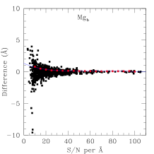
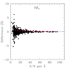
Figure 15: Error calculation plots for the Mg_b and H$\beta_{\rm{G}}$ line indices.

The computed error function versus S/N was subsequently used to calculate the errors for all of the line index measurements.

Table 12: Summary of error calculation results.

		Median	Systematic	Scale test
Index	Ngals	error	error	result
C4668	75	0.638 Å	–0.007 Å	1.052
Fe4930	97	0.160 Å	–0.002 Å	1.047
Fe5015	101	0.729 Å	–0.001 Å	0.892
Fe5270	109	0.136 Å	–0.002 Å	1.062
Fe5335	109	0.180 Å	0.002 Å	1.007
Fe5406	54	0.118 Å	–0.000 Å	1.647
H$\beta$	95	0.106 Å	–0.002 Å	1.104
H$\beta_{\rm{G}}$	95	0.103 Å	–0.001 Å	1.042
$\langle$Fe$\rangle$	109	0.114 Å	0.002 Å	1.035
Mg1	103	0.0090 mag	–0.0002 mag	0.904
Mg2	102	0.0066 mag	–0.0001 mag	0.953
Mgb	103	0.123 Å	0.000 Å	1.033
$[$MgFe$]$	109	0.085 Å	–0.006 Å	1.034
$[$Oiii$]$1	99	0.203 Å	0.001 Å	0.979
$[$Oiii$]$2	101	0.122 Å	0.003 Å	1.026
$[$Oiii$]$hk	93	0.075 Å	–0.002 Å	1.048

Notes: Median errors for all data with a S/N$\geq$35 per Å  are shown. The results of an internal systematic error analysis and of the scale test check are also included (see text). There are no internal systematic errors during a night nor between nights. The only significant scale test result is that for Fe5406; this result implies that the median error should be 0.194 Å.

To test the correctness of the error determination the central limit theorem was exploited to perform a scale test on the data. If the errors computed are appropriate then the following function will have a standard deviation equal to unity:

$$\begin{array}[]{c}\rm{scale\;test}\\ \rm{parameter}\end{array}\quad=\quad\frac{\begin{array}[]{c}\rm{line\;index}\\ \rm{measurement}\end{array}\/-\/\begin{array}[]{c}\rm{true\;line}\\ \rm{index\;value}\end{array}}{\begin{array}[]{c}\rm{line\;index}\\ \rm{error}\end{array}}$$ (11)

This scale test was performed on all data with a S/N greater than 10 per Å  to prevent any contamination by very low S/N measurements. In our case the true line index value is equal to the mean line index value. It is therefore necessary to include the error on the mean in the line index error. Table 12 includes the results of the scale test for each line index measured. The scale test parameter does indeed have a standard deviation approximately equal to unity (apart from the Fe5406 index), showing that the errors calculated are truly representative. For the Fe5406 index, the scale test implies that the median error should be 0.194 Å. A possible explanation for the difference between our error estimate and the conclusion of the scale test is the proximity of the index to the end of the wavelength range. In a conservative approach we adopt a final error for Fe5406 scaled by a factor 1.647.

In addition to the scale test, we conducted an internal systematic error analysis. A mean difference was calculated for data with a S/N$\geq$10 per Å  (the same low S/N cut-off used in the scale test), however only the central 68.3 per cent of this sample (i.e. 1 sigma clipping) were used so that effect of any rogue outliers in the sample distribution was minimized. The conclusion of this analysis was that there are no internal systematic errors either during a night or between nights.

7.9 Lick/IDS index absorption line strength data

Table 16 lists the Lick/IDS index absorption line strength data for 132 galaxies observed in the Coma cluster in this study. The three remaining galaxies (RB 71, RB 199, GMP 4469) had insufficient S/N to permit any line strength measurement. Missing values in the table indicate either that the line strength measured had a low S/N or that it could not be measured. Where a galaxy was observed on multiple nights with the same wavelength range, the line strength measurements from each night were combined using the square of the S/N to weight the measurements. The H$\beta$ and H$\beta_{\rm{G}}$ line strengths given in the table have not been corrected for nebula emission. The [Oiii]$\lambda$5007 Å  emission line strength measurement used for this correction is in the column $[$Oiii$]$_sm.

8 Comparison with previous data

Although the spectral resolution of the Lick/IDS system has been well matched, small systematic offsets in the indices introduced by continuum shape differences are generally present (note that the original Lick/IDS spectra are not flux calibrated). These offsets do not depend on the velocity dispersion of the galaxy itself. To establish these offsets we compared our measurements with data from studies that have galaxies in common:

(i)   Seven Samurai (Dressler et al. 1987; Faber et al. 1987);
(ii)  Lick/IDS database (Trager et al. 1998);
(iii) Jørgensen (1999);
(iv)  SMAC (Hudson et al. 2001);
(v)   Mehlert et al. (2000);
(vi)  Kuntschner et al. (2001).

Whilst some of the above studies partly contain data from the same source, for simplicity they are treated as independent studies.

This comparative analysis investigated the following hypothesis: an offset could be present between the data in this study and the published data sets, but there should be no offset between each of the comparison sets (since these have already been corrected to a common Lick/IDS system). This analysis also allowed a direct comparative measure of the quality of the data in this study.

8.1 Method of analysis

The following statistics were calculated for each sample of data from this study (with S/N$\geq$35 per Å) that matches with that of a previous study:

(i)   mean offset to this study;
(ii)  root mean squared of sample differences (rms);
(iii) intrinsic root mean squared of sample differences, taking into account the measurement errors (rms_intr).

All offsets were calculated as:

$$\rm{offset}\quad=\quad\begin{array}[]{c}\rm{data\;from}\\ \rm{this\;study}\end{array}\quad-\quad\begin{array}[]{c}\rm{data\;from\;a}\\ \rm{comparison\;study}\end{array}$$ (12)

The intrinsic root mean squared of sample differences is a test of the quality of the data errors: if the quoted errors on the parameters are correct, then the intrinsic rms should be negligible (i.e. close to zero).

8.2 Results of comparisons

Table 13 shows the results of the comparisons between the data in this study with that in previous studies. Intrinsic scatters are not calculated for the Seven Samurai data (Dressler et al. 1987) because they do not quote individual measurement errors.

Our velocity dispersion measurements show good agreement with published values, with the mean offsets all being less than 3 per cent (see Fig. 16). After allowing for the quoted measurement errors, only a small intrinsic scatter of 0.0216 dex is seen. To remove this intrinsic scatter the quoted measurement errors have to be increased by only $\sim 15$ per cent. These velocity dispersions will be used in Paper III with photometric data to investigate various spectro-photometric relations, using the stellar population parameters to probe their fundamental nature

Figure 16: Comparison between the velocity dispersions in this study and those from other studies of the Coma cluster. The difference is calculated as the data from this study minus the data from a comparison study. The plots at the top of the figure break down the comparison, showing the matching data between this study and each of the matching studies. The plot at the bottom of the figure shows the total data set used for the comparative analysis. The horizontal dashed lines indicate the mean offset and a median error bar is shown.

Table 13: Comparison between this study and other studies of the Coma cluster.

Data	S	N	Offset	rms	rmsintr
$\log\sigma$	7	23	0.0093$\pm$0.0081	0.0379
$\log\sigma$	S	33	0.0115$\pm$0.0078	0.0443	0.0222$\pm$0.0039
$\log\sigma$	J	18	–0.0037$\pm$0.0075	0.0308	0.0158$\pm$0.0037
$\log\sigma$	H	14	0.0059$\pm$0.0121	0.0437	0.0231$\pm$0.0062
$\log\sigma$	A	88	0.0070$\pm$0.0043	0.0405	0.0216$\pm$0.0027†
C4668	L	9	0.783$\pm$0.272	0.770	0.383$\pm$0.128
Fe5015	L	11	0.006$\pm$0.192	0.609	0.532$\pm$0.160
Fe5270	L	11	–0.026$\pm$0.147	0.464	0.065$\pm$0.020
Fe5335	L	10	0.329$\pm$0.135	0.405	0.129$\pm$0.041
Fe5406	L	5	0.134$\pm$0.245	0.491	0.097$\pm$0.044
$\langle$Fe$\rangle$	J	36	–0.121$\pm$0.050	0.294	0.046$\pm$0.008
$\langle$Fe$\rangle$	H	14	0.121$\pm$0.084	0.304	0.090$\pm$0.024
$\langle$Fe$\rangle$	L	10	0.204$\pm$0.050	0.150	0.183$\pm$0.058
$\langle$Fe$\rangle$	M	18	0.157$\pm$0.039	0.159	0.050$\pm$0.012
$\langle$Fe$\rangle$	A	78	0.028$\pm$0.033	0.291	0.048$\pm$0.005
Mg1	J	36	0.0203$\pm$0.0026	0.0152	0.0040$\pm$0.0007
Mg1	L	11	0.0208$\pm$0.0073	0.0219	0.0075$\pm$0.0024
Mg1	A	47	0.0204$\pm$0.0025	0.0169	0.0050$\pm$0.0007
Mg2	7	23	–0.0063$\pm$0.0036	0.0169
Mg2	S	33	0.0051$\pm$0.0029	0.0164	0.0094$\pm$0.0017
Mg2	J	36	0.0024$\pm$0.0033	0.0198	0.0099$\pm$0.0017
Mg2	H	14	0.0157$\pm$0.0059	0.0204	0.0111$\pm$0.0031
Mg2	L	11	0.0221$\pm$0.0073	0.0232	0.0087$\pm$0.0026
Mg2	A	117	0.0048$\pm$0.0019	0.0205	0.0111$\pm$0.0012†
Mgb	J	36	0.015$\pm$0.053	0.312	0.036$\pm$0.006
Mgb	H	14	0.180$\pm$0.062	0.222	0.012$\pm$0.003
Mgb	L	11	0.007$\pm$0.135	0.426	0.002$\pm$0.001
Mgb	M	18	0.132$\pm$0.068	0.279	0.034$\pm$0.008
Mgb	A	79	0.070$\pm$0.036	0.318	0.035$\pm$0.004
$[$MgFe$]$	J	36	–0.143$\pm$0.039	0.229	0.044$\pm$0.007
$[$MgFe$]$	H	14	0.148$\pm$0.067	0.240	0.081$\pm$0.022
$[$MgFe$]$	L	10	0.158$\pm$0.080	0.238	0.031$\pm$0.010
$[$MgFe$]$	M	18	0.152$\pm$0.040	0.165	0.004$\pm$0.001
$[$MgFe$]$	A	78	0.016$\pm$0.030	0.264	0.078$\pm$0.009
H$\beta$	J	35	–0.210$\pm$0.059	0.345	0.085$\pm$0.014
H$\beta$	H	13	0.194$\pm$0.102	0.354	0.139$\pm$0.038
H$\beta$	L	10	–0.005$\pm$0.148	0.443	0.091$\pm$0.029
H$\beta$	M	18	–0.099$\pm$0.067	0.276	0.051$\pm$0.012
H$\beta$	A	76	–0.088$\pm$0.043	0.376	0.120$\pm$0.014
H$\beta_{\rm{G}}$	J	35	–0.106$\pm$0.055	0.321	0.129$\pm$0.022

Notes: The different sources, S used for comparison are given by the key below:

7 = 7S	= Seven Samurai studies (Dressler et al. 1987)
S = SMAC	= Streaming Motions of Abell Clusters
	(Hudson et al. 2001)
J = Jørg	= Jørgensen (1999)
H = HK	= Kuntschner et al. (2001)
L = Lick	= Lick/IDS database (Trager et al. 1998)
M = Mehlert	= Mehlert et al. (2000)
A = All	= Total matching data set

$N$ is the number of matching data between the studies.

^† this does not include the 7S data

As in our study of stellar population ages and metallicities (Paper II), we focus our comparative analysis on the indices H$\beta_{\rm{G}}$ (predominantly age dependent) and $[$MgFe$]$ (predominantly metallicity dependent). We can see that the analysis gives an initial average offset over all studies in H$\beta$ of –0.088 $\pm$ 0.043 Å  and in $[$MgFe$]$ of 0.016 $\pm$ 0.030 Å. This implies that the $[$MgFe$]$ values in this study require no correction to place them fully on the Lick/IDS system (as the computed correction is not statistically significant), but that the H$\beta$ do require a correction (though only at a 2.0 sigma level). However a closer examination shows that there are systematic offsets between the comparison data sets. If the Jørgensen (1999) data set (which has the largest offset from this study for the line indices H$\beta$ and $[$MgFe$]$) is excluded from the comparative analysis, an average offset in H$\beta$ of 0.017 $\pm$ 0.059 Å  and in $[$MgFe$]$ of 0.152 $\pm$ 0.033 Å  is found. This implies the reverse of the previous result, namely that the $[$MgFe$]$ values in this study do require a correction (at a 4.6 sigma level), whilst the H$\beta$ values do not. This analysis highlights problems with the comparison data sets, indicating that either there are underlying problems with the line index measurements or that the data sets have not been fully corrected to the Lick/IDS system. This leads to the conclusion that any systematic correction to the data set in this study would be uncertain because of the discrepancies between published data sets, therefore no corrections are applied. The size of the correction would in any case only be $\sim 0.1$ Å  which corresponds to either a correction of $\sim 0.05$ in stellar population mean metallicity, $[$Fe/H$]$ or $\sim 2$ Gyr in stellar population mean age, depending on where the data point is on a stellar population grid (e.g. the grids of Worthey 1994). Such corrections would be approximately a systematic shift for the entire data set and would therefore not significantly affect the analysis of distributions or relative trends within the Coma cluster bright early-type galaxy stellar populations.

Table 13 also contains comparative analyses of other parameters. No highly statistically significant evidence for any offsets between the data from this study and the comparison data are found, except for the Mg₁ index. This is found to have a mean offset of 0.0204 $\pm$ 0.0025 mag. This offset was therefore removed from the Mg₁ line strengths published in this paper.

8.3 Effect of aperture corrections

The above comparative analysis did not take into account the effect of different aperture sizes. Galaxies exhibit a radial dependence for line strength measurements (see e.g. Mehlert et al. 2000) so it is necessary to understand the offsets introduced when comparing data from studies with different aperture dimensions. Following Jørgensen et al. (1995a,b) and Mehlert et al. (2000) we calculate ‘slit-equivalent’ radii to match the aperture width of 2.7^′′ used in this study with the standard 3.4^′′ diameter aperture and the long-slit of dimension 1.4^′′ $\times$ 4^′′ (Trager et al. 1998) used in the comparison studies. These radii are then used to convert the long-slit absorption line strengths of Mehlert et al. (2000) to equivalent values and a mean aperture correction factor calculated (Table 14). Since Mehlert et al. (2000) only measured H$\beta$, Mg_b and $\langle$Fe$\rangle$ (and therefore $[$MgFe$]$ as well as it is a composite index), this data can only be used to corrected these indices. The calculated aperture corrections are small ($<\pm 0.05$ Å) in comparison to the data errors ($\sim 0.1$ Å) and therefore do not affect the previous conclusion about the presence of a mean offset between the Lick/IDS calibrated data and the data in this study (the data in Fig. 17 and in Table 15 give a very similar average offset to Table 13 for H$\beta$ and $[$MgFe$]$).

Table 14: Aperture corrections for the line indices H$\beta$, Mg_b, $\langle$Fe$\rangle$ and $[$MgFe$]$.

	Mean aperture correction	Mean aperture correction
Index	2.7′′ – 3.4′′	2.7′′ – 1.4′′ $\times$ 4′′
H$\beta$	0.019 $\pm$ 0.010 Å	–0.009 $\pm$ 0.007 Å
$\langle$Fe$\rangle$	0.025 $\pm$ 0.010 Å	–0.012 $\pm$ 0.009 Å
Mgb	0.042 $\pm$ 0.011 Å	–0.026 $\pm$ 0.008 Å
$[$MgFe$]$	0.033 $\pm$ 0.009 Å	–0.018 $\pm$ 0.008 Å

Notes: All data is calculated from the long slit data of Mehlert et al. (2000). Subtract the mean correction factor from the 2.7^′′ line indices presented in this study to convert them to line indices equivalent to 3.4^′′ diameter fibre measurements or long-slit data from a $1.4^{\prime\prime}\times 4^{\prime\prime}$ slit.

Table 15: Comparison between this study and other studies of the Coma cluster after aperture corrections for the line indices H$\beta$ and $[$MgFe$]$.

Parameter	Source	Offset to this study
H$\beta$	HK	0.175	$\pm$	0.102 Å
H$\beta$	Jørg	–0.229	$\pm$	0.059 Å
H$\beta$	Lick	0.004	$\pm$	0.148 Å
H$\beta$	Mehlert	–0.099	$\pm$	0.067 Å
H$\beta$	ALL	–0.099	$\pm$	0.044 Å
$[$MgFe$]$	HK	0.115	$\pm$	0.067 Å
$[$MgFe$]$	Jørg	–0.176	$\pm$	0.039 Å
$[$MgFe$]$	Lick	0.176	$\pm$	0.080 Å
$[$MgFe$]$	Mehlert	0.152	$\pm$	0.040 Å
$[$MgFe$]$	ALL	–0.003	$\pm$	0.031 Å

8.4 Implications for the errors within our study

The intrinsic rms of the differences between this study and the comparative studies for the indices H$\beta$ and $[$MgFe$]$ was non-zero in Table 13. An intrinsic rms of 0.120 $\pm$ 0.014 Å  and 0.078 $\pm$ 0.009 Å  was found respectively for the indices H$\beta$ and $[$MgFe$]$. If there are no systematic differences between the comparison data sets and the data set in this study then the presence of an intrinsic rms implies that the random errors of the data have been underestimated. In Section 7.8 the median error of the H$\beta$ measurements in this study was found to be 0.106 Å, whilst $[$MgFe$]$ had a median error of 0.085 Å. Since the error calculation method used in this study is completely independent and truly statistical, we believe that the published errors of the comparison data sets are underestimated. These published data sets rely greatly upon comparisons between each other to normalise their error estimations. We believe this approach has led to the underestimation of the line strength index errors. In the worst case scenario, if the errors in the comparison data sets are however perfect and it is the errors in this study that are underestimated, this analysis implies that the median errors for the indices H$\beta$ and $[$MgFe$]$ should in fact be 0.177 Å  and 0.115 Å  respectively. The true situation is likely to be somewhere in between, with both errors requiring some scale factor to be applied. A scale factor is not applied to the errors in this study because of the large uncertainties of this scaling and the question of the validity of such a scaling to our independent error estimates. However it does highlight the importance of rigorous error treatments and of obtaining high-quality repeat observations to fully characterise both the random and systematic errors in a data set. Both of these approaches have been taken in this study.

Figure 17: Comparison between this study and other studies of the Coma cluster after aperture corrections for the line indices H$\beta$ and $[$MgFe$]$. The difference is calculated as the data from this study minus the data from a comparison study. The plots at the top of the figure break down the comparison, showing the matching data between this study and each of the matching studies. The plots at the bottom of the figure show the total data set used for the comparative analysis. The horizontal dashed lines indicate the mean offset and a median error bar is shown.

9 Conclusions

In this paper we have presented data from a new spectroscopic study on the central 1^∘ of the nearby rich Coma cluster. This study aims to accurately measure the ages and metallicities of the bright ($b_{j}\leq 18.0$, $B\la-17.7$) early-type galaxy population and to probe their distributions and the impact upon spectro-photometric relations. The data set described in this paper is a homogeneous and high signal-to-noise set of Lick/IDS stellar population line indices and central velocity dispersions for 132 galaxies. Our observations include 73 per cent (100 out of 137) of the total early-type galaxy population ($b_{j}\leq 18.0$).

The data has been compared to previous studies and found to be of high quality. No significant systematic offsets are found between the study data and any previously published data, except for the Mg₁ index. A correction of 0.0204$\pm$0.0025 mag is applied to the Mg₁ index. The significance of any other offsets is at the level of $\sim 0$–5 per cent. The data is therefore shown to be fully on the Lick/IDS system. This data can now be used to analyse the galaxy stellar populations and cluster properties using models based upon the Lick/IDS system (e.g. the Worthey 1994 models). Since the data set is homogeneous, there are in addition no inherent internal systematic errors clouding any analyses; such errors are often introduced when multiple data sets are combined. The data in this paper also has well characterised errors which have been calculated in a rigorous and statistical way. Fig. 18 shows the line strength data versus magnitude, $b_{j}$. This data provides an important baseline at $z\sim 0$ for studies of distant, high redshift clusters. It also expands the existing knowledge base of galaxy formation and evolution in rich clusters.

The companion papers in this study will use the data presented in this paper to measure stellar population mean ages and metallicities to probe the evolutionary history of the bright early-type galaxies within the core of the Coma cluster (Paper II). These stellar populations act as fossil records of galaxy formation and evolution and provide a powerful tool to constrain theoretical models. They will also combine the data with photometry to investigate in detail various spectro-photometric relations (Paper III). These relations will be used to place further constraints on the models of formation and evolution.

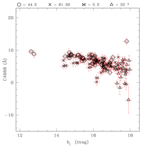
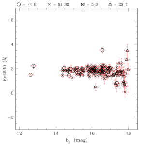
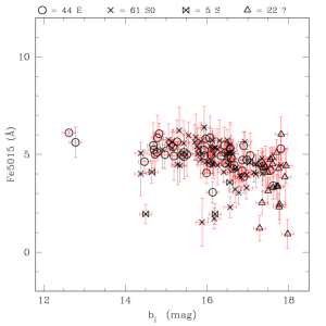
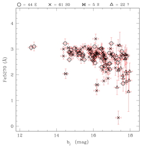
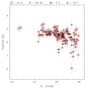
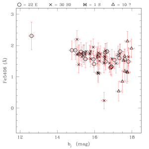
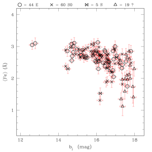
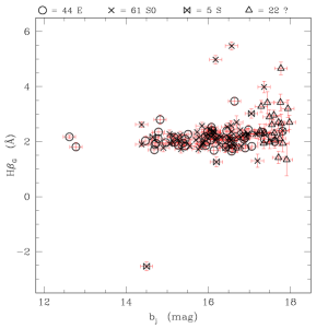
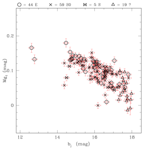
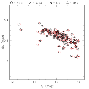
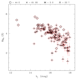
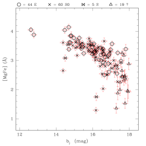
Figure 18: Lick/IDS index absorption line strength data versus magnitude, $b_{j}$. The key at the top of each plot gives the number of ellipticals, lenticulars, spiral bulges and unknown morphological type galaxies. The Mg₁ line strengths have been corrected to the Lick/IDS system by subtracting a mean offset of 0.0204 $\pm$ 0.0025 mag. The Fe5406 line strength errors have been multiplied by 1.647 to correct for an underestimation of the errors demonstrated in the scale test analysis.

Table 16: Lick/IDS index absorption line strength data.

name	C4668	Fe4930	Fe5015	Fe5270	Fe5335	Fe5406	$\langle$Fe$\rangle$	H$\beta$	H$\beta_{\rm{G}}$	Mg1	Mg2	Mgb	$[$MgFe$]$	$[$Oiii$]$sm
d26	0.18	1.38	1.72	1.39	1.22	1.14	1.31	5.16	4.98	0.000	0.088	1.27	1.29	0.00
	0.83	0.15	0.56	0.15	0.20	0.25	0.12	0.13	0.13	0.009	0.006	0.12	0.09	0.10
	41.0	47.3	50.3	53.5	53.3	51.4	53.4	44.0	43.9	52.0	52.0	52.0	52.7	46.5
d27	5.60	1.74	5.08	3.02	2.67		2.84	2.15	2.28	0.092	0.228	3.58	3.19	–0.18
	0.81	0.23	0.51	0.19	0.24		0.15	0.18	0.16	0.008	0.008	0.17	0.11	0.15
	28.2	35.4	37.0	41.3	41.8		41.5	33.3	33.3	38.2	38.1	38.1	39.8	33.8
d28	4.55	1.79	4.55	2.66	2.51	1.76	2.58	1.86	2.06	0.104	0.235	3.91	3.18	–0.17
	0.84	0.15	0.61	0.14	0.18	0.23	0.11	0.12	0.12	0.009	0.006	0.11	0.08	0.13
	41.1	51.4	53.5	60.5	61.7	60.7	61.1	48.3	48.3	55.6	55.8	55.8	58.4	47.7
d29	11.72	1.60	4.99	2.36	2.40	1.49	2.38	1.60	2.03	0.080	0.198	3.68	2.96	–0.55
	0.84	0.26	0.53	0.22	0.25	0.26	0.17	0.20	0.18	0.008	0.008	0.19	0.13	0.76
	24.8	31.7	33.0	36.4	36.7	43.5	36.5	30.1	30.1	34.4	34.3	34.3	35.4	25.8
d38	1.57	0.57	2.03	1.52	1.51	1.11	1.52	0.20	0.68	0.062	0.142	1.93	1.71	–0.85
	0.81	0.24	0.51	0.20	0.23	0.26	0.15	0.19	0.17	0.008	0.007	0.16	0.11	0.26
	27.7	33.6	35.6	40.4	41.4	48.8	40.9	31.4	31.4	37.5	38.2	38.3	39.6	30.7
d39	6.86	1.85	5.01	2.86	2.60	1.69	2.73	1.74	2.08	0.116	0.281	4.08	3.34	–0.02
	0.80	0.15	0.89	0.11	0.14	0.13	0.09	0.09	0.10	0.010	0.006	0.11	0.07	0.10
	50.5	63.7	66.7	76.4	78.8	77.5	77.6	59.8	59.8	69.6	69.5	69.5	73.4	66.8
d40	4.75	1.61	4.10	2.73	2.34	1.50	2.54	2.11	2.31	0.091	0.226	3.78	3.09	–0.19
	0.80	0.18	0.50	0.16	0.21	0.26	0.13	0.15	0.14	0.008	0.007	0.13	0.09	0.24
	32.2	40.5	42.7	48.5	49.8	49.1	49.1	37.9	37.9	44.6	44.7	44.8	46.9	37.9
d42	7.07	1.85	5.75	2.82	2.72	1.81	2.77	1.83	2.08	0.124	0.265	4.43	3.50	–0.28
	0.78	0.15	0.98	0.10	0.13	0.13	0.08	0.09	0.09	0.010	0.006	0.11	0.07	0.11
	51.8	68.6	71.3	84.9	87.2	86.2	86.1	63.7	63.6	75.5	76.7	76.8	81.3	66.2
d44	4.01	2.02	2.12	1.85	2.03		1.94	3.23	3.28	0.032	0.122	2.18	2.05	–3.46
	0.83	0.14	0.61	0.14	0.19		0.12	0.12	0.12	0.009	0.006	0.11	0.08	0.31
	42.4	51.6	54.4	57.5	57.6		57.5	48.3	48.3	55.7	55.7	55.7	56.6	46.8
d50	5.13	1.82	3.57	2.76	1.87		2.32	1.63	2.07	0.080	0.224	3.56	2.87	–0.04
	0.82	0.25	0.52	0.20	0.24		0.16	0.20	0.17	0.008	0.008	0.18	0.12	0.17
	26.0	32.1	33.9	38.4	39.1		38.8	30.3	30.3	35.2	35.4	35.4	37.0	31.3
d53	5.83	1.46	4.85	2.54	2.44	1.49	2.49	1.47	1.74	0.095	0.240	4.17	3.22	0.09
	0.74	0.15	0.96	0.10	0.13	0.13	0.08	0.08	0.09	0.010	0.006	0.11	0.07	0.20
	54.1	68.4	70.5	80.3	81.8	82.8	81.0	64.4	64.4	74.1	74.2	74.3	77.6	70.0
d57	6.00	1.98	5.25	2.84	2.51	1.38	2.68	1.83	2.11	0.094	0.245	3.69	3.14	–0.14
	0.36	0.11	0.53	0.09	0.12	0.13	0.08	0.07	0.06	0.006	0.006	0.09	0.06	0.08
	69.6	87.2	90.8	100.3	101.9	106.0	101.1	82.0	81.9	93.8	93.1	93.2	97.1	83.2
d59	5.69	1.87	5.22	2.43	2.59	1.33	2.51	1.63	1.76	0.102	0.234	3.89	3.12	–0.07
	0.83	0.15	0.77	0.12	0.17	0.13	0.10	0.10	0.11	0.010	0.006	0.11	0.08	0.32
	47.5	59.4	61.2	68.2	69.0	75.1	68.6	56.1	56.1	63.4	63.4	63.4	65.9	54.7
d62	3.63	1.84	4.25	2.22	1.45	0.23	1.83	1.90	2.19	0.060	0.197	3.41	2.50	–0.07
	0.82	0.17	0.55	0.15	0.21	0.25	0.13	0.13	0.13	0.009	0.007	0.13	0.09	0.14
	36.6	45.2	47.6	53.3	53.1	57.0	53.2	42.7	42.7	49.6	49.4	49.5	51.3	42.2
d63	6.10	1.87	3.29	2.78	3.00		2.89	2.19	2.28	0.090	0.221	3.73	3.29	–0.03
	0.87	0.29	0.56	0.23	0.26		0.18	0.22	0.19	0.009	0.008	0.21	0.14	0.17
	23.8	29.8	31.2	34.8	35.4		35.1	28.1	28.1	32.2	32.3	32.3	33.7	28.0
d64	3.04	1.50	3.81	2.22	1.89	1.32	2.06	1.79	2.05	0.065	0.216	3.34	2.62	–0.13
	0.81	0.17	0.52	0.16	0.21	0.26	0.13	0.14	0.14	0.008	0.007	0.13	0.09	0.13
	35.5	43.4	45.6	50.7	51.8	50.7	51.3	40.9	40.9	47.6	47.3	47.4	49.3	42.9
d65	6.67	1.89	4.49	2.91	2.54		2.73	1.92	2.22	0.098	0.265	4.07	3.33	–0.17
	0.84	0.15	0.69	0.13	0.17		0.11	0.11	0.11	0.010	0.006	0.11	0.08	0.11
	44.3	55.2	57.6	65.1	66.5		65.8	52.0	51.9	59.9	59.6	59.6	62.6	55.9
d67	4.59	1.52	5.73	2.87	2.40	1.44	2.64	1.47	1.84	0.113	0.254	4.47	3.43	–0.07
	0.82	0.18	0.54	0.16	0.22	0.28	0.13	0.14	0.14	0.010	0.007	0.13	0.09	0.12
	34.8	44.4	45.7	52.3	53.3	52.6	52.8	41.4	41.4	48.0	48.2	48.2	50.5	44.4
d71	4.94	2.10	4.22	2.69	2.05		2.37	2.25	2.28	0.053	0.178	3.38	2.83	–0.13
	0.79	0.19	0.49	0.18	0.22		0.14	0.16	0.15	0.008	0.007	0.14	0.10	0.25
	31.1	38.9	40.4	44.4	45.0		44.7	36.8	36.7	42.3	42.2	42.2	43.5	33.5
d73	4.70	1.82	4.57	2.45	2.20	1.67	2.32	2.04	2.21	0.059	0.180	2.81	2.56	–0.23
	0.81	0.16	0.52	0.15	0.20	0.25	0.13	0.14	0.13	0.008	0.007	0.12	0.09	0.14
	35.8	44.1	46.2	51.6	52.5	51.7	52.0	41.5	41.5	48.4	48.4	48.4	50.2	39.7
d74	4.46	2.42	3.40	1.67	1.83	1.56	1.75	1.76	2.00	0.052	0.172	3.41	2.44	0.29
	1.07	0.40	0.67	0.30	0.31	0.36	0.22	0.30	0.24	0.009	0.010	0.27	0.17	0.20
	18.9	23.7	25.0	27.9	28.4	28.0	28.2	22.4	22.4	26.2	26.3	26.3	27.2	22.4

Table 17: continued

name	C4668	Fe4930	Fe5015	Fe5270	Fe5335	Fe5406	$\langle$Fe$\rangle$	H$\beta$	H$\beta_{\rm{G}}$	Mg1	Mg2	Mgb	$[$MgFe$]$	$[$Oiii$]$sm
d75	7.63	2.38	5.67	2.99	2.31	1.61	2.65	1.57	1.68	0.071	0.201	2.95	2.79	0.08
	0.81	0.16	0.53	0.15	0.20	0.23	0.13	0.13	0.13	0.009	0.007	0.12	0.09	0.17
	36.2	45.0	46.9	52.2	53.3	58.5	52.7	42.9	42.9	49.1	49.1	49.1	50.9	36.5
d81	5.38	1.95	4.98	2.46	2.15		2.30	2.13	2.41	0.120	0.291	4.70	3.29	–0.03
	0.81	0.19	0.52	0.17	0.22		0.14	0.15	0.14	0.009	0.007	0.14	0.10	0.13
	33.1	40.8	42.4	48.7	49.6		49.2	38.2	38.2	44.1	43.8	43.9	46.4	40.4
d83	7.84	2.12	4.02	0.33	3.30		1.82	4.12	3.81			2.83	2.27	–0.28
	0.89	0.31	0.57	0.26	0.29		0.19	0.24	0.20			0.22	0.15	0.18
	22.8	28.2	29.4	31.3	31.1		31.2	26.1	26.1			30.4	30.8	25.4
d84	6.81	2.17	5.33	2.88	2.56	1.77	2.72	1.96	2.13	0.112	0.275	3.97	3.29	–0.06
	0.80	0.20	0.51	0.17	0.22	0.26	0.14	0.16	0.15	0.009	0.007	0.14	0.10	0.13
	31.9	39.7	41.5	46.8	48.0	47.0	47.4	37.4	37.4	43.0	42.8	42.8	45.0	39.3
d85	5.90	1.65	4.18	2.91	2.14		2.53	1.31	1.77	0.063	0.205	3.50	2.98	–0.67
	0.80	0.21	0.50	0.19	0.23		0.15	0.17	0.15	0.008	0.007	0.16	0.11	0.14
	29.6	36.7	38.4	42.4	42.5		42.5	34.5	34.5	39.8	39.5	39.5	41.0	35.1
d87	5.66	1.74	4.74	2.85	2.84		2.85	1.90	2.10	0.057	0.201	3.51	3.16	–0.09
	0.84	0.14	0.68	0.13	0.17		0.11	0.11	0.11	0.010	0.006	0.11	0.08	0.12
	44.3	55.1	57.4	63.3	64.2		63.8	52.1	52.0	60.2	59.8	59.8	61.8	54.4
d90	4.92	2.15	5.63	3.02	2.85	1.58	2.93	1.97	2.19	0.090	0.239	3.74	3.31	0.01
	0.81	0.16	0.52	0.15	0.20	0.25	0.13	0.14	0.13	0.009	0.007	0.13	0.09	0.12
	35.1	44.5	46.2	52.0	53.3	52.5	52.7	41.8	41.8	48.3	48.1	48.1	50.3	44.9
d93	5.68	1.85	4.31	2.69	2.42	1.51	2.56	1.65	1.84	0.091	0.237	4.16	3.26	–0.12
	0.68	0.15	1.00	0.10	0.13	0.13	0.08	0.08	0.09	0.010	0.006	0.11	0.07	0.15
	56.9	70.4	73.3	82.5	84.2	99.1	83.3	66.5	66.5	76.3	76.3	76.3	79.8	64.8
d98	8.40	1.99	5.79	2.96	3.11		3.04	2.26	2.55	0.095	0.259	4.10	3.53	–0.06
	0.73	0.15	0.98	0.10	0.13		0.08	0.08	0.09	0.010	0.006	0.11	0.07	0.12
	54.7	68.5	71.8	81.7	83.4		82.6	64.2	64.2	75.0	74.5	74.5	78.5	63.4
d107	6.29	1.51	4.94	2.71	2.26		2.49	1.76	2.05	0.064	0.207	3.67	3.02	–0.05
	0.81	0.24	0.51	0.20	0.24		0.16	0.18	0.16	0.008	0.008	0.17	0.12	0.14
	27.3	34.2	35.8	39.3	40.1		39.7	32.5	32.4	37.3	37.0	37.0	38.3	32.4
d108	6.06	1.86	4.78	2.76	2.51	1.55	2.63	1.69	1.96	0.101	0.250	4.30	3.36	–0.19
	0.84	0.14	0.75	0.12	0.16	0.15	0.10	0.10	0.11	0.010	0.006	0.11	0.08	0.15
	45.8	58.1	60.5	68.8	70.0	68.6	69.4	54.7	54.6	63.1	63.1	63.1	66.2	55.6
d110	6.67	1.71	5.24	2.69	2.49	1.84	2.59	1.66	1.88	0.087	0.243	4.21	3.30	–0.09
	0.84	0.15	0.65	0.13	0.18	0.15	0.11	0.11	0.12	0.010	0.006	0.11	0.08	0.12
	42.5	53.5	55.6	62.1	63.3	68.5	62.7	50.5	50.4	57.9	57.6	57.6	60.1	49.7
d112	3.71	2.21	4.09	2.38	2.48		2.43	3.34	3.40	0.012	0.133	2.32	2.37	0.26
	0.82	0.15	0.55	0.15	0.20		0.12	0.13	0.13	0.008	0.006	0.12	0.09	0.38
	38.6	47.1	49.6	53.6	54.2		53.9	44.3	44.3	52.0	51.6	51.6	52.8	41.0
d116	7.42	1.85	5.33	2.72	2.80		2.76	1.90	2.26	0.097	0.251	4.14	3.38	–0.22
	0.77	0.15	0.92	0.11	0.14		0.09	0.09	0.10	0.010	0.006	0.11	0.07	0.10
	52.4	65.5	68.3	76.2	77.2		76.7	61.6	61.6	70.8	70.4	70.4	73.5	64.8
d117	4.98	2.12	5.06	2.29	2.37		2.33	2.08	2.40	0.072	0.209	3.86	3.00	–0.31
	0.82	0.26	0.52	0.21	0.25		0.16	0.20	0.17	0.008	0.008	0.18	0.12	0.15
	26.2	32.4	34.2	38.2	38.4		38.3	30.4	30.4	35.5	35.5	35.5	36.9	31.0
d123	7.72	2.24	5.04	3.02				2.37	2.53			3.62		–0.09
	0.80	0.17	0.52	0.16				0.14	0.14			0.13		0.13
	33.9	42.7	44.8	50.0				40.0	40.0			46.5		41.2
d132	7.60	1.86	5.03	2.62	2.92		2.77	1.56	1.87	0.112	0.288	4.85	3.66	0.02
	0.80	0.18	0.51	0.17	0.22		0.14	0.15	0.14	0.008	0.007	0.14	0.10	0.14
	33.1	41.0	42.3	46.7	47.4		47.1	38.9	38.9	43.5	42.9	42.9	44.9	38.8
d134	5.71	0.82	4.39	2.60	2.25	1.81	2.43	1.74	1.92	0.094	0.262	4.39	3.26	–0.28
	0.84	0.15	0.68	0.13	0.18	0.21	0.11	0.11	0.11	0.010	0.006	0.11	0.08	0.12
	43.4	54.3	56.6	63.7	64.9	63.2	64.3	51.5	51.5	58.9	58.5	58.5	61.3	55.3
d135	6.92	2.02	4.72	3.22	2.78		3.00	1.41	2.19	0.050	0.221	3.78	3.37	–0.39
	0.83	0.26	0.53	0.22	0.26		0.17	0.20	0.17	0.008	0.008	0.19	0.13	0.17
	25.8	32.2	33.9	36.8	37.4		37.1	30.4	30.4	35.3	34.6	34.6	35.8	30.3
d136	7.06	3.52	5.33	2.60	2.48	1.78	2.54	1.48	1.65	0.097	0.263	4.51	3.39	–0.08
	0.72	0.16	1.01	0.10	0.14	0.15	0.09	0.08	0.09	0.010	0.006	0.11	0.07	0.10
	55.3	69.3	72.2	82.0	83.8	82.0	82.9	65.7	65.7	75.3	75.0	75.1	78.9	71.9
d142	7.77	2.02	4.95	2.80	2.62	1.54	2.71	1.58	1.83	0.129	0.301	4.70	3.57	–0.06
	0.76	0.16	0.97	0.11	0.14	0.13	0.09	0.09	0.09	0.011	0.006	0.11	0.07	0.09
	53.2	66.9	69.5	79.0	80.6	78.3	79.8	63.3	63.2	71.8	71.5	71.5	75.5	68.6

Table 18: continued

name	C4668	Fe4930	Fe5015	Fe5270	Fe5335	Fe5406	$\langle$Fe$\rangle$	H$\beta$	H$\beta_{\rm{G}}$	Mg1	Mg2	Mgb	$[$MgFe$]$	$[$Oiii$]$sm
d147	7.22	1.91	5.35	2.81	2.62		2.72	1.97	2.06	0.072	0.230	3.56	3.11	0.17
	0.84	0.15	0.60	0.14	0.19		0.12	0.12	0.12	0.009	0.006	0.12	0.08	0.12
	40.5	50.5	52.8	59.0	59.9		59.4	47.6	47.6	55.1	54.6	54.6	57.0	50.2
d153	6.81	1.68	3.06	2.81	2.26		2.54	1.39	1.51	0.126	0.290	4.16	3.25	–0.29
	0.81	0.17	0.53	0.16	0.21		0.13	0.14	0.13	0.009	0.007	0.13	0.09	0.13
	34.8	44.0	45.9	52.7	54.1		53.4	41.7	41.7	47.7	47.7	47.8	50.5	44.2
d154	3.03	1.70	4.09	2.62	2.30		2.46	1.14	1.59	0.076	0.233	3.18	2.80	–0.29
	0.80	0.17	0.51	0.16	0.20		0.13	0.14	0.14	0.008	0.007	0.13	0.09	0.12
	33.5	42.2	44.7	51.1	52.1		51.6	39.7	39.6	46.9	46.9	46.9	49.2	42.6
d156	5.53	1.83	4.18	2.23	2.41		2.32	1.91	2.07	0.084	0.229	3.80	2.97	–0.10
	0.83	0.15	0.55	0.15	0.20		0.12	0.12	0.13	0.009	0.007	0.12	0.09	0.13
	39.1	47.3	49.0	54.1	55.0		54.5	45.2	45.2	50.8	50.6	50.6	52.5	41.2
d157	6.23	1.64	5.27	3.02	2.46	1.64	2.74	1.84	2.03	0.109	0.269	4.26	3.42	–0.30
	0.78	0.15	0.90	0.11	0.15	0.13	0.09	0.09	0.10	0.010	0.006	0.11	0.07	0.10
	51.6	65.0	67.0	74.8	77.0	75.5	75.9	61.8	61.7	69.7	69.2	69.2	72.5	66.2
d158	4.93	1.39	4.00	2.27	2.61		2.44	1.06	1.30	0.053	0.179	2.77	2.60	0.06
	0.99	0.37	0.64	0.29	0.31		0.21	0.27	0.22	0.009	0.010	0.26	0.17	0.20
	20.3	25.2	26.4	28.9	29.2		29.0	24.0	24.0	27.4	27.2	27.2	28.1	23.0
d161	8.48	1.82	4.96	2.82	2.59		2.71	1.53	1.83	0.123	0.297	4.83	3.62	–0.16
	0.57	0.16	0.98	0.09	0.13		0.08	0.07	0.08	0.009	0.006	0.11	0.07	0.10
	61.4	78.1	80.7	90.1	91.7		90.9	73.9	73.8	83.2	82.3	82.3	86.5	72.8
d171	7.39	2.19	5.50	2.81	2.62	1.64	2.72	1.91	2.22	0.096	0.270	4.17	3.37	–0.23
	0.75	0.15	0.97	0.10	0.13	0.13	0.08	0.09	0.09	0.010	0.006	0.11	0.07	0.09
	53.7	67.8	71.0	81.0	83.2	81.4	82.1	64.0	64.0	74.4	73.9	74.0	77.9	70.7
d181	5.91	2.06	5.05	2.92	2.62	1.66	2.77	1.84	2.06	0.086	0.247	3.81	3.25	–0.13
	0.84	0.15	0.71	0.13	0.17	0.13	0.11	0.10	0.11	0.010	0.006	0.11	0.08	0.16
	45.5	56.5	58.4	64.7	66.4	74.7	65.5	53.7	53.7	60.8	60.2	60.2	62.8	53.0
d182	5.86	1.32	3.84	2.19	2.20		2.20	1.65	1.99	0.111	0.256	4.34	3.09	–0.39
	0.80	0.21	0.51	0.18	0.23		0.15	0.17	0.15	0.009	0.008	0.15	0.11	0.15
	29.4	37.3	39.1	44.0	44.9		44.5	35.2	35.1	40.4	40.4	40.5	42.4	36.4
d191	3.97	2.19	4.27	2.62	2.29		2.45	1.88	2.05	0.096	0.228	3.57	2.96	–0.18
	0.80	0.20	0.50	0.18	0.22		0.14	0.17	0.15	0.008	0.007	0.15	0.10	0.13
	30.4	37.7	39.5	44.5	45.5		45.0	35.5	35.5	41.1	41.2	41.2	43.1	36.6
d192	6.70	2.24	4.43	2.70	2.24	1.67	2.47	2.03	2.18	0.079	0.234	3.55	2.96	0.11
	0.83	0.15	0.59	0.14	0.18	0.13	0.11	0.12	0.12	0.009	0.006	0.11	0.08	0.30
	40.7	50.1	52.6	60.2	62.2	73.8	61.2	47.5	47.5	55.4	55.6	55.6	58.3	45.0
d193	6.62	1.75	5.47	3.03	2.73		2.88	1.57	1.80	0.108	0.268	4.09	3.43	–0.06
	0.80	0.15	0.86	0.11	0.15		0.09	0.09	0.10	0.010	0.006	0.11	0.07	0.09
	50.2	63.0	65.3	72.5	76.1		74.3	59.8	59.8	69.3	68.7	67.0	70.6	62.2
d200	8.17	1.95	5.38	2.75	2.86		2.81	1.87	2.10	0.116	0.287	4.36	3.50	–0.13
	0.26	0.07	0.25	0.09	0.17		0.10	0.07	0.06	0.005	0.007	0.07	0.06	0.10
	74.6	94.0	96.9	107.2	116.6		111.9	89.2	89.2	106.5	104.9	98.7	105.1	87.6
d201	5.60	1.75	4.78	3.15	2.38	1.74	2.77	2.18	2.30	0.055	0.195	2.89	2.83	–0.05
	0.83	0.26	0.52	0.22	0.25	0.28	0.17	0.20	0.17	0.008	0.008	0.19	0.12	0.17
	25.7	31.9	33.3	36.5	37.2	36.7	36.9	30.3	30.3	34.7	34.4	34.4	35.6	30.1
d204	7.39	1.83	4.05	2.56	2.46		2.51	2.00	2.22	0.109	0.244	4.11	3.21	–0.23
	0.82	0.17	0.54	0.16	0.21		0.13	0.14	0.13	0.009	0.007	0.13	0.09	0.13
	35.9	45.0	47.0	53.0	54.1		53.6	42.1	42.1	48.7	48.9	49.0	51.2	44.3
d207	6.32	2.09	5.85	3.10	3.17		3.13	1.79	1.96	0.100	0.255	4.07	3.57	–0.17
	0.76	0.15	0.96	0.11	0.14		0.09	0.09	0.09	0.010	0.006	0.11	0.07	0.09
	53.0	66.9	69.5	78.1	79.9		79.0	63.1	63.1	72.4	72.1	72.1	75.5	67.6
d209	6.00	2.03	4.57	2.68	2.99		2.84	2.14	2.25	0.082	0.229	3.61	3.20	–0.30
	0.80	0.17	0.51	0.16	0.21		0.13	0.14	0.14	0.008	0.007	0.13	0.09	0.13
	34.1	42.4	44.3	48.5	49.4		49.0	40.3	40.3	45.8	45.3	45.3	47.1	41.1
d210	4.37	2.29	5.35	2.78	2.87	1.41	2.83	1.62	1.88	0.119	0.277	4.20	3.44	–0.17
	0.85	0.15	0.77	0.12	0.16	0.13	0.10	0.10	0.11	0.011	0.006	0.11	0.08	0.23
	44.2	57.7	60.7	70.8	73.1	86.1	72.0	54.1	54.1	64.0	64.5	64.5	68.1	52.9
d216	4.60	1.72	4.23	2.49	2.20		2.35	2.82	2.83	0.047	0.158	2.84	2.58	0.06
	0.80	0.20	0.50	0.17	0.22		0.14	0.16	0.15	0.008	0.007	0.14	0.10	0.20
	29.7	38.3	40.8	46.0	46.9		46.5	35.8	35.7	42.9	43.4	43.4	44.9	33.6
d224	6.27	1.62	4.50	2.58	2.60		2.59	1.85	2.16	0.088	0.203	3.02	2.80	–0.18
	0.79	0.20	0.49	0.19	0.23		0.15	0.16	0.15	0.008	0.007	0.15	0.11	0.14
	30.7	37.4	38.7	42.2	42.9		42.5	35.8	35.8	40.0	39.8	39.8	41.1	35.4

Table 19: continued

name	C4668	Fe4930	Fe5015	Fe5270	Fe5335	Fe5406	$\langle$Fe$\rangle$	H$\beta$	H$\beta_{\rm{G}}$	Mg1	Mg2	Mgb	$[$MgFe$]$	$[$Oiii$]$sm
d225	3.45	2.06	4.04	1.99	1.88	1.39	1.94	1.67	1.85	0.067	0.204	3.41	2.57	0.23
	0.80	0.23	0.51	0.20	0.24	0.26	0.15	0.18	0.16	0.008	0.007	0.17	0.11	0.21
	28.2	34.9	36.1	39.7	40.7	40.3	40.2	33.2	33.2	37.8	37.6	37.6	38.9	30.9
d231	5.82	2.18	5.05	2.94	2.48	1.58	2.71	1.85	2.05	0.084	0.245	4.06	3.32	–0.13
	0.84	0.15	0.70	0.13	0.18	0.13	0.11	0.11	0.11	0.010	0.006	0.11	0.08	0.13
	42.6	54.9	57.6	65.0	66.4	76.1	65.7	51.5	51.5	60.3	60.0	60.0	62.8	52.0
ic3943	7.18	1.76	5.97	3.11	2.82	1.81	2.97	1.53	1.79	0.128	0.284	4.07	3.47	–0.08
	0.44	0.13	0.73	0.09	0.13	0.15	0.08	0.07	0.07	0.007	0.006	0.10	0.06	0.07
	66.3	84.6	87.0	97.8	100.5	98.2	99.2	80.1	80.0	90.2	89.8	89.8	94.4	87.2
ic3946	7.76	1.61	4.47	2.89	2.58		2.73	1.89	2.07	0.127	0.282	4.52	3.52	–0.07
	0.82	0.16	0.91	0.12	0.17		0.10	0.09	0.10	0.012	0.007	0.12	0.08	0.10
	49.8	63.4	65.4	73.8	75.7		74.8	59.8	59.7	67.7	67.5	67.5	71.0	64.1
ic3947	5.86	1.94	4.93	2.61	2.47	1.56	2.54	1.58	1.86	0.117	0.272	4.38	3.34	–0.03
	0.54	0.14	0.91	0.09	0.12	0.13	0.08	0.07	0.07	0.008	0.006	0.11	0.07	0.07
	62.5	79.6	82.5	93.6	95.5	93.9	94.6	74.8	74.8	85.5	85.4	85.5	89.9	83.4
ic3959	7.92	1.65	5.66	2.84	2.87	1.80	2.85	1.53	1.79	0.139	0.298	4.94	3.75	–0.15
	0.47	0.14	0.81	0.09	0.14	0.15	0.08	0.07	0.07	0.009	0.007	0.10	0.07	0.09
	65.4	83.9	85.9	97.6	99.5	106.0	98.5	78.9	78.9	89.0	88.9	89.0	93.6	80.8
ic3960	8.84	1.78	4.73	2.98	2.56		2.77	1.59	1.76	0.152	0.311	4.85	3.66	–0.24
	0.50	0.14	0.86	0.09	0.12		0.08	0.07	0.07	0.008	0.006	0.11	0.07	0.09
	63.9	82.0	84.1	95.5	98.0		96.7	77.4	77.3	86.8	86.7	86.8	91.6	83.6
ic3963	4.27	1.80	5.44	2.72	2.65	1.73	2.69	1.54	1.74	0.078	0.227	4.03	3.29	–0.09
	0.77	0.15	0.93	0.11	0.14	0.13	0.09	0.09	0.09	0.010	0.006	0.11	0.07	0.13
	52.3	66.3	68.7	77.1	78.5	81.4	77.8	62.7	62.7	72.0	71.8	71.8	74.7	62.1
ic3973	7.32	1.49	6.22	2.99	2.79	1.64	2.89	2.04	2.24	0.116	0.268	4.42	3.57	–0.04
	0.80	0.17	0.99	0.11	0.16	0.15	0.10	0.09	0.10	0.012	0.007	0.12	0.08	0.09
	51.8	65.8	68.0	78.3	80.6	79.6	79.5	61.8	61.7	71.4	71.7	71.7	75.5	67.9
ic3976	7.28	1.51	5.36	2.86	2.84	1.82	2.85	1.44	1.70	0.139	0.298	4.94	3.75	–0.18
	0.37	0.11	0.49	0.10	0.18	0.16	0.10	0.07	0.06	0.008	0.008	0.08	0.07	0.09
	69.7	89.8	92.2	106.2	108.5	112.2	107.3	84.3	84.2	96.1	96.3	96.4	101.7	93.2
ic3998	7.34	1.97	5.63	2.96	2.71		2.83	1.83	2.08	0.108	0.273	4.16	3.43	–0.10
	0.74	0.15	0.97	0.11	0.12		0.08	0.08	0.09	0.008	0.006	0.11	0.07	0.11
	54.1	68.4	70.8	78.1	90.4		84.2	64.3	64.3	83.3	82.4	72.4	78.1	61.9
ic4011	8.29	1.64	4.54	2.69	2.37		2.53	2.17	2.42	0.126	0.273	4.30	3.30	–0.17
	0.81	0.17	0.54	0.16	0.21		0.13	0.14	0.13	0.009	0.007	0.13	0.09	0.13
	35.3	44.3	46.3	52.5	53.6		53.1	41.5	41.5	47.8	48.0	48.0	50.5	44.1
ic4012	8.55	1.90	5.23	2.79	2.80		2.79	1.86	2.09	0.128	0.286	4.55	3.56	–0.14
	0.56	0.15	0.97	0.09	0.13		0.08	0.07	0.08	0.009	0.006	0.11	0.07	0.08
	61.7	78.2	80.8	90.7	92.2		91.4	73.7	73.7	83.2	82.7	82.8	87.0	78.0
ic4026	8.32	2.13	5.88	3.04	3.10	1.75	3.07	2.00	2.28	0.111	0.271	4.13	3.56	–0.11
	0.63	0.15	1.00	0.10	0.12	0.13	0.08	0.08	0.08	0.009	0.006	0.11	0.07	0.08
	59.0	73.7	76.9	86.3	87.9	85.9	87.1	69.4	69.4	79.7	79.2	79.2	83.1	75.8
ic4041	8.06	1.93	6.38	2.92	2.80	1.95	2.86	1.88	2.15	0.108	0.285	4.34	3.52	–0.10
	0.78	0.15	0.90	0.11	0.14	0.13	0.09	0.09	0.10	0.010	0.006	0.11	0.07	0.09
	51.5	64.1	67.1	76.6	78.4	76.8	77.5	60.3	60.3	70.1	69.6	69.6	73.5	66.9
ic4042	8.13	1.52	4.43	2.59	2.69		2.64	1.38	1.63	0.115	0.278	4.47	3.43	–0.16
	0.85	0.16	0.76	0.13	0.18		0.11	0.10	0.11	0.011	0.007	0.12	0.08	0.10
	45.5	57.2	59.6	67.8	69.2		68.5	53.9	53.9	61.8	61.8	61.8	65.0	57.8
ic4045	8.40	2.14	5.39	2.90	2.68	1.73	2.79	1.73	2.00	0.141	0.314	4.77	3.65	–0.24
	0.29	0.09	0.33	0.10	0.18	0.15	0.10	0.07	0.06	0.006	0.007	0.07	0.06	0.09
	73.2	91.5	95.3	109.3	112.4	110.3	110.9	86.6	86.5	98.7	98.4	98.5	104.5	94.5
ic4051	8.07	2.05	4.63	3.22	2.50		2.86	1.45	2.03	0.180	0.371	5.71	4.04	–0.05
	0.83	0.20	0.58	0.16	0.23		0.14	0.14	0.14	0.011	0.008	0.14	0.10	0.14
	33.4	43.8	46.2	56.1	58.0		57.0	40.8	40.8	48.1	48.6	48.7	52.7	45.9
ngc4848	5.08	1.84	2.01	2.08	2.54		2.31	–4.82	–4.39	0.080	0.200	4.05	3.06	–3.26
	0.80	0.18	0.52	0.17	0.21		0.14	0.14	0.14	0.009	0.007	0.14	0.10	0.43
	33.5	41.7	44.1	47.8	51.4		49.6	40.5	40.5	52.1	52.1	45.1	47.3	38.5
ngc4850	6.70	1.88	4.92	2.77	2.57	1.74	2.67	1.28	1.57	0.107	0.264	4.40	3.43	–0.58
	0.45	0.12	0.52	0.09	0.17	0.15	0.10	0.07	0.07	0.006	0.007	0.08	0.06	0.12
	65.9	86.7	91.2	106.2	109.4	107.8	107.8	80.9	80.8	95.9	96.6	96.7	102.1	93.3
ngc4851	7.08	1.65	4.63	2.55	2.68		2.62	1.85	2.02	0.081	0.256	4.10	3.27	–0.38
	0.81	0.17	0.53	0.16	0.22		0.14	0.14	0.13	0.009	0.007	0.13	0.09	0.14
	34.8	43.7	45.6	50.0	50.9		50.5	41.5	41.5	47.2	46.5	46.5	48.5	42.3

Table 20: continued

name	C4668	Fe4930	Fe5015	Fe5270	Fe5335	Fe5406	$\langle$Fe$\rangle$	H$\beta$	H$\beta_{\rm{G}}$	Mg1	Mg2	Mgb	$[$MgFe$]$	$[$Oiii$]$sm
ngc4853	5.09	1.45	4.01	2.73	2.04		2.38	1.98	2.11	0.058	0.160	2.95	2.65	–0.85
	0.54	0.15	0.94	0.09	0.12		0.08	0.07	0.08	0.008	0.006	0.11	0.07	0.08
	62.3	77.4	81.0	88.5	89.5		89.0	72.8	72.7	84.2	84.6	84.7	86.8	78.7
ngc4860	9.27	1.86	5.46	2.89	3.28		3.08	1.33	1.70	0.154	0.342	5.57	4.14	0.21
	0.78	0.19	1.05	0.12	0.18		0.11	0.09	0.10	0.013	0.008	0.13	0.08	0.09
	53.8	67.3	68.6	76.6	77.8		77.2	64.0	64.0	70.3	69.2	69.3	73.1	65.7
ngc4864	7.55	1.74	5.25	2.59	2.53		2.56	1.61	1.82	0.130	0.286	4.47	3.38	–0.12
	0.34	0.10	0.47	0.09	0.14		0.08	0.07	0.06	0.006	0.007	0.09	0.06	0.08
	70.5	89.4	92.2	103.4	105.3		104.3	84.4	84.3	95.0	94.5	94.7	99.4	91.5
ngc4867	7.43	1.45	5.11	2.74	2.57	1.70	2.65	1.61	1.95	0.129	0.297	4.55	3.47	–0.23
	0.26	0.03	0.14	0.10	0.18	0.15	0.10	0.07	0.06	0.006	0.007	0.07	0.06	0.08
	77.8	99.7	102.6	117.3	121.0	119.5	119.1	93.5	93.5	106.9	106.7	106.8	112.8	106.7
ngc4869	8.29	1.85	4.96	2.99	2.84	1.86	2.92	1.52	1.81	0.144	0.311	4.86	3.77	–0.27
	0.36	0.10	0.48	0.09	0.16	0.15	0.09	0.07	0.06	0.007	0.007	0.09	0.06	0.11
	69.8	89.5	92.1	104.8	107.1	111.6	106.0	84.4	84.3	95.1	94.8	94.8	100.2	86.9
ngc4872	8.76	2.00	5.85	2.96	3.05		3.01	1.91	2.13	0.133	0.299	4.90	3.84	–0.37
	0.82	0.17	1.01	0.11	0.15		0.09	0.09	0.10	0.012	0.007	0.12	0.08	0.10
	50.2	66.4	69.3	80.1	81.9		81.0	62.1	62.1	72.2	72.3	72.3	76.5	67.8
ngc4873	6.08	1.53	5.65	2.73	2.58	1.73	2.65	1.70	1.91	0.126	0.300	4.52	3.47	–0.11
	0.47	0.13	0.72	0.09	0.14	0.15	0.08	0.07	0.07	0.007	0.006	0.10	0.06	0.09
	65.2	83.9	87.3	100.8	104.0	102.2	102.4	78.2	78.1	91.4	91.2	91.2	96.7	90.0
ngc4874	8.78	2.24	5.62	3.10	3.10		3.10	1.65	1.81	0.133	0.306	4.86	3.88	–0.04
	0.89	0.19	0.76	0.15	0.23		0.14	0.11	0.12	0.013	0.009	0.13	0.09	0.12
	42.1	54.4	56.5	64.4	65.7		65.0	51.6	51.5	58.4	58.0	58.1	61.5	54.4
ngc4875	7.16	1.74	2.45	2.83	2.63		2.73	1.62	1.87	0.143	0.289	4.62	3.55	–0.05
	0.55	0.15	0.96	0.09	0.13		0.08	0.07	0.08	0.009	0.006	0.11	0.07	0.09
	62.2	78.7	81.4	92.1	94.1		93.1	74.0	73.9	83.7	84.2	84.2	88.5	73.4
ngc4876	6.83	1.88	5.15	2.60	2.70	1.62	2.65	1.92	2.18	0.097	0.262	3.95	3.24	–0.16
	0.65	0.16	1.02	0.10	0.13	0.13	0.08	0.08	0.09	0.010	0.006	0.11	0.07	0.12
	58.4	72.3	76.0	86.5	89.0	93.4	87.8	68.2	68.2	79.7	79.2	79.3	83.4	67.8
ngc4881	8.30	1.43	5.02	2.86	2.54		2.70	1.67	1.94	0.132	0.291	4.85	3.62	–0.06
	0.58	0.15	0.94	0.09	0.13		0.08	0.07	0.08	0.009	0.006	0.11	0.07	0.08
	61.0	79.1	82.3	94.7	96.3		95.5	74.4	74.3	85.4	85.6	85.7	90.5	80.5
ngc4883	6.99	2.03	5.67	3.06	2.77		2.91	1.63	1.97	0.115	0.289	4.39	3.58	–0.07
	0.61	0.15	1.00	0.09	0.12		0.08	0.08	0.08	0.009	0.006	0.11	0.07	0.10
	59.8	76.2	79.1	89.2	91.0		90.1	71.8	71.8	82.1	81.2	81.2	85.5	70.1
ngc4886	8.49	2.01	6.06	2.85	3.36		3.11	2.49	2.80	0.144	0.290	4.76	3.85	–0.04
	0.83	0.25	0.53	0.20	0.25		0.16	0.19	0.17	0.009	0.008	0.17	0.12	0.16
	26.8	35.0	36.3	41.7	42.6		42.1	32.4	32.4	37.4	37.4	37.4	39.7	33.9
ngc4889	9.59	1.49	6.10	3.06	3.03	2.31	3.05	1.86	2.03	0.166	0.361	5.39	4.05	–0.26
	0.29	0.04	0.17	0.12	0.27	0.23	0.15	0.07	0.06	0.010	0.011	0.08	0.08	0.07
	91.6	117.8	122.0	141.6	146.0	143.1	143.8	110.7	110.7	126.3	125.6	125.7	134.4	127.2
ngc4894	4.76	1.33	5.02	3.03	3.18		3.11	1.25	1.97	0.076	0.233	3.51	3.30	0.04
	0.80	0.17	0.53	0.15	0.19		0.12	0.14	0.14	0.009	0.007	0.12	0.09	0.13
	33.4	43.5	46.5	55.0	56.8		55.9	40.7	40.6	49.5	49.9	49.9	52.8	45.9
ngc4895	6.76	1.83	4.96	3.11	2.74		2.93	1.48	1.78	0.122	0.286	4.54	3.65	–0.18
	0.26	0.06	0.17	0.10	0.19		0.11	0.07	0.06	0.006	0.008	0.07	0.06	0.12
	75.2	95.7	99.4	111.2	113.4		112.3	90.3	90.3	114.6	113.7	102.0	107.0	89.6
ngc4896	6.38	1.96	5.68	2.87	2.56	1.62	2.71	1.94	2.24	0.129	0.303	4.26	3.40	–0.20
	0.84	0.15	0.77	0.12	0.17	0.13	0.11	0.10	0.11	0.011	0.007	0.11	0.08	0.24
	46.2	58.1	60.3	69.1	71.2	70.5	70.1	54.7	54.7	63.0	62.6	62.7	66.3	57.6
ngc4906	7.63	1.96	4.85	2.78	2.60	1.75	2.69	1.55	1.85	0.134	0.306	4.66	3.54	–0.07
	0.56	0.15	0.97	0.09	0.12	0.15	0.08	0.07	0.08	0.009	0.006	0.11	0.07	0.10
	61.7	77.4	80.6	91.9	94.0	97.6	93.0	73.2	73.2	83.4	83.0	83.1	87.9	79.5
ngc4907	8.16	1.86	4.10	3.05	2.90		2.97	1.12	1.55	0.113	0.268	4.21	3.54	–1.03
	0.83	0.17	0.58	0.15	0.20		0.13	0.13	0.13	0.010	0.007	0.12	0.09	0.12
	36.6	47.1	49.7	56.8	58.2		57.5	44.3	44.2	51.4	51.5	51.6	54.4	47.3
ngc4908	5.98	1.25	5.24	2.77	2.76		2.76	1.18	1.44	0.121	0.265	4.46	3.51	–0.56
	0.83	0.16	0.89	0.12	0.17		0.10	0.10	0.10	0.012	0.007	0.12	0.08	0.10
	48.9	62.2	64.7	72.5	73.7		73.1	58.5	58.5	66.8	66.7	66.8	69.9	61.7
ngc4919	7.96	1.77	5.49	3.04	2.79	2.20	2.92	1.61	1.92	0.123	0.308	4.49	3.62	0.08
	0.26	0.03	0.14	0.10	0.17	0.15	0.10	0.07	0.06	0.005	0.007	0.07	0.06	0.09
	81.6	101.8	106.3	121.0	124.1	120.4	122.6	95.9	95.7	110.4	109.3	109.3	115.8	108.0

Table 21: continued

name	C4668	Fe4930	Fe5015	Fe5270	Fe5335	Fe5406	$\langle$Fe$\rangle$	H$\beta$	H$\beta_{\rm{G}}$	Mg1	Mg2	Mgb	$[$MgFe$]$	$[$Oiii$]$sm
ngc4923	8.56	1.77	5.13	2.79	2.84	1.85	2.82	1.78	2.11	0.135	0.303	4.62	3.61	–0.04
	0.31	0.09	0.35	0.10	0.18	0.15	0.10	0.07	0.06	0.006	0.007	0.07	0.06	0.09
	72.2	90.9	94.5	109.5	112.8	117.9	111.2	85.8	85.7	98.5	98.6	98.7	104.7	95.5
rb58	5.53	0.55	6.02	2.03				1.35	1.94			3.85		0.36
	1.36	0.51	0.83	0.40				0.38	0.30			0.35		0.27
	15.7	19.6	20.7	22.6				18.5	18.5			21.4		17.3
rb60	3.00	1.89	4.50	2.79	2.78	1.52	2.79	2.34	2.44	0.072	0.207	3.13	2.95	–0.05
	0.83	0.27	0.53	0.22	0.25	0.26	0.17	0.21	0.18	0.008	0.008	0.19	0.13	0.20
	25.3	31.3	32.9	36.4	36.9	39.8	36.6	29.5	29.5	34.0	33.9	33.9	35.3	26.7
rb66	–0.30	1.73	3.36	2.61	1.63		2.12	0.96	1.42	0.013	0.143	2.54	2.32	0.50
	0.95	0.36	0.61	0.26	0.28		0.19	0.27	0.22	0.008	0.009	0.24	0.15	0.19
	21.1	25.4	27.5	30.8	31.3		31.0	24.0	24.0	28.8	28.9	29.0	30.0	24.6
rb74	5.58	1.45	3.04	2.27	2.11		2.19	1.95	2.23	0.052	0.169	2.86	2.50	–0.31
	0.92	0.34	0.59	0.25	0.27		0.19	0.25	0.21	0.008	0.009	0.22	0.15	0.17
	21.9	26.9	28.6	32.2	32.9		32.6	25.4	25.4	30.1	30.2	30.2	31.4	25.9
rb94	4.42	1.18	3.22	2.11	2.63		2.37	2.73	2.70	0.052	0.188	3.30	2.80	–0.11
	1.04	0.40	0.67	0.29	0.31		0.21	0.30	0.24	0.009	0.010	0.27	0.17	0.20
	19.3	23.7	25.3	28.7	29.1		28.9	22.2	22.2	26.6	26.7	26.7	27.8	22.5
rb122	4.29	1.48	3.31	1.86	2.05	1.17	1.96	1.57	2.05	0.042	0.204	3.06	2.44	–0.16
	0.90	0.32	0.58	0.24	0.27	0.30	0.18	0.24	0.20	0.009	0.009	0.22	0.14	0.17
	22.5	27.8	29.5	33.4	33.6	33.0	33.5	26.3	26.3	30.9	30.6	30.6	32.0	26.8
rb128	4.22	1.58	2.53	2.16	1.77		1.96	1.49	1.81	0.099	0.218	3.80	2.73	–0.23
	0.87	0.31	0.57	0.23	0.27		0.18	0.22	0.19	0.010	0.009	0.20	0.14	0.18
	24.1	29.9	31.7	36.0	36.7		36.4	28.3	28.3	32.8	33.2	33.2	34.8	28.9
rb129	5.27	1.72	4.15	2.41	2.08	1.29	2.24	1.82	2.05	0.097	0.254	3.73	2.89	–0.24
	0.83	0.15	0.58	0.14	0.19	0.20	0.12	0.12	0.12	0.009	0.006	0.12	0.08	0.12
	40.3	49.5	51.7	58.8	60.2	63.5	59.5	46.8	46.8	54.0	53.8	53.8	56.6	49.2
rb131	–0.49	0.67	2.45	1.72				3.00	2.65			2.17		–0.01
	1.36	0.55	0.89	0.46				0.42	0.33			0.38		0.29
	15.7	18.3	19.5	20.5				17.1	17.1			20.3		15.9
rb153	6.80	3.47	4.42	1.78	1.05		1.42	2.93	2.57	0.017	0.116	2.63	1.93	–1.05
	1.63	0.54	0.85	0.39	0.39		0.28	0.42	0.32	0.011	0.012	0.35	0.22	0.27
	14.0	18.7	20.4	22.9	23.2		23.1	17.3	17.3	21.5	21.8	21.8	22.4	17.2
rb198	4.35	0.55	4.09	2.51	2.11	1.65	2.31	1.77	2.10	0.071	0.174	2.52	2.41	–0.28
	0.90	0.31	0.58	0.25	0.27	0.31	0.19	0.24	0.20	0.008	0.009	0.22	0.14	0.21
	22.4	28.0	29.3	32.3	32.8	32.1	32.5	26.5	26.4	30.5	30.7	30.7	31.6	24.2
rb223	6.22	1.66	4.51	2.75	2.55	1.66	2.65	2.04	2.14	0.096	0.235	3.99	3.25	–0.28
	0.84	0.14	0.68	0.13	0.17	0.20	0.11	0.11	0.11	0.010	0.006	0.11	0.08	0.10
	43.7	55.0	57.3	64.0	65.2	63.9	64.6	51.8	51.8	59.3	59.4	59.5	62.0	56.0
rb245	2.54	0.94	3.36	2.62	2.58	1.17	2.60	1.77	2.12	0.027	0.146	2.28	2.43	0.39
	1.38	0.49	0.77	0.34	0.35	0.40	0.24	0.37	0.29	0.010	0.011	0.31	0.20	0.23
	15.6	20.4	22.0	25.1	25.8	25.5	25.5	19.0	19.0	23.6	23.7	23.7	24.6	19.7
gmp1986	–5.33	2.73	3.85	1.34	2.13		1.74	1.90	1.34	-0.008	0.045	2.21	1.96	–0.17
	3.29	0.83	1.49	0.81	0.78		0.56	0.76	0.57	0.021	0.021	0.60	0.41	0.54
	9.1	10.9	11.9	13.3	13.3		13.3	10.3	10.3	12.6	12.8	12.8	13.1	9.6
gmp2421	2.11	1.91	1.75	2.11	2.75	1.91	2.43	1.73	2.26	0.052	0.203	3.16	2.77	0.59
	1.09	0.40	0.64	0.28	0.29	0.30	0.20	0.31	0.24	0.009	0.009	0.26	0.16	0.50
	18.5	23.6	25.8	29.3	30.4	32.3	29.9	22.0	22.0	27.1	27.1	27.1	28.5	20.6
gmp2688	7.06	1.82	5.10	2.80	2.89		2.85	2.41	2.70	0.064	0.174	3.53	3.17	0.22
	0.96	0.36	0.62	0.27	0.30		0.20	0.27	0.22	0.009	0.009	0.25	0.16	0.18
	20.9	25.5	27.0	30.1	30.2		30.1	23.9	23.9	28.1	28.2	28.3	29.2	23.8
gmp2721	1.65	1.78	3.13	2.68	1.29		1.98	2.32	1.98	0.080	0.185	2.55	2.25	0.00
	1.06	0.40	0.66	0.29	0.30		0.21	0.30	0.24	0.009	0.010	0.26	0.17	0.20
	19.0	24.0	25.5	28.7	29.2		29.0	22.5	22.4	26.5	26.9	26.9	27.9	22.7
gmp2783	2.79	0.62	4.31	2.20	0.04		1.12	1.65	2.05	0.029	0.123	3.14	1.88	–0.46
	1.48	0.53	0.88	0.40	0.42		0.29	0.41	0.31	0.011	0.012	0.37	0.23	0.27
	14.9	18.8	19.6	22.6	21.9		22.2	17.7	17.7	20.6	20.8	20.8	21.5	17.0
gmp2942	5.41	1.67	4.27	2.40	2.08		2.24	1.49	1.77	0.101	0.257	4.51	3.18	–0.07
	0.81	0.20	0.52	0.18	0.23		0.15	0.15	0.15	0.009	0.008	0.14	0.10	0.13
	32.4	40.1	42.1	47.1	47.6		47.4	37.8	37.8	43.4	43.3	43.3	45.3	39.3
gmp3012	4.32	2.44	4.08	2.26	0.91	0.85	1.59	2.26	2.60	0.038	0.186	2.49	1.99	–0.49
	1.07	0.44	0.72	0.33	0.34	0.41	0.24	0.31	0.25	0.010	0.011	0.30	0.19	0.23
	18.9	22.4	23.7	25.8	26.3	24.9	26.1	21.6	21.5	24.7	24.4	24.4	25.2	20.7

Table 22: continued

name	C4668	Fe4930	Fe5015	Fe5270	Fe5335	Fe5406	$\langle$Fe$\rangle$	H$\beta$	H$\beta_{\rm{G}}$	Mg1	Mg2	Mgb	$[$MgFe$]$	$[$Oiii$]$sm
gmp3298	4.15	1.58	4.69	2.61	2.38	1.69	2.50	2.13	2.35	0.048	0.180	3.16	2.81	–0.34
	0.99	0.37	0.64	0.28	0.30	0.30	0.20	0.28	0.23	0.009	0.009	0.25	0.16	0.40
	20.2	25.1	26.3	29.4	30.0	33.2	29.7	23.5	23.5	27.8	27.8	27.8	28.7	21.9
gmp3585	–0.23	0.79	1.17	1.51	1.18	0.54	1.34	2.07	2.31	0.016	0.048	1.37	1.36	–1.63
	0.91	0.36	0.61	0.28	0.30	0.35	0.21	0.27	0.22	0.009	0.009	0.24	0.16	0.21
	22.0	25.7	27.3	29.5	29.7	29.1	29.6	24.1	24.1	28.4	29.1	29.0	29.3	24.4
gmp3588	2.66	1.12	4.26	2.92	1.89	2.13	2.40	3.28	3.19	0.022	0.138	2.42	2.41	–0.32
	1.11	0.45	0.75	0.35	0.35	0.33	0.25	0.33	0.26	0.010	0.011	0.30	0.20	0.30
	18.3	22.0	22.8	25.1	25.7	29.7	25.4	20.7	20.7	24.1	24.1	24.1	24.8	18.4
gmp3829	–1.58	1.42	4.35	3.15				3.07	3.05			3.26		–0.61
	1.69	0.61	1.00	0.52				0.47	0.36			0.45		0.33
	13.7	16.5	17.6	18.6				15.8	15.8			17.6		14.1
gmp4348	3.04	0.76	2.35	2.02	1.82	1.14	1.92	4.92	4.59	–0.014	0.041	1.21	1.52	0.14
	0.92	0.35	0.61	0.28	0.30	0.33	0.21	0.27	0.22	0.009	0.009	0.24	0.16	0.22
	21.8	25.9	27.4	29.4	29.3	30.4	29.4	23.9	23.9	28.7	29.0	29.0	29.2	23.6
gmp4420	5.26	1.63	4.94	2.00	2.21		2.11	2.31	2.74	0.048	0.179	3.05	2.54	0.21
	0.80	0.19	0.49	0.18	0.20		0.13	0.15	0.14	0.008	0.006	0.14	0.10	0.29
	32.5	39.6	41.4	44.5	53.9		49.2	37.5	37.5	51.5	51.0	42.7	45.8	30.3

Notes: There are three lines for each galaxy in this table. The first line gives the absorption line strength data, whilst errors are given on the second line and signal-to-noise values for each index are given on the third. Missing values in the table indicate either that the line strength measured had a low S/N or that it could not be measured. The H$\beta$ and H$\beta_{\rm{G}}$ line strengths given in the table have not been corrected for nebula emission. The Mg₁ line strengths have been corrected to the Lick/IDS system by subtracting a mean offset of 0.0204 $\pm$ 0.0025 mag. The Fe5406 line strength errors have been multiplied by 1.647 to correct for an underestimation of the errors demonstrated in the scale test analysis. There are a total of 132 galaxies in this data table.

References

- [1] Aragón-Salamanca A., Ellis R. S., Couch W. J., Carter D., 1993, MNRAS, 262, 764
- [2] Baugh C. M., Cole S., Frenk C. S., 1996, MNRAS, 283, 1361
- [3] Bender R., Burstein D., Faber S. M., 1992, ApJ, 399, 462
- [4] Bender R., Burstein D., Faber S. M., 1993, ApJ, 411, 153
- [5] Bernardi M., Renzini A., da Costa L. N., Wegner G., Alonso M. V., Pellegrini P.S., Rité C., Willmer C. N. A., 1998, ApJ, 508, 143
- [6] Binggeli B., Sandage A., Tammann G. A., 1988, ARA&A, 26, 509
- [7] Biviano A., Durret F., Gerbal D., Le Fevre O., Lobo C., Mazure A., Slezak E., 1995, A&A, 297, 610
- [8] Bower R. G., Lucey J. R., Ellis R. S., 1992, MNRAS, 254, 601
- [9] Burstein D., 1979, ApJ, 234, 435
- [10] Burstein D., Faber S. M., Gaskell C. M., Krumm N., 1984, ApJ, 287, 586
- [11] Burstein D., Davies R. L., Dressler A., Faber S. M., Lynden-Bell D., 1988, in Proc. of the Fifth Workshop of the Advanced School of Astronomy, Towards Understanding Galaxies At Large Redshift. Kluwer, Dordrecht, p. 17
- [12] Caldwell N., 1984, PASP, 96, 287
- [13] Caldwell N., Rose J. A., 1997, AJ, 113, 492
- [14] Caldwell N., Rose J. A., Sharples R. M., Ellis R. S., Bower R. G., 1993, AJ, 106, 473
- [15] Castander F. J. et al., 2001, AJ, 121, 2331
- [16] Ciotti L., Lanzoni B., Renzini A., 1996, MNRAS, 282, 1
- [17] Colless M., Burstein D., Davies R. L., McMahan R. K., Saglia R. P., Wegner G., 1999, MNRAS, 303, 813
- [18] Cowie L. L., Songaila A., 1977, Nature, 266, 501
- [19] Djorgovski S., Davis M., 1987, ApJ, 313, 59
- [20] van Dokkum P. G., Franx M, 1995, AJ, 110, 2027
- [21] van Dokkum P. G., Franx M, Kelson D. D., Illingworth G. D., Fisher D., Fabricant D., 1998, ApJ, 500, 714
- [22] Dressler A., 1980a, ApJS, 42, 565
- [23] Dressler A., 1980b, ApJ, 236, 351
- [24] Dressler A., Lynden-Bell D., Burstein D., Davies R. L., Faber S. M., Terlevich R., Wegner G., 1987, ApJ, 313, 42
- [25] Dressler A., Oemler A., Couch W. J., Smail I., Ellis R. S., Barger A., Butcher H., Poggianti B. M., Sharples R. M., 1997, ApJ, 490, 577
- [26] Dreyer J. L. E., 1888, ‘A New General Catalogue of Nebulae and Clusters of Stars, being the Catalogue of the late Sir John F.W. Herschel, Bart., revised, corrected, and enlarged’, Mem. R. Astron. Soc., 49, 1
- [27] Dreyer J. L. E., 1908, ‘Index Catalogue of Nebulae and Clusters of Stars (IC 1530–5386), containing objects found in the years 1895 to 1907; with Notes and Corrections to the New General Catalogue and to the Index Catalogue for 1888-94’, Mem. R. Astron. Soc., 59, 105
- [28] Ellis R. S., Smail I., Dressler A., Couch W. J., Oemler A., Butcher H., Sharples R. M., 1997, ApJ, 483, 582
- [29] Edwards S. A., Colless M., Bridges T. J., Carter D., Mobasher B., Poggianti B. M., 2002, ApJ, in press (astro-ph/0111038)
- [30] Faber S. M., 1973, ApJ, 179, 731
- [31] Faber S. M., Gallagher J. S., 1976, ApJ, 204, 365
- [32] Faber S. M., Friel E. D., Burstein D., Gaskell C. M., 1985, ApJS, 57, 711
- [33] Faber S. M., Dressler A., Davies R. L., Burstein D., Lynden-Bell D., 1987, in Proc. of the Eighth Santa Cruz Summer Workshop in Astronomy and Astrophysics, Nearly normal galaxies: From the Planck time to the present. Springer-Verlag, New York, p. 175-183
- [34] Fasano G., Poggianti B. M., Couch W. J., Bettoni D., Kjaergaard P., Moles M., 2000, ApJ, 542, 673
- [35] Godwin J. G., Metcalfe N., Peach J. V., 1983, MNRAS, 202, 113
- [36] González J. J., 1993, PhD thesis, University of California, Santa Cruz
- [37] Goudfrooij P., Emsellem E., 1996, A&A, 306, 45
- [38] Goudfrooij P., Hansen L., Jorgensen H. E., Norgaard-Nielsen H. U., de Jong T., van den Hoek L. B., 1994, A&AS, 104, 179
- [39] Gunn J. E., Gott J. R., 1972, ApJ, 176, 1
- [40] Guzmán R., Lucey J. R., Bower R. G., 1993, MNRAS, 265, 731
- [41] Hambly N. C., Davenhall A. C., Irwin M. J., MacGillivray H. T., 2001, MNRAS, 326, 1315
- [42] Ho L. C., Filippenko A. V., Sargent W. L. W., 1997, ApJS, 112, 315
- [43] Hudson M. J., Lucey J. R., Smith R. J., Schlegel D. J., Davies R. L., 2001, MNRAS, 327, 265
- [44] Jørgensen I., 1997, MNRAS, 288, 161
- [45] Jørgensen I., 1999, MNRAS, 306, 607
- [46] Jørgensen I., Franx M., Kjaergaard P., 1995a, MNRAS, 273, 1097
- [47] Jørgensen I., Franx M., Kjaergaard P., 1995b, MNRAS, 276, 1341
- [48] Kauffmann G., 1996, MNRAS, 281, 487
- [49] Kelson D. D., Illingworth G. D., van Dokkum P. G., Franx M., 2000, ApJ, 531, 184
- [50] Kodama T., Smail I., 2001, MNRAS, 326, 637
- [51] Kodama T., Arimoto N., Barger A., Aragón-Salamanca A., 1998, A&A, 334, 99
- [52] Kuntschner H., 2000, MNRAS, 315, 184
- [53] Kuntschner H., Davies R. L., 1998, MNRAS, 295, 29
- [54] Kuntschner H., Lucey J. R., Smith R. J., Hudson M. J., Davies R. L., 2001, MNRAS, 323, 615
- [55] Larson R. B., 1975, MNRAS, 173, 671
- [56] Larson R. B., Tinsley B. M., Caldwell C. N., 1980, ApJ, 237, 692
- [57] Massey P., Strobel K., Barnes J. V., Anderson E., 1988, ApJ, 328, 315
- [58] Mehlert D., Saglia R. P., Bender R., Wegner G., 2000, A&AS, 141, 449
- [59] Monet D. et al., 1997, USNOA2, ‘A Catalog of Astrometric Standards’, www.nofs.navy.mil/data/fchpix/
- [60] Moore B., Lake G., Katz N., 1998, ApJ, 495, 139
- [61] Moore S. A. W., 2001, PhD thesis, University of Durham, UK
- [62] Moore S. A. W., Lucey J. R., Kuntschner H., Davies R. L., Colless M., 2001, Ap&SS, 277, 429
- [63] Moore S. A. W., Lucey J. R., Kuntschner H., Colless M., 2002a, MNRAS, Paper II, in preparation
- [64] Moore S. A. W., Lucey J. R., Kuntschner H., Colless M., 2002b, MNRAS, Paper III, in preparation
- [65] Phillips M. M., Jenkins C. R., Dopita M. A., Sadler E. M., Binette L., 1986, AJ, 91, 1062
-
[66]
Pollacco D., Bridges T. J., Rees P. C. T., Lewis J. R., Boyle B. J., Lewis I., King D. L., 1999, ‘
AUTOFIB2/WYFFOSUser Manual’, www.ing.iac.es/Astronomy/instruments/af2/af2manual.ps.gz - [67] Poggianti B. M., Smail I., Dressler A., Couch W. J., Barger A. J., Butcher H., Ellis R. S., Oemler A., 1999, ApJ, 518, 576
- [68] Poggianti B. M. et al., 2001, preprint (astro-ph/0108212)
- [69] Rood H. J., Baum W. A., 1967, AJ, 72, 398
- [70] Sargent W. L. W., Schechter P. L., Boksenberg A., Shortridge K., 1977, ApJ, 212, 326
- [71] Spitzer L., Baade W., 1951, ApJ, 113, 413
- [72] Terlevich A. I., Kuntschner H., Bower R. G., Caldwell N., Sharples R. M., 1999, MNRAS, 310, 445
- [73] Terlevich R., Davies R. L., Faber S. M., Burstein D., 1981, MNRAS, 196, 381
- [74] Trager S. C., Worthey G., Faber S. M., Burstein D., González J. J., 1998, ApJS, 116, 1
- [75] Trager S. C., Faber S. M., Worthey G., González J. J., 2000a, AJ, 119, 1645
- [76] Trager S. C., Faber S. M., Worthey G., González J. J., 2000b, AJ, 120, 165
- [77] Tripicco M. J., Bell R. A., 1995, AJ, 110, 3035
- [78] Vazdekis A., Kuntschner H., Davies R. L., Arimoto N., Nakamura O., Peletier R., 2001, ApJ, 551, 127
- [79] Visvanathan N., Sandage A., 1977, ApJ, 216, 214
- [80] Worthey G., 1994, ApJS, 95, 107
- [81] Worthey G., Ottaviani D. L., 1997, ApJS, 111, 377