Shear and Mixing in Oscillatory Doubly Diffusive Convection

Abstract

To investigate the mechanism of mixing in oscillatory doubly diffusive (ODD) convection, we truncate the horizontal modal expansion of the Boussinesq equations to obtain a simplified model of the process. In the astrophysically interesting case with low Prandtl number, large-scale shears are generated as in ordinary thermal convection. The interplay between the shear and the oscillatory convection produces intermittent overturning of the fluid with significant mixing. By contrast, in the parameter regime appropriate to sea water, large-scale flows are not generated by the convection. However, if such flows are imposed externally, intermittent overturning with enhanced mixing is observed.

1 Introduction

Doubly diffusive convection occurs when two material properties, such as heat and salt with differing diffusion rates, affect the fluid density and are stratified so that one is stabilizing and the other destabilizing (Turner, 1979). When the stably stratified property diffuses more rapidly, the onset of the convection is by way of a monotonic growth that gives rise to structures known as salt fingers. This kind of convection is an effective mixer, the more so because it induces large scale shears (Paparella & Spiegel, 1999, hereafter PS) in the same way that ordinary Rayleigh-Bénard convection does (Krishnamurti & Howard, 1981, Howard & Krishnamurti, 1986). On the other hand, when the destabilizing constituent is diffused more rapidly, the onset of convection is through growing oscillations. The mechanism of mixing in this case, that we shall refer to as oscillatory doubly diffusive, or ODD, convection is less well understood than in the salt finger case and this is the subject of the present work.

The question of mixing by ODD convection is not academic since this form of doubly diffusive convection does arise in natural circumstances. One example occurs in the cores of stars in late stages of their lives (Spiegel, 1969). In the version of this process called semiconvection by astronomers, the stabilizing constituent is a relatively heavy element, such as helium in hydrogen-rich stellar material. In many cases of interest, the resulting stabilizing gradient of molecular weight opposes an unstable entropy gradient. The problem that this raises is to determine the rate of mixing of the heavy element outward in the star. Though this process involves some complications peculiar to the astrophysical situation that we shall address in another place, we may usefully confine ourselves here to the exploration of the basic fluid dynamical aspects of mixing by ODD convection. Suffice it to say that if the mixing caused by semiconvection is effective, the convection can be self-regulating and this is an important ingredient in estimating the speed at which the star evolves.

Other natural occurrences of ODD convection are found in the Earth’s oceans, most notably, below the polar ice caps. There melting ice releases cold fresh water above warmer saltier water and produces the kind of situation we shall study here (Neal et al., 1969, Jacobs et al., 1981). Another natural occurrence of ODD convection is seen in meddies, vortices of warm and salty Mediterranean water common at mid depths in the eastern Atlantic (Ruddick, 1992). Intrusive staircases present an alternance of fingering and ODD stratification (Marmorino, 1991). Here too, there are additional complicating features that we shall not confront in studying the conventional plane-parallel situation stratified (initially) only in the vertical direction. This ideal situation is in fact the object of extensive experiments that have been carried out in binary mixtures (Kolodner et al., 1990). These have revealed much about the nature of weakly nonlinear behavior of ODD convection. Though the waves seen in these experiments will surely do some mixing, we want to argue here that, at higher Rayleigh numbers, we may expect to see induced shears like those seen by Krishnamurti & Howard (1981) in thermal convection. Those shears, in concert with the oscillatory convective motions, should lead to rapid mixing of constituents.

To bring out these results, we shall use the same modal procedure that we used in the monotonic case previously (PS). This permits surveys of the parameter space with good qualitative and semiquantitative results without the excessive demands on numerical resources that are necessary for full simulations with large aspect ratio. Modal truncations are known to yield results which depend on the number of modes retained. This is illustrated, for example, by Franceschini & Tebaldi (1985) for relatively high dimensional truncations of the Navier-Stokes equations. However, when the focus is more on physical mechanisms than on the details of the bifurcation diagram, even crude truncations have proven to be a useful guide in the exploration of the dynamics of the underlying PDE. Already in the simpler case of thermal convection, it was shown by Howard and Krishnamurti (1986) that a model consisting of a small number of ODEs captures some features of the large-scale shearing flow. In the particular case of ODD convection, a Galerkin approach was used by Veronis (1965), to show oscillatory solutions in a system of 5 ODEs (see also Da Costa et al., 1981). In a later study, Gough & Toomre (1982) used a truncation only in the horizontal direction, as had been used in the purely thermal problem (Gough et al., 1975), but they did not allow for a large-scale horizontal flow. Their results focus on the stability of an initial step-like density stratification and they omitted the horizontal shear of the Krishnamurti-Howard studies.

In our previous paper on the salt-finger case, we used modal truncation in the horizontal direction to argue for the importance of the horizontal flows for transport of heat and salt. Here we carry out an analogous study for the ODD case. In doing this, we would stress that a Galerkin study such as ours is an exploratory tool and is intended as a guide in rapidly identifying those features of the process that will then deserve a more realistic and resource-consuming study by means of direct numerical simulations.

Our plan is to present the equations in the next section in full and truncated form. We restrict our attention here to two-dimensional convection and refer to our previous paper (PS) for the derivation of the truncated equations, which at this stage are the same for both cases. In section 3 we explore the effect of a self-excited large-scale flow on ODD convection with parameters that allow for an analogy with the stellar case. Section 4 contains results for sea water parameters. We discuss and summarize our findings in section 5.

2 The equations

We consider the Boussinesq equations for double diffusion in two dimensions. The velocity field can be computed using a stream function $\psi$, for the horizontal and vertical velocities $u=\partial_{z}\psi$ and $w=-\partial_{x}\psi$. The basic equations are:

$$\begin{array}[]{c}\partial_{t}\nabla^{2}\psi-J(\psi,\nabla^{2}\psi)=-\sigma R_{T}\partial_{x}T+\sigma R_{S}\partial_{x}S+\sigma\nabla^{4}\psi\\ \partial_{t}T-J(\psi,T)=\nabla^{2}T\\ \partial_{t}S-J(\psi,S)=\frac{1}{\tau}\nabla^{2}S\end{array}$$ (1)

where the Rayleigh numbers are

$$R_{T}=\frac{g\alpha\Delta Td^{3}}{\kappa_{T}\nu}\qquad{\rm and}\qquad R_{S}=\frac{g\beta\Delta Sd^{3}}{\kappa_{T}\nu}\;;$$ (2)

$\alpha$ and $\beta$ are respectively the thermal and saline expansion coefficients, $g$ is the acceleration of gravity, $\nu$ is the viscosity and $\kappa_{T}$ is the thermal diffusivity. We also use the Prandtl number $\sigma=\nu/\kappa_{T}$ and the Lewis number $\tau=\kappa_{T}/\kappa_{S}$, where $\kappa_{S}$ is the diffusivity of salt (or other solute). The equations have been made dimensionless with a unit of length, $d$, where the height of the fluid layer is $\pi d$, and a unit of time $d^{2}/\kappa_{T}$; the imposed temperature and salinity differences across the layer $\Delta T$ and $\Delta S$ serve as units for temperature and salt concentration. The signs of the Rayleigh numbers determine the particular kind of doubly-diffusive instability that triggers the motion. Here our interest is limited to the oscillatory case, which requires that the salinity difference across the fluid layer be stabilizing and that the temperature difference be destabilizing. In our notation, this is achieved when both Rayleigh numbers are negative.

In this study we consider only the case with an initially stable density stratification, that is $R_{T}>R_{S}$, where instability sets in through growing oscillations. (We recall also that oscillatory instability is possible for $R_{S}>R_{T}$, Baines & Gill, 1969.) As in PS, we use a modal version of these equations. We split the variables into a horizontally averaged part and a fluctuating part: $\psi=\overline{\psi}(z,t)+\psi^{\prime}(x,z,t)$; $T=\overline{T}(z,t)+T^{\prime}(x,z,t)$; $S=\overline{S}(z,t)+S^{\prime}(x,z,t)$. The fluctuating part is expanded as a Fourier sum along the $x$ direction, with amplitudes depending on $(z,t)$. The expansions are then plugged back into the equations (1), and truncated by retaining only the horizontally averaged quantities, and the amplitudes associated with a single horizontal wavenumber $k_{h}$.

Our model (modal) equations are these nine p.d.e.s:

$$\begin{array}[]{c}\partial_{t}U=\partial_{z}\left(\sigma\partial_{z}U+\frac{1}{k_{h}}W^{+}\partial_{z}W^{-}-\frac{1}{k_{h}}W^{-}\partial_{z}W^{+}\right)\\ \partial_{t}\overline{T}=\partial_{z}\left(\partial_{z}\overline{T}-W^{+}\Theta^{+}-W^{-}\Theta^{-}\right)\\ \partial_{t}\overline{S}=\partial_{z}\left(\frac{1}{\tau}\partial_{z}\overline{S}-W^{+}\Phi^{+}-W^{-}\Phi^{-}\right)\\ \partial_{t}\Theta^{+}=\mathcal{D}\Theta^{+}+k_{h}U\Theta^{-}-W^{+}\partial_{z}\overline{T}\\ \partial_{t}\Theta^{-}=\mathcal{D}\Theta^{-}-k_{h}U\Theta^{+}-W^{-}\partial_{z}\overline{T}\\ \partial_{t}\Phi^{+}=\frac{1}{\tau}\mathcal{D}\Phi^{+}+k_{h}U\Phi^{-}-W^{+}\partial_{z}\overline{S}\\ \partial_{t}\Phi^{-}=\frac{1}{\tau}\mathcal{D}\Phi^{-}-k_{h}U\Phi^{+}-W^{-}\partial_{z}\overline{S}\\ \partial_{t}\mathcal{D}W^{+}=\sigma\mathcal{D}^{2}W^{+}-\sigma k_{h}^{2}\left(R_{T}\Theta^{+}-R_{S}\Phi^{+}\right)-k_{h}W^{-}\partial_{zz}U+k_{h}U\mathcal{D}W^{-}\\ \partial_{t}\mathcal{D}W^{-}=\sigma\mathcal{D}^{2}W^{-}-\sigma k_{h}^{2}\left(R_{T}\Theta^{-}-R_{S}\Phi^{-}\right)+k_{h}W^{+}\partial_{zz}U-k_{h}U\mathcal{D}W^{+}\end{array}$$ (3)

Here $\Theta^{+}$, $\Theta^{-}$are the amplitudes associated with, respectively, the sine and the cosine modes of the temperature expansion. Analogously $\Phi^{+}$, $\Phi^{-}$describe the salinity fluctuations. We use amplitudes $W^{+}$, $W^{-}$ for the vertical velocity fluctuations, as well as the horizontal velocity $U(z,t)$, in place of the amplitudes of the modal expansion for $\psi^{\prime}$ and of $\bar{\psi}$. Finally, $\mathcal{D}\equiv\partial_{zz}-k_{h}^{2}$. The large scale flow represented by $U$ has often been neglected in previous studies of oscillatory convection. However, it is now experimentally well established that such a large scale, shearing flow does spontaneously appear in Rayleigh-Bénard convection (Siggia, 1994) where it changes the heat transport scaling law; we will show in the following the important role it may play in ODD convection.

3 ODD convection at low Prandtl and high Lewis number.

Conditions favorable to the onset of ODD convective instability are thought to occur in the core of a large variety of stars. In the simplest scenario, they are related to the existence of a central convection zone, in which hydrogen is slowly converted to helium. The mass fraction $Y$ of helium influences the differential buoyancy in the same way that the concentration of salt does in thermohaline convection. In modern evolutionary models, this central convection zone retreats, leaving behind a stabilizing radial helium gradient. In the case of massive stars, the entropy gradient in the same region is typically unstable and this leads to a form of ODD convection known in astrophysics as semiconvection because it is effective in transporting helium but not heat.

In stars, the thermal diffusivity is orders of magnitude greater than diffusivity of the helium. Typical values for the Prandtl and the Lewis numbers (Merryfield, 1995) are

$$\sigma\sim 5\cdot 10^{-5},\,\,\tau\sim 10^{8}.$$ (4)

While solving the equations for the stellar plasma in this parameter regime is a challenge for the numerical modeler, insight into the nature of the process may be gained by solving the modal equations (3) at low Prandtl number and high Lewis number. We would hope in this way to ascertain whether the overstable conditions can lead to a state of overturning convection. This is important in estimating the rate of mixing of the chemical species in the doubly-diffusive region. To get an insight on the nature of mixing in such conditions, we shall adopt here the values $\sigma=10^{-2}$, and $\tau=10^{2}$ and present results for $R_{T}=-200$, $R_{S}=-400$. Those calculations have been performed using a resolution of 64 modes in $z$. We choose the horizontal wavenumber $k_{h}=1$, which is close to the wavenumber of maximum growth rate in the linear theory for that set of parameters. (For a discussion of the linear stability analysis of doubly diffusive convection appropriate for the boundary conditions that we use here, see Baines and Gill, 1969.) We have explored other parameter regimes than those described here and found a rich and complicated range of behaviors. Extremely long transients may precede the time-asymptotic states. We have tried to choose representative situations in the regime with low Prandtl number and high Lewis number. These display two basic dynamical states: time-dependence with intense mixing (quantified in section 3.2), and steady motion with no mixing. Both are present within the parameter set that we next discuss in detail.

3.1 The wave-shear mixing cycle

Equations (3) are solved with fixed temperature, fixed salinity and free slip boundary conditions, using the numerical code described in PS. Initially we set $\overline{T}=\overline{S}=-z$; $U=A\cos(z)$; all the other variables are set equal to $A\sin(z)$.

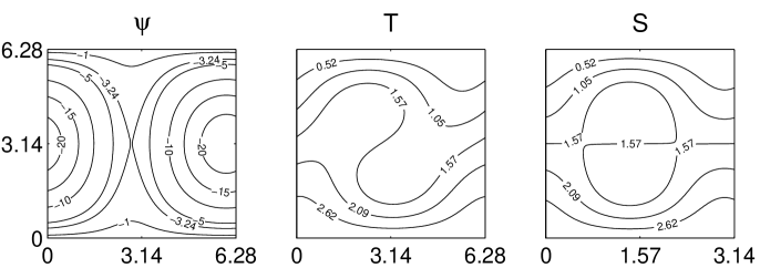
Figure 1: Stream function, temperature and salinity fields of the steady solution for $\sigma=10^{-2}$, $\tau=10^{2}$, $R_{T}=-200$, $R_{S}=-400$. The fields are periodic in the horizontal. One period is shown.

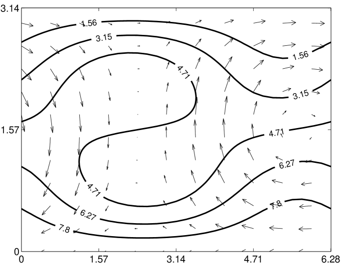
Figure 2: Density (solid line) and velocity field (arrows) for the flow of fig. 1. The density field is defined as: $\rho=T+(R_{S}/R_{T})S$.

When $A$ is small (we used $A=10^{-4}$) the nonlinearities are initially negligible, and the initial perturbation evolves quickly into a good approximation to the fastest growing eigenfunction. As the nonlinear terms become important, the system settles to a steady solution, shown in figure 1. This solution is dominated by a large scale shearing velocity, sustained by a single convective cell, which, in our example, circulates in the clockwise direction. The reflected configuration with an anti-clockwise cell is also possible and is obtained by starting with a negative amplitude. The most remarkable feature of this solution is its steady, stable density inversion, associated with a saddle point in the stream function (cf. fig. 2). The formation of this structure, an incomplete wave roll-up, is preceded by a temporal development that begins in the linear stages of the growth with a pair of cells of opposite signs, as in ordinary convection. This motion induces a wave pattern in the temperature and salinity fields. When the amplitudes $W^{+}$ and $W^{-}$ reach the order of unity, the onset of the large scale flow $U$ makes the convective cells more and more asymmetrical, advecting the temperature and salinity wave crests close to each other as they encroach on the weaker cell, and stretching them apart in the stronger one. Finally, the weaker cell disappears altogether, leaving a tongue of warm, salty fluid folded over a tongue of cold, fresh fluid, above a saddle point in the stream function, in a remarkable advective-diffusive equilibrium. Further simulations show that this is a stable solution.

We also performed a run where the absolute values of the Rayleigh numbers were slowly and continuously lowered at the rate of $(1.5\cdot 10^{-6})$ units per thermal time, while keeping their ratio constant. The steady solution survives up to $R_{T}\approx-14.5$ when it abruptly falls to the conductive state, supporting the supposition that it appears through a sub-critical bifurcation.

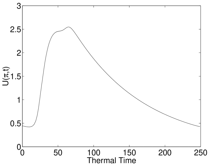
Figure 3: Time evolution of the shearing velocity $U$ at $z=\pi$.

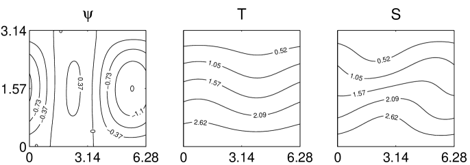
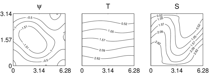
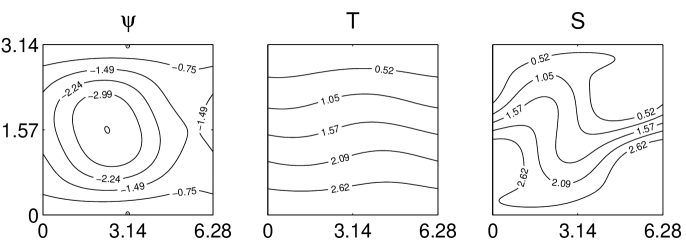
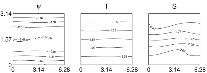
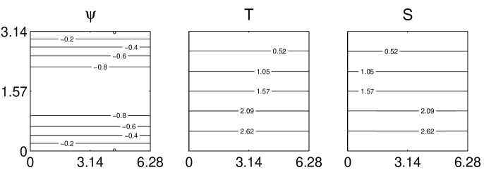
Figure 4: Stream function, temperature and salinity fields during the cycle of Fig. 3. They correspond to the times (from top to bottom): $t=14$, $t=24$, $t=48$, $t=63$, $t=163$. The fields are periodic in the horizontal. One period is shown.

A completely different dynamics appears if one sets $A=1$ in the initial conditions. We then find a solution that proceeds in cycles of approximately $t_{c}\simeq 246$ thermal times. In figure 3 we show the time evolution of $U$ at $z=\pi$, during one such cycle. For convenience we set $t=0$ just before the large-scale flow reaches its minimum amplitude. At this time, the stream function shows a large, anti-clockwise cell, placed beside a smaller region of weak clockwise circulation. Growing, wave-like patterns shape the temperature and the salinity fields as they are advected across the domain by the large-scale flow (fig. 4, first panel from top). In this case, however, the shear is a leading order effect, and slows the growth of the overstable oscillations.

Shortly thereafter, the asymmetry of the convective cells drives up the amplitude of the large-scale flow. The second panel from the top of figure 4 shows the fields at time $t=24$. The stream function is dominated by a single, anti-clockwise cell. All clockwise circulation is confined to two small regions close to the upper and the lower boundary. Gradients in the salinity field increase, and the wave pattern is skewed. On the other hand, because the cell’s turnover time is of the same order as the thermal diffusivity time, the temperature field is only slightly perturbed.

At a later time, ($t=48$, fig. 4, third panel from top), the large scale flow is close to its maximum intensity. All clockwise circulation has disappeared from the stream function. A sequence of wave roll-ups has made the salinity field homogeneous over some parts of the domain, and it has greatly increased the gradients elsewhere. Notice the similarity between the stream function at this time and the stream function of the steady solution. In both cases, the circulation has the same sign in the whole domain, and the convective cells are separated by saddle points. Here, however, the strength of convection is weaker than in the steady solution. The flow is too slow to advect the temperature field appreciably, and the salinity plumes are too heavy to be sustained by the flow in a steady equilibrium.

The sequence of wave roll-ups continues until the shear becomes too intense to allow for any further roll-up ( $t=63$, fig. 4, fourth panel from top). At that point, the high shear disrupts the convective cells and destroys the inhomogeneities in the temperature and salinity fields, bringing them close to the conductive solution.

For the remaining fraction of the whole cycle, the flow is dominated by an intense, $x$-independent shear which flows rightward in the upper half of the domain, and leftward in the lower half ($t=163$, fig. 4, fifth panel from top). As for the steady case, for each solution there is a symmetric one with the shear flowing in the opposite direction; the particular choice of initial conditions selects between the two possibilities. The temperature and the salinity fields closely resemble the conductive solution $T=S=-z$. The amplitudes $W^{+}$, $W^{-}$, $\Theta^{+}$, $\Theta^{-}$, $\Phi^{+}$ and $\Phi^{-}$ are very small (less than $5\cdot 10^{-4}$ in our non-dimensional units) at any height $z$. The evolution of $U$ is essentially decoupled from the dynamics of the other variables, and it is reduced to a slow viscous decay. Finally, when the intensity of the shear has been sufficiently damped, the overstable oscillations restart their growth, and the cycle begins again.

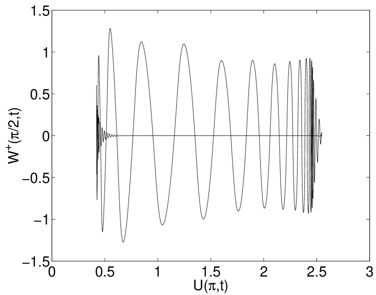
Figure 5: Shearing velocity $U$ at top boundary vs vertical velocity amplitude $W^{+}$ at the middle of the computational domain during the cycle of Fig. 3.

The dynamics that we just described is summarized in figure 5, where we plot the value of the shearing velocity $U$ at the top boundary versus the value of $W^{+}$ in the middle of the slab.

With the parameters discussed here, the cycles are not perfectly periodic. In fact, longer simulations reveal that the cyclic behavior is only a long transient. After approximately 4500 thermal times the flow falls back to the steady solution. On the other hand, at lower Rayleigh numbers, such as $R_{T}=-100$ and $R_{S}=-200$, the wave-shear mixing cycle appears to be a perfectly periodic solution. Further exploration of the parameter space has shown that, either as a transient or as the asymptotic regime, the roll-up of overstable oscillations by a self-excited shear is a behavior characteristic of the low Prandtl number regime.

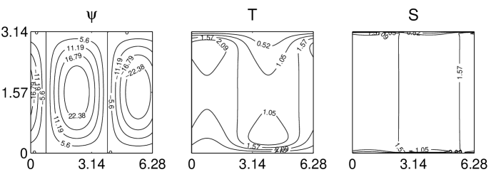
Figure 6: Stream function, temperature and salinity fields in the simulation with $U\equiv 0$. This is a steady solution. The fields are periodic in the horizontal. One period is shown.

In order to bring out the key role of the large-scale flow, we have carried out a simulation where the variable $U$ was kept equal to zero at all times, which is equivalent to removing the first of the equations (3). Starting from initial conditions of small amplitude, the numerical solution undergoes an oscillatory instability in agreement with the predictions of the linear analysis. However, after about 100 thermal times the solution has converged to a steady state, shown in figure 6. In this solution, all the salinity gradients are concentrated at the boundaries. In the interior of the domain the salinity is almost constant. This brings the system to a state analogous to purely thermal convection without shear, with two symmetric cells in the stream function field, and two steady thermal plumes (one ascending, the other descending) in steady equilibrium between advection and diffusion.

3.2 A Lagrangian view of the wave-shear mixing.

The numerical simulations described above show that the fluid can alternate long periods of laminar motion with relatively shorter times of tumultuous overturning. To better investigate the details of these mixing events we have computed the trajectories of a sample of fluid particles. For this purpose, the variables $U$, $W^{+}$ and $W^{-}$ are interpolated using cubic spines (taking care to use the correct boundary conditions in their spline representation), to recover the fluid velocity $\mathbf{u}_{i}(x,z)$ at the position of the $i$-th particle. The advection equation $\dot{\mathbf{x}}_{i}=\mathbf{u}_{i}$ is then integrated at each Eulerian time step with a second order Adams-Bashfort scheme to obtain the particles’ trajectories.

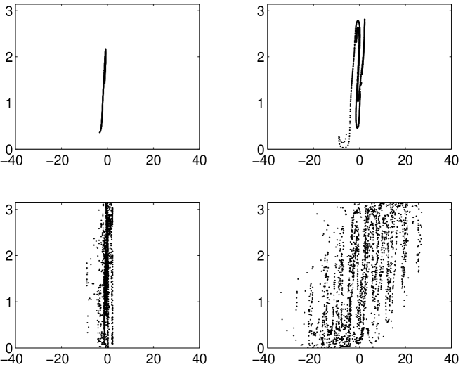
Figure 7: Positions of 2500 Lagrangian tracers at different times. From left to right, top to bottom: $t=15$; $t=20$; $t=25$; $t=30$. The tracers were released at time $t=0$ (cf. Fig. 3).

We release 2500 particles at time $t=0$ on a square array of 50 by 50 points, with side length of 0.5 non-dimensional units, and with the lower left corner at (0, $\pi/3$). As time goes on, the first part of each thermohaline oscillation stretches the ensemble of particles vertically, the large-scale flow slants it, and the second part of the oscillation folds it. The interplay of waves and shear produces a dynamics very similar to that of a Baker’s map, and it is pictured in the time sequence of figure 7 (for an introduction to the physics of mixing see Ottino (1989); a simple example of such mixing flow is given by Aref’s blinking vortex, Aref, 1984). The stretching and folding continues until the thermohaline oscillations are disrupted by the shearing velocity. By the time $U$ reaches its maximum amplitude, ($t\simeq 65$), the distribution of tracers has become vertically homogeneous.

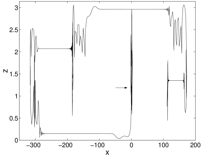
Figure 8: Trajectory of a single Lagrangian tracer. The path begins at the position marked by the arrow. The integration lasts for 1000 thermal times. Four mixing events, and the beginning of a fifth, are clearly visible, alternated with periods where the advection is only along the $x$-axis.

The trajectory of an individual Lagrangian tracer (cf. fig. 8 ) illustrates what happens on longer time scales. The mixing events are clearly singled out by the periods of wiggly motion, alternating with periods where the advection is due to only the large scale velocity $U$. Since the sign of the shear remains constant, when a Lagrangian tracer happens to be in the upper half of the computational domain, it travels rightward, while it travels leftward when in the lower half. Dispersion in the horizontal direction occurs because the $z$ coordinate of a particle after a mixing event has a sensitive dependence upon the particle’s position before the mixing event. Each particle switches in an unpredictable way between rightward and leftward motion, performing a random walk along the $x$-axis. Thus we expect the horizontal transport of particles to be described by a diffusion process. On a dimensional basis, we can express its diffusion coefficient as $K=U_{c}^{2}t_{c}$. We estimate $U_{c}$ as the time and space average of $|U|$ and $t_{c}$ as the duration of the viscous decay of the shearing velocity that separates a mixing event from the next. In our non-dimensional units we have $U_{c}\approx 0.85$, $t_{c}\approx 180$, which yields $K\approx 130$.

This qualitative description is confirmed by evaluating the single-particle dispersion $\xi^{2}$

$$\xi^{2}(t;\mathbf{x}_{i}(t_{0}))=\frac{1}{N}\sum_{i=1}^{N}\left|\mathbf{x}_{i}(t)-\mathbf{x}_{i}(t_{0})\right|^{2}$$ (5)

where $N$ is the number of Lagrangian tracers and $\mathbf{x}_{i}(t_{o})$ is the initial position of the $i$-th one. In the case of Brownian motion, $\xi^{2}$ does not depend on the initial positions and it is related to the diffusion coefficient $K$ of the Brownian stochastic process by the formula $\xi^{2}(t)=2Kt$ (Gardiner, 1996). In our case, since the Eulerian flow has very different characteristics along the $x$ and the $z$ direction, we apply the definition of single-particle dispersion separately to each direction.

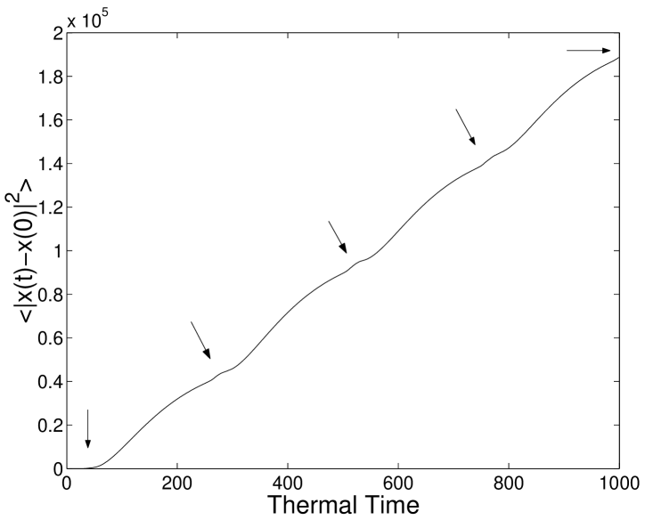
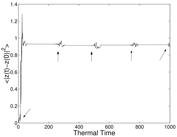
Figure 9: Single-particle dispersion along the horizontal (left panel) and the vertical (right panel). The times when sequences of wave roll-ups (mixing events) occur are marked by the arrows.

The results are shown in figure 9. The overall trend of $\xi^{2}(t)$ for horizontal displacements is well approximated by a linear fit, which gives an effective diffusion coefficient $K=98.6\pm 1.0$ in non-dimensional units, in good agreement with the above rough estimate. However, on short time scales, the behavior of $\xi^{2}(t)$ is not perfectly linear. Initially, in the $x$-direction, dispersion grows slowly, because the tracers are all clustered together into a single, coherent convection cell. After the first vertical mixing event (marked by the arrow in figure 9), the horizontal dispersion grows faster with time. At this stage, the dispersion is approximately ballistic (that is $\xi^{2}\propto t^{2}$) until $U$ can be approximated by a constant. However, as the large scale flow $U$ decays, the dispersion slows down as well, until the next mixing event occurs.

Along the vertical direction, the single-particle dispersion grows from zero to its maximum value during the first occurrence of wave-rollups, which makes the tracers’ distribution homogeneous in the vertical. The vertical dispersion then remains approximately constant, with statistical fluctuations during the vertical mixing events.

To confirm that the flow of figure 4 produces authentic mixing, we look for evidence that particle paths are independent of each other by evaluating the pair dispersion $\Xi^{2}$

$$\Xi^{2}(t)=\frac{2}{N(N-1)}\sum_{i=1}^{N}\sum_{j>i}\left|\mathbf{x}_{i}(t)-\mathbf{x}_{j}(t)\right|^{2}.$$ (6)

If each particle follows an independent Brownian path, then $\Xi(t)=4Kt$. On evaluating the diffusion coefficient along the $x$-direction by using pair dispersion, we find $K=102.0\pm 1.0$, in close agreement with the value obtained in the single particle analysis. This is strong evidence that the long-time transport properties of the flow in the horizontal direction are those of Brownian motion, and can thus be modeled by a suitable eddy diffusion coefficient.

We carried out a similar simulation for the case where the large-scale flow is not allowed. As expected when the Eulerian flow is steady, the tracers moved along periodic orbits. Even after 1000 thermal times the 2500 tracers, seeded at the same initial position as the tracers in the simulation described above, remain confined in a circular belt and do not disperse.

To complement the information given by the advection of individual Lagrangian tracers, and to give a further visual indication that no barriers to mixing exist in the flow of figure 4, we carried out some simulations in which we use the streamfunction generated by our model to advect a passive scalar field $c$, according to the equation

$$\partial_{t}c-J(\psi,c)=\frac{\kappa_{c}}{\kappa_{T}}\nabla^{2}c.$$ (7)

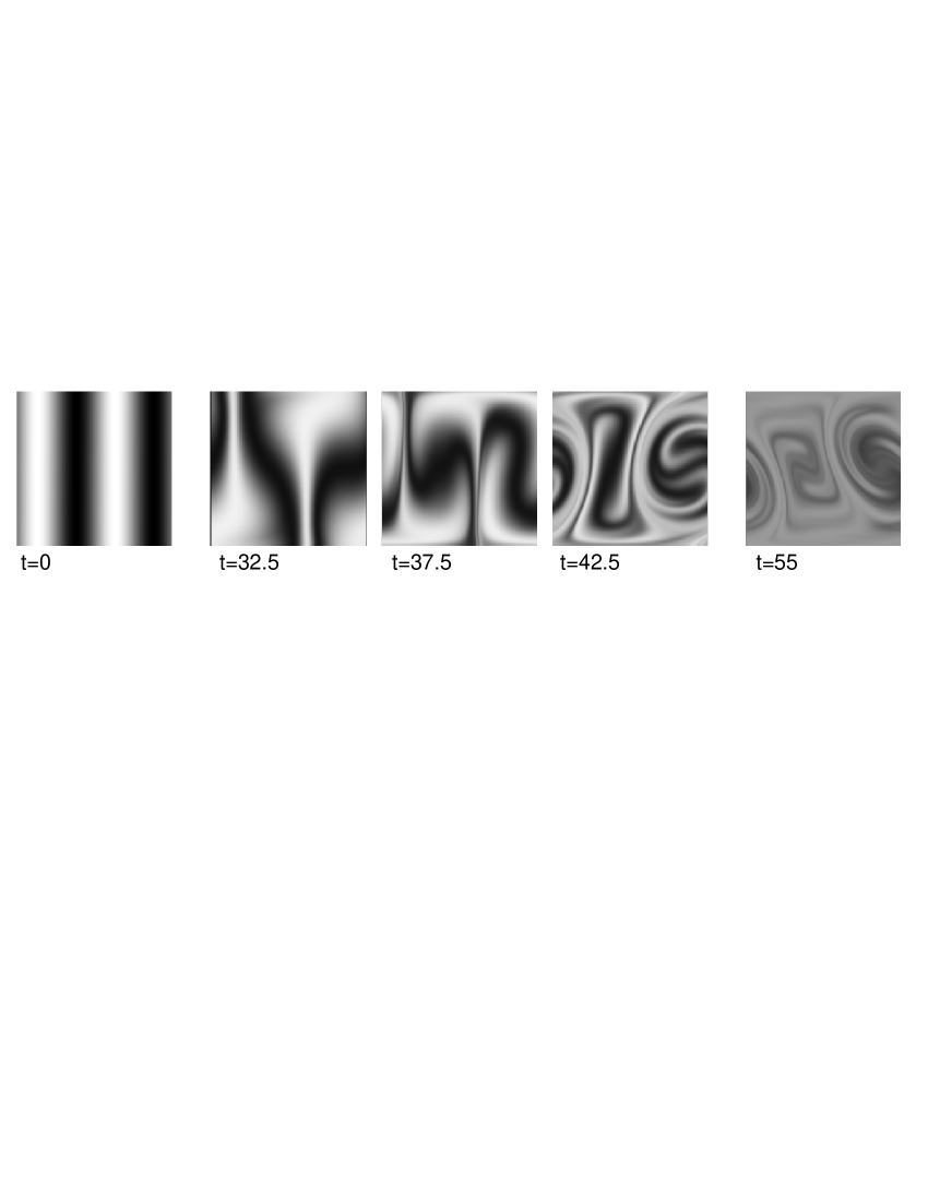
Figure 10: Evolution of the concentration of a passive scalar during a complete cycle of the flow in figure 4. The grey scale is between 0 and 1. The transition from oscillation to direct convection is visible in the 3 central panels whereas the last one shows how much homogenization occurred during one cycle. The fields are periodic in the horizontal. One period is shown.

The small amount of diffusion $\frac{\kappa_{c}}{\kappa_{T}}=0.001$ is necessary in order to maintain the stability of the finite volume code used to integrate equation (7). Figure 10 shows a time sequence of the numerical solution, and illustrates the high degree of homogeneity reached by the passive scalar during a single wave-shear mixing cycle.

4 ODD convection with heat and salt.

Because conditions favoring the onset of ODD convection occur at several places in the Earth’s oceans we investigate the behavior of the model in the parameter range appropriate for sea water. For this, we adopt $\sigma=10$, and $\tau=10^{2}$, which are approximately the values of the Prandtl and the Lewis numbers of sea water. With these parameters, the ODD instability occurs when the density ratio $R_{\rho}={R_{T}}/{R_{S}}$ approaches unity (Baines & Gill, 1969).

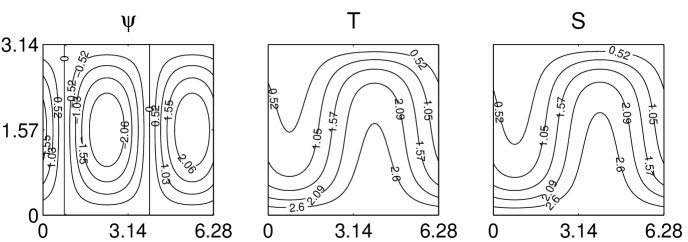
Figure 11: Stream function, temperature and salinity fields for the heat and salt simulation with $R_{T}=-200$ and $R_{\rho}=0.99$. The fields are periodic in the horizontal. One period is shown.

When $R_{T}=-200$, $R_{\rho}=0.99$ the system converges to a limit cycle characterized by a pair of plumes which oscillate up and down as standing waves, with periods of $\simeq 0.61$ thermal times. Figure 11 shows a snapshot of the stream function, temperature and salinity fields close to the extremum of one oscillation: the warm, salty plume on the right has just reached the maximum elevation, the cold, fresh plume on the left has reached its maximum depth, and they are both moving back toward the middle of the domain. The large scale flow is not excited, and initial perturbations on $U$ decay as $e^{-\sigma t}$. No Lagrangian mixing occurs in this simple flow.

Searching for a self-excited large-scale flow, we increased the Rayleigh number up to $R_{T}=-1000$, and we have set the density ratio to $R_{\rho}=0.95$. To accurately resolve the high salinity gradients that develop at the top and bottom boundaries, we increased the vertical resolution to 256 modes. The initial conditions are the same as in section 3.1. We have tried several values for the initial amplitude $A$ in the range $[10^{-3},10]$. The solution that we find exhibits extremely long cycles of approximately $100$ thermal times, independently of the value of $A$.

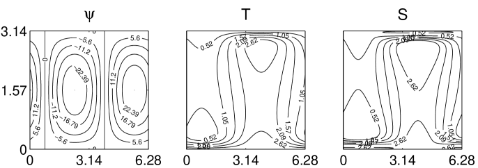
Figure 12: Streamfunction, temperature and salinity fields for the heat and salt simulation with $R_{T}=-1000$ at time $t=4.3$. The phase of the oscillation is the same as in figure 11 The fields are periodic in the horizontal. One period is shown.

Initially this solution shows a pair of oscillating plumes analogous to those found at $R_{T}=-200$. They move faster (the period of oscillation is 0.3 thermal times, but it shrinks as the amplitude of the oscillations grows), and lead to sharper gradients in the scalar fields. The large-scale flow is excited, but it is so weak that the associate skewness of the convective cells is imperceptible in the figures. Figure 12 shows the stream function, the temperature and the salinity fields for the simulation starting with $A=0.01$ at time $t=4.3$, when the salinity fluctuations reach their maximum amplitude. The oscillations, however, do not last indefinitely as in the previous case. They damp out in a few thermal times, and the motion in the fluid ceases almost completely.

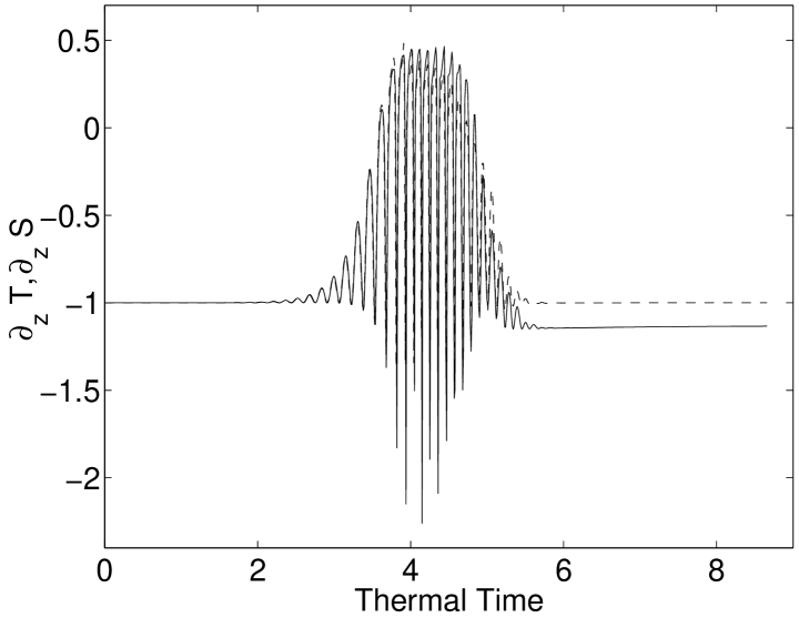
Figure 13: Time evolution of $\partial_{z}\overline{T}$ (dashed line) and $\partial_{z}\overline{S}$ (solid line) computed at $z=\pi/2$ in the simulation with $R_{T}=-1000$ .

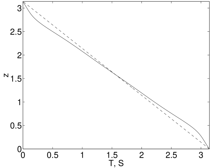
Figure 14: Horizontally averaged temperature (dashed line) and salinity (solid line) in the simulation with $R_{T}=-1000$ at the time $t=4$.

By looking at the vertical profiles of temperature and salinity it is possible to find a hint of the mechanism that switches off the oscillations. Figure 13 shows the time evolution of $\partial_{z}\overline{T}$ and $\partial_{z}\overline{S}$ computed at $z=\pi/2$ (that is, in the middle of the slab). Initially $\partial_{z}\overline{T}=\partial_{z}\overline{S}=-1$. As the doubly-diffusive oscillations grow and then damp out, the slope of the salinity profile becomes steeper than the slope of temperature, and one is left with $\partial_{z}\overline{S}<-1$, while the temperature slope promptly returns to the diffusive solution $\partial_{z}\overline{T}=-1$. This results in a decreased density ratio in the middle of the slab, which locally makes the fluid linearly stable. Figure 14 shows the horizontally averaged profiles of temperature and salinity at the time $t=6$. The density ratio at $z=\pi/2$ is now $R_{\rho}=\frac{\partial_{z}\overline{T}}{\partial_{z}\overline{S}}R_{\rho_{\rm initial}}=0.831$, which is less than the critical value $R_{\rho_{\rm critical}}=0.9163\ldots$ required to have a linear instability for the chosen values of $R_{T}$, $\sigma$, and $\tau$. At this time all motion has become negligibly small. The only dynamic in the system is the slow diffusion of the salinity field, which relaxes to the conductive solution with a time scale which, in non dimensional units is $O(\tau)$. Finally, when $t\approx 100$, the growth of ODD instability resumes and the whole cycle starts over with an alternation of short-lived oscillatory convection and slow diffusive relaxation. This dynamics does not lead to mixing. A set of Lagrangian tracers seeded in the way described in section 3.2 remains closely packed during the whole duration of the oscillations.

While the salinity build-up stabilizes the bulk of the fluid, we observe in figure 14 that, near the boundaries, $\partial_{z}\overline{T}<\partial_{z}\overline{S}$, implying that the fluid there is unstably stratified. However, we do not observe direct convection being triggered at the boundaries. We assume that this is a consequence of the truncation of the Boussinesq equations (1): the range of horizontal wavenumbers which would be unstable is not represented in the truncated model (3). Numerical solutions of the untruncated equations are needed in order to show whether convection actually arises at the boundaries and in what ways it contributes to the establishment of the step-like profiles seen in laboratory experiments (Huppert & Linden, 1979).

In this simulation the large-scale flow $U$ does not seem to play a dominant role. The doubly-diffusive oscillations are suppressed by the salinity build-up in the center of the domain, and not by the shear induced by $U$, as in the low Prandtl number case. Indeed, a simulation with $R_{T}=-500$ and $R_{\rho}=0.95$ shows the same qualitative dynamics as the simulations with $R_{T}=-1000$, but there is no self-excitation of a large-scale flow.

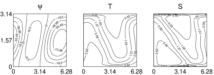
Figure 15: Streamfunction, temperature and salinity fields at time $t=4.3$ for the heat and salt simulation with $R_{T}=-1000$ and an externally imposed shear $\omega_{0}=0.2$. The fields are periodic in the horizontal. One period is shown.

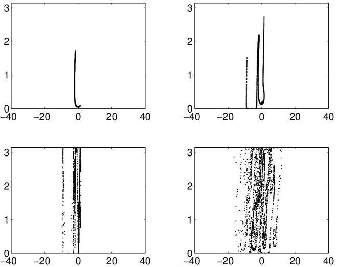
Figure 16: Positions of 2500 Lagrangian tracers at different times in a simulation with sea water parameters and an externally imposed shear. From left to right, top to bottom: $t=4$; $t=4.15$; $t=4.3$; $t=4.45$.

However, large-scale flows are prevalent in geophysics where they need not be convectively driven. Such flows may play the kind of role in the convective process that the shears we have been discussing do. For this reason, we have investigated the interaction between ODD oscillations and an imposed shearing velocity, $U=\widetilde{U}+\omega_{0}z$ in the equations (3), and solving for $\widetilde{U}$. Here $\omega_{0}$ is a constant shear. In our spectral code we represent $z$ as a trigonometric sum in the interval $[0,\pi]$, truncated at the Nyquist frequency. We keep $R_{T}=-1000$, $R_{\rho}=0.95$, and we impose an external shear $\omega_{0}=0.2$. Once again, oscillating plumes develop as a result of the ODD instability. The presence of the external shear makes the convective cells sufficiently asymmetric that they now can contribute to the build-up of a large-scale flow, which can reach a peak intensity of $30$ non dimensional units close to the boundaries. A snapshot of the fields at time $t=4.3$ is shown in figure 15. As in the case with low Prandtl number, the large-scale flow induces wave roll-ups, which mix the fluid until the salinity build-up chokes the motion. The resulting Lagrangian chaos is illustrated in figure 16.

5 Discussion and conclusions

This exploratory study of sheared ODD convection has revealed some previously unknown phenomenology. The main finding is that the presence of a large-scale shearing velocity (be it self-excited or externally imposed) induces vigorous mixing. The mechanism is reminiscent of the mixing induced by the Baker’s map: ODD waves vertically stretch material lines, the shear slants them, so that they can subsequently be folded up. This engenders a rapid, effective homogenization of Lagrangian tracers along the vertical. Horizontal mixing is also enhanced, in a way which recalls the phenomenon of shear dispersion (see, e.g. Jones & Young, 1994). As first noticed by Taylor, in the presence of a shear, molecular diffusion is enhanced along the direction of the flow. In our model the wave-shear mixing plays the role of molecular diffusion.

Further work is needed to asses at which Rayleigh numbers the large-scale flow appears. Spontaneous generation of shear seems very elusive at high Prandtl number, as in the case of heat and salt in water. This is supported by the laboratory experiments of Stamp & Griffiths (1997) and Stamp et al. (1998). They observe the generation of large-scale flows in convecting regions above and below an interface having ODD-favorable stratification (therefore giving further indication that this is a common feature of convecting fluids). The flows have the same intensity and direction above and below the interface, so they do not cause any shear on the interface, but merely translate it, either leftward or rightward. In an annular geometry, in the reference frame comoving with the mean flow, they observe gross features in agreement with the results on step-like interfaces of Gough & Toomre (1982), who employ a truncated model similar to ours.

On the other hand, we find that large-scale shearing flow is easily generated at very low Prandtl number, which is of interest in astrophysical applications. Unfortunately, carrying out either laboratory experiments or reliable direct numerical simulations in this regime is challenging. Other mechanisms can lead to mixing, distinct from that illustrated in this work. In particular, the simulations of Merryfield (1995) and of Biello (2001) both show ODD oscillations breaking into small-scale turbulence, as in the earlier discussion of Stevenson (1979). A larger investigation is needed to decide which of these mechanisms may be the more significant in different contexts.

In all cases where we have found mixing-inducing motion, it lasts for a relatively short interval, and it is then followed by a longer interval of non-mixing dynamics. The physical cause of this intermittent behavior is different in the low Prandtl number regime and in the sea water regime. In the first case the stabilizing factor is the shearing velocity $U$; in the second case the fluid is made linearly stable by a salinity build-up away from the boundaries. The present study has suggested that the astrophysical situation is the one in which the convectively induced shears come into play. This points to the value of a study directed at low Prandtl number ODD convection and suggests that we next seek simplifications that may help us in that limit.

References

- (1) Aref, H. “Stirring by chaotic advection”, J. Fluid Mech., 143, 1, (1984).
- (2) Baines, P. G. and Gill, A. E., “On thermohaline convection with linear gradients”, J. Fluid Mech., 37, 289, (1969).
- (3) Biello, J. A., “Layer formation in semiconvection”, preprint: astro-ph/0102338, http://arXiv.org/abs/astro-ph/0102338.
- (4) Da Costa, L.N., Knobloch, E. and Weiss, N.O., “Oscillations in double-diffusive convection”, J. Fluid Mech., 109, 25-43 (1981).
- (5) Franceschini, V. and Tebaldi, C., “Truncations to 12, 14 and 18 modes of the Navier-Stokes equations on a two-dimensional torus”, Meccanica, 20, 207, (1985).
- (6) Gardiner, C. W., “Handbook of Stochastic Methods”, II edition, Springer-Verlag, Berlin (1996).
- (7) Gough, D. O., Spiegel, E. A. and Toomre, J., “Modal equations for cellular convection”, J.Fluid Mech., 68, 695, (1975).
- (8) Gough, D. O. and Toomre, J., “Single-mode theory of diffusive layers in thermohaline convection”, J.Fluid Mech., 125, 75, (1982).
- (9) Howard, L. N., and Krishnamurti, R., “Large scale flow in turbulent convection: a mathematical model”, J. Fluid Mech., 170,385, (1986).
- (10) Huppert, H. E. and Linden, P. F., “On heating a stable salinity gradient from below”, J. Fluid Mech., 95, 431, (1979).
- (11) Jacobs, C. A., Huppert, H. E., Holdsworth, G. and Drewy, D. J., “Thermohaline steps induced by melting at the Erebus Glacier tongue”, J. Geophys. Res., 86, 6547, (1981).
- (12) Jones, S. W. and Young, W.R., “Shear dispersion and anomalous diffusion by chaotic advection”, J. Fluid Mech.,280, 149, (1994).
- (13) Kolodner, P. R., Glazier, J. A. and Williams, H. L., “Dispersive Chaos in One-Dimensional Traveling-Wave Convection”, Phys. Rev. Lett., 65, 1579, (1990).
- (14) Krishnamurti, R. and Howard, L. N., “Large scale flow in turbulent convection”, Proc. Natl. Acad. Sci. USA, 78, 1981, (1981).
- (15) Marmorino, G. O., “Intrusions and diffusive interfaces in a salt fingering staircase”, Deep-Sea Research, 38, 1431, (1991).
- (16) Merryfield, W. J., “Hydrodynamics of Semiconvection”, Astrophys. J., 444, 318, (1995).
- (17) Neal, V. T., Neshiba, S. and Denner, W., “Thermal stratification in the Arctic Ocean”, Science, 166, 373, (1969).
- (18) Ottino, J. M., “The Kinematics of Mixing: Stretching, chaos, and transport”, Cambridge University Press, Cambridge (1989).
- (19) Paparella, F. and Spiegel, E. A., “Sheared salt fingers: Instability in a truncated system”, Phys. Fluids, 11, 1161, (1999). (PS)
- (20) Ruddick, B., “Intrusive mixing in a Mediterranean salt lens – Intrusion slopes and dynamical mechanisms”, J. Phys. Oceanogr., 22, 1274, (1992).
- (21) Siggia, E. D., “High Rayleigh Number Convection”, Annu. Rev. Fluid Mech, 26, 137, (1994).
- (22) Spiegel, E. A., “Semiconvection”, Comments on Ap. and Space Physics, 1, 57, (1969).
- (23) Stamp, A. P., Hughes, G. O., Nokes, R. I. and Griffiths, R. W., “The coupling of waves and convection”, J. Fluid Mech., 372, 231, (1998).
- (24) Stamp, A. P. and Griffiths, R. W., “Turbulent traveling-wave convection in a two-layer system”, Phys. Fluids, 9, 963, (1997).
- (25) Stevenson, D. J., “Semiconvection as the occasional breaking of weakly amplified internal waves”, Monthly Not. Royal Astr. Soc., 187, 129, (1979).
- (26) Turner, J. S., “Buoyancy effects in fluids”, Cambridge University Press, Cambridge (1979).
- (27) Veronis, G., “On finite amplitude instability in thermohaline convection”, J. Marine Res., 23, 1, (1965).