Combining cosmological datasets: hyperparameters and Bayesian evidence

Abstract

A method is presented for performing joint analyses of cosmological datasets, in which the weight assigned to each dataset is determined directly by it own statistical properties. The weights are considered in a Bayesian context as a set of hyperparameters, which are then marginalised over in order to recover the posterior distribution as a function only of the cosmological parameters of interest. In the case of a Gaussian likelihood function, this marginalisation may be performed analytically. Calculation of the Bayesian evidence for the data, with and without the introduction of hyperparameters, enables a direct determination of whether the data warrant the introduction of weights into the analysis; this generalises the standard likelihood ratio approach to model comparison. The method is illustrated by application to the classic toy problem of fitting a straight line to a set of data. A cosmological illustration of the technique is also presented, in which the latest measurements of the cosmic microwave background power spectrum are used to infer constraints on cosmological parameters.

1 Introduction

It is now common practice in cosmology to estimate the values of cosmological parameters by a joint analysis of a number of different datasets. The standard technique for performing such an analysis is to assume that the datasets are statistically independent and so take the joint likelihood function for the parameters to be given simply by the product of the individual likelihood functions for each separate dataset. The joint likelihood function can then be used in the standard way to determine the optimal values of the parameters and their associated errors.

As discussed by Lahav et al. (2000; hereinafter Paper I), however, there exists some freedom in the relative ‘weight’ that may be given to each dataset in the analysis (see also Godwin & Lynden-Bell 1987; Press 1996). The assignment of weights often occurs when two or more of the datasets are inconsistent, and is usually made in a somewhat ad-hoc manner. Typically some datasets are excluded from the analysis, and hence given a weight of zero, while the remainder are analysed jointly with equal weights. Despite its widespread use, this procedure has many unsatisfactory features, not least of which is the subjectivity associated with the choice of which datasets to include, and which to discard. As advocated in Paper I, a more objective procedure for assigning weights to the datasets is provided by the introduction of hyperparameters. This device allows the statistical properties of the data themselves to determine the weight given to each dataset in the analysis.

In Paper I, a method was presented for introducing hyperparameters into the analysis of datasets for which each likelihood function had a particular simple form. This technique was then applied to the estimation of the Hubble parameter $h$ from several sets of observations of the power spectrum of cosmic microwave background (CMB) anisotropies. It was shown that apparently discrepant datasets could be analysed jointly to provide a consistent estimate of $h$, together with an associated error. This approach has also recently been applied to the joint analysis of the baryon mass fraction in clusters and cepheid-calibrated distances (Erdogdu, Ettori & Lahav 2002).

In this paper, we extend the work of Paper I to accommodate more general situations. In section 2, we review the standard approach to Bayesian parameter estimation and discuss the role of the Bayesian evidence in model selection. In section 3, we present a general account of hyperparameters and their use in joint estimation of parameters. We also discuss how to use the Bayesian evidence to decide whether or not the data support the inclusion of hyperparameters in the first instance. In section 4, we consider the use of hyperparameters in the weighting of datasets and, in section 5, we discuss the common special case in which the likelihood function for each dataset is Gaussian. In section 6, we illustrate the useful properties of the hyperparameters approach by applying the technique to the toy problem of fitting a straight-line to a number of datasets. A cosmological application of the hyperparameters approach is discussed in section 7, in which we perform a joint estimate of the physical baryon density $\Omega_{b}h^{2}$ and the scalar spectral index $n$ using the most recent sets of observations of the CMB power spectrum. Finally, our conclusions are presented in section 8.

2 Bayes’ theorem and evidence

Suppose the totality of our data is represented by the data vector D and we are interested in estimating the values of the parameters $\mn@boldsymbol{\theta}$ in some underlying model of the data. The standard approach to this problem is to use Bayes’ theorem

$$\Pr(\mn@boldsymbol{\theta}|{\textbf{{D}}})=\frac{\Pr({\textbf{{D}}}|\mn@boldsymbol{\theta})\Pr(\mn@boldsymbol{\theta})}{\Pr({\textbf{{D}}})},$$ (1)

which gives the posterior distribution $\Pr(\mn@boldsymbol{\theta}|{\textbf{{D}}})$ in terms of the likelihood $\Pr({\textbf{{D}}}|\mn@boldsymbol{\theta})$, the prior $\Pr(\mn@boldsymbol{\theta})$ and the evidence $\Pr({\textbf{{D}}})$ (which is also often called the marginalised likelihood).

2.1 Parameter estimation

For the purpose of estimating parameters, one usually ignores the normalisation factor $\Pr({\textbf{{D}}})$ in Bayes’ theorem, since it does not depend on the parameters $\mn@boldsymbol{\theta}$. Thus, one instead works with the ‘unnormalised posterior’

$$\overline{\Pr}(\mn@boldsymbol{\theta}|{\textbf{{D}}})\equiv\Pr({\textbf{{D}}}|\mn@boldsymbol{\theta})\Pr(\mn@boldsymbol{\theta}),$$ (2)

where we have written $\overline{\Pr}$ to denote the fact that the ‘probability distribution’ on the left-hand side is not normalised to unit volume. In fact, it is also common to omit normalising factors, that do not depend on the parameters $\mn@boldsymbol{\theta}$, from the likelihood and the prior. As we shall see below, however, if one wishes to calculate the Bayesian evidence for a particular model, the likelihood and the prior must be properly normalised such that $\int\Pr(\mn@boldsymbol{\theta})\,d\mn@boldsymbol{\theta}=1$ and $\int\Pr({\textbf{{D}}}|\mn@boldsymbol{\theta})\,d{\textbf{{D}}}=1$. We will therefore assume here that the necessary normalising factors have been retained.

Strictly speaking, the entire (unnormalised) posterior is the Bayesian inference of the parameters values. Unfortunately, if the dimension $M$ of the parameter space is large, it is often numerically unfeasible to calculate $\overline{\Pr}(\mn@boldsymbol{\theta}|{\textbf{{D}}})$ on some $M$-dimensional hypercube. Thus, particularly in large problems, it is usual to present one’s results in terms of the ‘best’ estimates $\hat{\mn@boldsymbol{\theta}}$, which maximise the (unnormalised) posterior, together with some associated errors. These errors are usually quoted in terms of the estimated covariance matrix

$${\textbf{{C}}}=\left[-\left.\nabla\nabla\ln\overline{\Pr}(\mn@boldsymbol{\theta}|{\textbf{{D}}})\right|_{\mn@boldsymbol{\theta}=\hat{\mn@boldsymbol{\theta}}}\right]^{-1}.$$ (3)

or as confidence limits on each parameter $a_{i}$ $(i=1,\ldots,M)$, obtained from the one-dimensional marginalised (unnormalised) posterior distributions

$$\overline{\Pr}(a_{i}|{\textbf{{D}}})=\int\overline{\Pr}(\mn@boldsymbol{\theta}|{\textbf{{D}}})\,d\check{\mn@boldsymbol{\theta}},$$ (4)

where $d\check{\mn@boldsymbol{\theta}}=da_{1}\cdots d\check{a}_{i}\cdots da_{M}$ denotes that the integration is performed over all other parameters $a_{j}$ $(j\neq i)$.

The estimates $\hat{\mn@boldsymbol{\theta}}$ are most often obtained by an iterative numerical minimisation algorithm. Indeed, standard numerical algorithms are generally able to locate a local (and sometimes global) maximum of this function even in a space of large dimensionality. Similarly, the covariance matrix of the errors can be found straightforwardly by first numerically evaluating the Hessian matrix $\nabla\nabla\overline{\Pr}(\mn@boldsymbol{\theta}|{\textbf{{D}}})$ at the peak $\mn@boldsymbol{\theta}=\hat{\mn@boldsymbol{\theta}}$, and then calculating (minus) its inverse.

2.2 Bayesian evidence and model selection

The standard technique outlined above produces inferences of the parameter values for a given model of the data, but it does not provide a mechanism for deciding which one of a set of alternative models is most suitable for describing the data. This problem may be addressed, however, using the Bayesian evidence $\Pr({\textbf{{D}}})$. Very readable introductions to this topic are given by Bishop (1995) and Sivia (1996).

Although the evidence term is usually ignored in the process of parameter estimation, it is central to selecting between different models for the data. For illustration, let us suppose we have two alternative models (or hypotheses) for the data D; these hypotheses are traditionally denoted by $H_{0}$ and $H_{1}$. Let us assume further that the model $H_{0}$ is characterised by the parameter set $\mn@boldsymbol{\theta}$, whereas $H_{1}$ is described by the set of parameters $\mn@boldsymbol{\phi}$. For the model $H_{0}$, the probability density for an observed data vector D is given by

$$\Pr({\textbf{{D}}}|H_{0})=\int\Pr({\textbf{{D}}}|\mn@boldsymbol{\theta})\Pr(\mn@boldsymbol{\theta})\,d\mn@boldsymbol{\theta},$$ (5)

where, on the left-hand side, we have made explicit the conditioning on $H_{0}$. Similarly, for the model $H_{1}$,

$$\Pr({\textbf{{D}}}|H_{1})=\int\Pr({\textbf{{D}}}|\mn@boldsymbol{\phi})\Pr(\mn@boldsymbol{\phi})\,d\mn@boldsymbol{\phi}.$$ (6)

In either case, we see that the evidence is given by the average of the likelihood function with respect to the prior. Thus, a model will have a larger evidence if more of its allowed parameter space is likely, given the data. Conversely, a model will have a small evidence if there exist large areas of the allowed parameter space with low values of the likelihood, even if the likelihood function is strongly peaked and the corresponding model predictions agree closely with the data. Hence the value of the evidence naturally incorporates the spirit of Ockham’s razor: a simpler theory, having a more compact parameter space, will generally have a larger evidence than a more complicated theory, unless the latter is significantly better at explaining the data.

The question of which is the models $H_{0}$ and $H_{1}$ is prefered is thus answered simply by comparing the relative values of the evidences $\Pr({\textbf{{D}}}|H_{0})$ and $\Pr({\textbf{{D}}}|H_{1})$. The hypothesis having the larger evidence is the one that should be accepted. Although not widely used in cosmology, the idea of model selection using evidence ratios has been considered previously in this context by Jaffe (1996) and, more recently, by John & Narlikar (2001).

2.3 The Gaussian approximation to the posterior

Unfortunately, the evaluation of an evidence integral, such as (5), is a challenging numerical task. From (2), we see that

$$\Pr({\textbf{{D}}}|H_{0})=\int\overline{\Pr}(\mn@boldsymbol{\theta}|{\textbf{{D}}})\,d\mn@boldsymbol{\theta},$$ (7)

and so the evidence may only be evaluated directly if one can calculate $\overline{\Pr}(\mn@boldsymbol{\theta}|{\textbf{{D}}})$ over some hypercube in parameter space, which we noted earlier is often computational unfeasible. Nevertheless, if the data are conclusive, we would expect this (unnormalised) posterior to be sharply peaked about the position of the maximum $\mn@boldsymbol{\theta}=\hat{\mn@boldsymbol{\theta}}$. In this case, we may approximate this function by performing a Taylor expansion about $\mn@boldsymbol{\theta}=\hat{\mn@boldsymbol{\theta}}$. Working with the log-posterior, and keeping only terms up to second-order in $\mn@boldsymbol{\theta}$, leads to the Gaussian approximation of the (unnormalised) posterior distribution, which reads

$$\overline{\Pr}(\mn@boldsymbol{\theta}|{\textbf{{D}}})\approx\overline{\Pr}(\hat{\mn@boldsymbol{\theta}}|{\textbf{{D}}})\exp\left[-{\textstyle\frac{1}{2}}(\mn@boldsymbol{\theta}-\hat{\mn@boldsymbol{\theta}})^{\rm T}{\textbf{{C}}}^{-1}(\mn@boldsymbol{\theta}-\hat{\mn@boldsymbol{\theta}})\right],$$ (8)

where ${\textbf{{C}}}^{-1}$ is the estimated inverse covariance matrix of the parameters and is given by

$${\textbf{{C}}}^{-1}=-\left.\nabla\nabla\ln\Pr(\mn@boldsymbol{\theta}|{\textbf{{D}}})\right|_{\mn@boldsymbol{\theta}=\hat{\mn@boldsymbol{\theta}}}=-\left.\nabla\nabla\ln\overline{\Pr}(\mn@boldsymbol{\theta}|{\textbf{{D}}})\right|_{\mn@boldsymbol{\theta}=\hat{\mn@boldsymbol{\theta}}}.$$ (9)

Substituting the form (8) into (7), we thus find that an approximation to the value of the evidence is given by

$$\Pr({\textbf{{D}}}|H_{0})\approx(2\pi)^{M/2}|{\textbf{{C}}}|^{1/2}\,\Pr(\hat{\mn@boldsymbol{\theta}})\Pr({\textbf{{D}}}|\hat{\mn@boldsymbol{\theta}})$$ (10)

where $M$ is the number of parameters of interest $\mn@boldsymbol{\theta}$ and we have rewritten $\overline{\Pr}(\hat{\mn@boldsymbol{\theta}}|{\textbf{{D}}})$ using (2). Since the estimation of parameter values and their associated errors already requires one to calculate all the quantities on the right-hand side of (10), we see that this approximate evidence may be evaluated with no extra work. We note, however, that for (10) to hold, the prior and likelihood must be correctly normalised, such that $\int\Pr(\mn@boldsymbol{\theta})\,d\mn@boldsymbol{\theta}=1$ and $\int\Pr({\textbf{{D}}}|\mn@boldsymbol{\theta})\,d{\textbf{{D}}}=1$. We also note, in this case, that consideration of the ratio of evidences is a natural generalisation of the standard likelihood-ratio approach to model comparison.

2.4 Markov-Chain Monte-Carlo methods

We note, in passing, that the approach to parameter estimation and the approximate evaluation of evidences outlined above may soon become obsolete. With the advent of faster computers and efficient algorithms, it has recently become numerically feasible to sample directly from the posterior distribution using Monte-Carlo Markov-Chain (MCMC) techniques (see Knox, Christensen & Skordis 2001). This allows one trivially to obtain one-dimensional marginalised posteriors for each parameter of interest $a_{i}$, and also enables the direct numerical evaluation of evidence integrals. Clearly, the MCMC technique has enormous potential for the future estimation of cosmological parameters.

3 Hyperparameters

In this paper, we wish to construct a robust technique for performing a joint estimation of cosmological parameters from combined datasets. The basic idea behind the approach presented here is to introduce additional hyperparameters $\mn@boldsymbol{\alpha}$ into the Bayesian inference problem. In other words, we extend our parameter vector to include not only the parameters of interest $\mn@boldsymbol{\theta}$, but also the hyperparameters $\mn@boldsymbol{\alpha}$. These hyperparameters are analogous to ‘nuisance’ parameters that often arise in the standard approach to parameter estimation. In our case, however, they are not present in our model a priori, but we have chosen to introduce them in order to allow extra freedom in the parameter estimation process.

3.1 Marginalisation over hyperparameters

As with any set of nuisance parameters, we must integrate out (or marginalise over) the hyperparameters $\mn@boldsymbol{\alpha}$ in order to recover the posterior distribution of our parameters of interest $\mn@boldsymbol{\theta}$. Thus, we have

$$\Pr(\mn@boldsymbol{\theta}|{\textbf{{D}}}) = \int\Pr(\mn@boldsymbol{\theta},\mn@boldsymbol{\alpha}|{\textbf{{D}}})\,d\mn@boldsymbol{\alpha}$$ (11)

$$= \frac{1}{\Pr({\textbf{{D}}})}\int\Pr({\textbf{{D}}}|\mn@boldsymbol{\theta},\mn@boldsymbol{\alpha})\Pr(\mn@boldsymbol{\theta},\mn@boldsymbol{\alpha})\,d\mn@boldsymbol{\alpha}.$$

In this paper, we shall assume that the parameters of interest $\mn@boldsymbol{\theta}$ and the hyperparameters $\mn@boldsymbol{\alpha}$ are independent, so that

$$\Pr(\mn@boldsymbol{\theta},\mn@boldsymbol{\alpha})=\Pr(\mn@boldsymbol{\theta})\Pr(\mn@boldsymbol{\alpha}).$$ (12)

Substituting this form of the prior into (11), we immediately recover Bayes’ theorem (1), where the form of the likelihood function in the presence of hyperparameters is

$$\Pr({\textbf{{D}}}|\mn@boldsymbol{\theta})=\int\Pr({\textbf{{D}}}|\mn@boldsymbol{\theta},\mn@boldsymbol{\alpha})\Pr(\mn@boldsymbol{\alpha})\,d\mn@boldsymbol{\alpha}.$$ (13)

Indeed, under the assumption (12), this expression for the likelihood embodies the complete hyperparameters technique.

Let us now turn our attention to the form of this likelihood function. Assuming that the totality of data D consists of $N$ independent datasets ${\textbf{{D}}}_{k}$ $(k=1,\ldots,N)$, we have

$$\Pr({\textbf{{D}}}|\mn@boldsymbol{\theta},\mn@boldsymbol{\alpha})=\prod_{k=1}^{N}\Pr({\textbf{{D}}}_{k}|\mn@boldsymbol{\theta},\mn@boldsymbol{\alpha}).$$ (14)

Moreover, in this paper, we will make the additional simplifying assumption that the $k$th term in the product on the right-hand side of (14) depends only on $\alpha_{k}$. In this case, it reduces to

$$\Pr({\textbf{{D}}}|\mn@boldsymbol{\theta},\mn@boldsymbol{\alpha})=\prod_{k=1}^{N}\Pr({\textbf{{D}}}_{k}|\mn@boldsymbol{\theta},\alpha_{k}).$$ (15)

We shall also assume that the individual hyperparameters $\alpha_{i}$ $(i=1,\ldots,N)$ are themselves independent, so that $\Pr(\mn@boldsymbol{\alpha})=\Pr(\alpha_{1})\Pr(\alpha_{2})\cdots\Pr(\alpha_{N})$. Thus the expression (13) for the likelihood becomes

$$\Pr({\textbf{{D}}}|\mn@boldsymbol{\theta})=\prod_{k=1}^{N}\int\Pr({\textbf{{D}}}_{k}|\mn@boldsymbol{\theta},\alpha_{k})\Pr(\alpha_{k})\,d\alpha_{k},$$ (16)

which is simply the product of the individual likelihoods $P({\textbf{{D}}}_{k}|\mn@boldsymbol{\theta})$ for each dataset, after marginalisation over the hyperparameter. This form can be substituted into Bayes’ theorem (1) to obtain the posterior $\Pr(\mn@boldsymbol{\theta}|{\textbf{{D}}})$, which can then be used to obtain the best estimates $\hat{\mn@boldsymbol{\theta}}$ of the parameters and their associated errors.

Finally, it is worth noting that we may use (16) to write the standard approach to parameter estimation, in which no hyperparameters are introduced, as a special case of the hyperparameters technique. This is achieved by fixing the hyperparameters $\alpha_{k}$ to have particular values $\alpha_{k}^{0}$ $(k=1,\ldots,N)$, which is easily accommodated in the above formalism by assigning the priors

$$\Pr(\alpha_{k})=\delta(\alpha_{k}-\alpha_{k}^{0}),$$ (17)

where $\delta(z)$ is the Dirac delta function. Most often, the hyperparameters are introduced in such a way that $\alpha_{k}^{0}=1$ (for all $k$) corresponds to the standard approach, in which hyperparameters are absent. In other words, the standard likelihood function for the $k$th dataset may be denoted by $\Pr({\textbf{{D}}}_{k}|\mn@boldsymbol{\theta},\alpha_{k}=1)$.

3.2 Hyperparameters and evidence

So far, we have not addressed the question of whether the data support the introduction of hyperparameters in the first instance. For example, if a collection of different datasets are all mutually-consistent, then one might not consider it wise to introduce the hyperparameters $\mn@boldsymbol{\alpha}$. Indeed, their introduction could lead to larger uncertainties on the estimated values of the parameters of interest $\mn@boldsymbol{\theta}$, since one has to perform a marginalisation over $\mn@boldsymbol{\alpha}$. On the other hand, if several of the datasets are not in good agreement, the use of hyperparameters is necessary, in order to obtain statistically meaningful results.

In fact, Bayes’ theorem itself allows us to make an objective decision regarding whether the data warrant the introduction of hyperparameters. As discussed in section 2.2, this may be achieved using the Bayesian evidence $\Pr({\textbf{{D}}})$. For illustration, let us consider two models for the data as follows: the model $H_{0}$ does not include hyperparameters, whereas the model $H_{1}$ assigns a free hyperparameter to each dataset. In either case, the probability of obtaining the observed data D is

$$\Pr({\textbf{{D}}}) = \int\Pr({\textbf{{D}}},\mn@boldsymbol{\theta},\mn@boldsymbol{\alpha})\,d\mn@boldsymbol{\alpha}\,d\mn@boldsymbol{\theta}$$ (18)

$$= \int\Pr({\textbf{{D}}}|\mn@boldsymbol{\theta},\mn@boldsymbol{\alpha})\Pr(\mn@boldsymbol{\theta},\mn@boldsymbol{\alpha})\,d\mn@boldsymbol{\alpha}\,d\mn@boldsymbol{\theta}$$

$$= \int\Pr({\textbf{{D}}}|\mn@boldsymbol{\theta})\Pr(\mn@boldsymbol{\theta})\,d\mn@boldsymbol{\theta},$$

where, in the last line, the likelihood $\Pr({\textbf{{D}}}|\mn@boldsymbol{\theta})$ is given by (16). For $H_{0}$, the priors are simply $\Pr(\alpha_{k})=\delta(\alpha_{k}-1)$ and the integral simplifies accordingly, whereas for $H_{1}$ the priors will, in general, have some more complicated form.

Denoting the resulting evidence values for our two hypotheses by $\Pr({\textbf{{D}}}|H_{0})$ and $\Pr({\textbf{{D}}}|H_{1})$ respectively, the question of whether the data warrant the introduction of hyperparameters, is now answered simply by comparing the relative values of $\Pr({\textbf{{D}}}|H_{0})$ and $\Pr({\textbf{{D}}}|H_{1})$. The hypothesis having the larger evidence is the one that should be accepted. If $\Pr({\textbf{{D}}}|H_{1})\la\Pr({\textbf{{D}}}|H_{0})$, this indicates that the datasets are all mutually consistent and that the introduction of hyperparameters is not warranted. Conversely, the condition $\Pr({\textbf{{D}}}|H_{1})\gg\Pr({\textbf{{D}}}|H_{0})$ is strong indication that the datasets are not mutually consistent, and that hyperparameters are necessary in order to obtain meaningful statistical results.

4 Weighting of datasets

In the above discussion, we have specialised to the case where a single hyperparameter is associated with each dataset. We have not yet, however, made explicit how this hyperparameter enters the form of the modified likelihood $\Pr({\textbf{{D}}}|\mn@boldsymbol{\theta},\alpha_{k})$ for each dataset. Neither have we fixed the form of the prior $\Pr(\alpha_{k})$ on each hyperparameter. As mentioned in the Introduction, an obvious use of hyperparameters in cosmological parameter estimation is in the weighting of the different datasets being analysed. We now consider this application in more detail.

4.1 The prior on each hyperparameter

Let us first turn our attention to the prior $\Pr(\alpha_{k})$ on each hyperparameter. As discussed in Paper I, since $\alpha_{k}$ is a scale parameter, we might adopt the ‘non-informative’ or Jeffrey’s prior, which is uniform in the logarithm of the parameter. Thus, we have

$$\overline{\Pr}(\alpha_{k})=\frac{1}{\alpha_{k}},$$ (19)

(or, more generally, one might take $\Pr(\alpha)=1/\alpha^{n}$, where $n$ is a non-negative integer). The Jeffrey’s prior does, however, cause some difficulties, since it is improper and so cannot be normalised (as indicated). This is not a problem for obtaining estimates of the parameter values $\hat{\mn@boldsymbol{\theta}}$ and their associated errors, since these quantities do not depend on the overall normalisation of the posterior. However, the use of an improper prior makes it impossible to calculate evidences, and so we are unable to assess the whether the data warrant the introduction of the hyperparameters.

We must ask ourselves, however, whether we are truly ignorant of the value of each hyperparameter $\alpha_{k}$. In fact, this is rather unlikely. Given the nature of the data-weighting problem, we might suppose that the expectation value of $\alpha_{k}$ is unity. In other words, in the first instance, we expect that the experimental data have been correctly analysed and that the results are free from any systematic bias or misquoted random errors. Thus, we need to assign a prior probability distribution $\Pr(\alpha_{k})$ subject to the constraint that $E[\alpha_{k}]=1$. As shown by Jaynes (1957a,b), building on the work of Shannon (1948), the only consistent way of assigning the prior probability distribution $\Pr(\alpha_{k})$ is by maximising the ‘entropy’ functional

$$S[\Pr(\alpha_{k})]=-\int_{0}^{\infty}\Pr(\alpha_{k})\ln\Pr(\alpha_{k})\,d\alpha_{k},$$ (20)

subject to the normalisation constraint $\int_{0}^{\infty}\Pr(\alpha_{k})\,d\alpha_{k}=1$ and the constraint $E[\alpha_{k}]=\int_{0}^{\infty}\alpha_{k}\Pr(\alpha_{k})\,d\alpha_{k}=1$ on the expectation value. This is a straightforward problem in the calculus of variations, and has the simple solution

$$\Pr(\alpha_{k})=\exp(-\alpha_{k}),$$ (21)

which is, of course, properly normalised. In this paper, we shall use this exponential form of the prior.

We note in passing, however, that in some cases one may not only have $E[\alpha_{k}]=1$, but also some a priori expectation on the variance of $\alpha_{k}$, i.e. some limit on the range of weights that should be assigned to each dataset. In this case, we need to assign a prior probability distribution $\Pr(\alpha_{k})$ by maximising (20) subject to the constraints $\int_{0}^{\infty}\Pr(\alpha_{k})\,d\alpha_{k}=1$, $E[\alpha_{k}]=1$ and $V[\alpha_{k}]=\sigma^{2}$ (say). Unfortunately, this problem has no solution as stated. Nevertheless, a closed-form solution is easily obtained if one does not restrict $\alpha_{k}$ to be non-negative, but instead allows it to take any value between $-\infty$ and $\infty$ (thereby modifying the limits on the integral in (20) and in the normalisation of $\Pr(\alpha_{k})$). In this case, the calculus of variations problem is easily solved to obtain the Gaussian form

$$\Pr(\alpha_{k})=\frac{1}{\sqrt{2\pi}\sigma}\exp\left[-\frac{(\alpha_{k}-1)^{2}}{2\sigma^{2}}\right],$$ (22)

which is again properly normalised. Clearly, this form is not strictly applicable to weights, which are required to be non-negative. Nevertheless, provided $\sigma\ll 1$, the above Gaussian form will be a good approximation to the true prior.

4.2 The likelihood function for each dataset

If the hyperparameters $\alpha_{k}$ are to act as weights on the different datasets, we specify the log-likelihood function for each dataset to have the form

$$\ln\Pr({\textbf{{D}}}_{k}|\mn@boldsymbol{\theta},\alpha_{k})=\alpha_{k}\ln\Pr({\textbf{{D}}}_{k}|\mn@boldsymbol{\theta},\alpha_{k}=1)-\ln Z_{k}(\mn@boldsymbol{\theta},\alpha_{k}),$$ (23)

where $\Pr({\textbf{{D}}}_{k}|\mn@boldsymbol{\theta},\alpha_{k}=1)$ is the standard likelihood function (in the absence of hyperparameters) and $Z_{k}$ is a normalisation factor that ensures $\int\Pr({\textbf{{D}}}_{k}|\mn@boldsymbol{\theta},\alpha_{k})\,d{\textbf{{D}}}_{k}=1$. The expression (23) for the log-likelihood clearly corresponds to the likelihood function itself having the form

$$\Pr({\textbf{{D}}}_{k}|\mn@boldsymbol{\theta},\alpha_{k})=\frac{\left[\Pr({\textbf{{D}}}_{k}|\mn@boldsymbol{\theta},\alpha_{k}=1)\right]^{\alpha_{k}}}{Z_{k}(\mn@boldsymbol{\theta},\alpha_{k})},$$ (24)

from which we see that the normalisation factor has the explicit form

$$Z_{k}(\mn@boldsymbol{\theta},\alpha_{k})=\int\left[\Pr({\textbf{{D}}}_{k}|\mn@boldsymbol{\theta},\alpha_{k}=1)\right]^{\alpha_{k}}\,d{\textbf{{D}}}_{k}.$$ (25)

In particular, we note that $Z_{k}(\mn@boldsymbol{\theta},1)=1$. From (23), we see that the standard approach to joint parameter estimation corresponds to taking $\alpha_{k}=1$ for those datasets that are included in the analysis, and $\alpha_{k}=0$ for those that are discarded. Using the prior (21), and the form of the likelihood for each dataset given in (24), we find that the new likelihood function for the $k$ dataset is given by

$$\Pr({\textbf{{D}}}_{k}|\mn@boldsymbol{\theta})=\int_{0}^{\infty}\frac{\left[\Pr({\textbf{{D}}}_{k}|\mn@boldsymbol{\theta},\alpha_{k}=1)\right]^{\alpha_{k}}}{Z_{k}(\mn@boldsymbol{\theta},\alpha_{k})}e^{-\alpha_{k}}\,d\alpha_{k}.$$ (26)

4.3 The full likelihood and posterior distribution

Since the datasets ${\textbf{{D}}}_{k}$ $(k=1,\ldots,N)$ are assumed to be independent, the full likelihood function is given by

$$\Pr({\textbf{{D}}}|\mn@boldsymbol{\theta})=\prod_{k=1}^{N}\Pr({\textbf{{D}}}_{k}|\mn@boldsymbol{\theta}),$$ (27)

where $\Pr({\textbf{{D}}}_{k}|\mn@boldsymbol{\theta})$ is given by (26). The posterior distribution $\Pr(\mn@boldsymbol{\theta}|{\textbf{{D}}})$ of the parameters of interest is then given by Bayes’ theorem (1).

For the purposes of illustration, let us suppose finally that the prior $\Pr(\mn@boldsymbol{\theta})$ on the parameters of interest is uniform. In order that we may subsequently calculate evidences, we must ensure that this prior is properly normalised. Suppose the prior is zero outside some (large) region ${\cal R}$ is the $M$-dimensional parameter space. Thus, we may define the prior as

$$\Pr(\mn@boldsymbol{\theta})=\left\{\begin{array}[]{cl}1/V({\cal R})&\mbox{if $\mn@boldsymbol{\theta}$ lies in ${\cal R}$}\\ 0&\mbox{otherwise},\end{array}\right.$$ (28)

where $V({\cal R})=\int_{\cal R}\Pr(\mn@boldsymbol{\theta})\,d\mn@boldsymbol{\theta}$ is the ‘volume’ of the region ${\cal R}$.

The resulting posterior distribution $\Pr(\mn@boldsymbol{\theta}|{\textbf{{D}}})$ can then be calculated over some $M$-dimensional hypercube in parameter space, or used in the standard way to obtain the estimates $\hat{\mn@boldsymbol{\theta}}$ and their associated errors. We note that, since the hyperparameters $\alpha_{k}$ have been marginalised over in (27), they do not have specific values that can be quoted at the end of the analysis. Nevertheless, it can be useful to know which values of $\alpha_{k}$ were most favoured, and hence which datasets were given a large or small weight in the analysis. Thus, at each point in the space of parameters $\mn@boldsymbol{\theta}$, we define the ‘effective’ weight $\alpha_{k}^{\rm eff}(\mn@boldsymbol{\theta})$ to be that which maximises the corresponding individual likelihood $\Pr({\textbf{{D}}}_{k}|\mn@boldsymbol{\theta},\alpha_{k})$ at that point. Of course, the most relevant set of such quantities are those evaluated at the point $\mn@boldsymbol{\theta}=\hat{\mn@boldsymbol{\theta}}$.

5 Gaussian likelihood functions

Our analysis has thus far been presented in a general form, which may be applied to a wide range of problems in which one wishes to weight different datasets. It is quite common, however, for the likelihood function to take the form of a multivariate Gaussian in the data. In this case, for the $k$th dataset, we have

$$\Pr({\textbf{{D}}}_{k}|\mn@boldsymbol{\theta},\alpha_{k}=1)=\frac{1}{(2\pi)^{n_{k}/2}|{\textbf{{V}}}_{k}|^{1/2}}\exp\left(-{\textstyle\frac{1}{2}}\chi_{k}^{2}\right),$$ (29)

where

$$\chi_{k}^{2}=({\textbf{{D}}}_{k}-\mn@boldsymbol{\mu}_{k})^{\rm T}{\textbf{{V}}}_{k}^{-1}({\textbf{{D}}}_{k}-\mn@boldsymbol{\mu}_{k}).$$ (30)

In these expressions, $n_{k}$ is the number of items in the $k$th dataset, $\mn@boldsymbol{\mu}_{k}$ is the expectation value of the quantities ${\textbf{{D}}}_{k}$ and ${\textbf{{V}}}_{k}$ is their covariance matrix. In general, both $\mn@boldsymbol{\mu}_{k}$ and ${\textbf{{V}}}_{k}$ may depend on the parameters of interest $\mn@boldsymbol{\theta}$. (note that, in general, the likelihood function is not a multivariate Gaussian in the parameter space $\mn@boldsymbol{\theta}$, unless ${\textbf{{V}}}_{k}$ does not depend on the parameters $\mn@boldsymbol{\theta}$ and $\mn@boldsymbol{\mu}_{k}$ depends only linearly on them).

We note that, even when the form of the likelihood is not Gaussian, one can often perform a coordinate transformation to a new set of data variables ${\textbf{{z}}}_{k}$, for which the likelihood is (approximately) Gaussian (see, for example, Bond, Jaffe & Knox 2000). Moreover, as shown by Bridle et al. (2001) in the context of CMB observations, if the data ${\textbf{{D}}}_{k}$ originally obey a Gaussian likelihood function of the form (29), then one can perform analytic marginalisations over calibration and ‘beam’ uncertainties that yield a new likelihood function which is also of Gaussian form, but with a modified ‘covariance’ matrix ${\textbf{{V}}}^{\prime}_{k}$.

In the standard approach to estimating the parameters $\mn@boldsymbol{\theta}$, one assumes a model $H_{0}$, in which no hyperparameters are introduced. Thus the full likelihood function is given simply by

$$\Pr({\textbf{{D}}}|\mn@boldsymbol{\theta},H_{0})=\prod_{k=1}^{N}\frac{1}{(2\pi)^{n_{k}/2}|{\textbf{{V}}}_{k}|^{1/2}}\exp\left(-{\textstyle\frac{1}{2}}\chi_{k}^{2}\right),$$ (31)

where, on the left-hand side, we have made explicit the conditioning on $H_{0}$. One then substitutes this expression into (2) to obtain the corresponding (unnormalised) posterior $\overline{\Pr}(\mn@boldsymbol{\theta}|{\textbf{{D}}},H_{0})$.

Alternatively, we may adopt the model $H_{1}$, in which a free hyperparameter $\alpha_{k}$ is assigned as a weight to each dataset. Defining the modified likelihood function for each dataset $\Pr({\textbf{{D}}}_{k}|\mn@boldsymbol{\theta},\alpha_{k})$ by (24), and using (25) to evaluate the normalistion factor $Z_{k}(\mn@boldsymbol{\theta},\alpha_{k})$, one finds

$$\Pr({\textbf{{D}}}_{k}|\mn@boldsymbol{\theta},\alpha_{k})=\frac{1}{(2\pi)^{n_{k}/2}|{\textbf{{V}}}_{k}|^{1/2}}\alpha_{k}^{n_{k}/2}\exp\left(-{\textstyle\frac{1}{2}}\alpha_{k}\chi_{k}^{2}\right),$$ (32)

This result may then be substituted into the expression (26) to obtain the new likelihood function for the $k$th dataset, which is given by

$$\Pr({\textbf{{D}}}_{k}|\mn@boldsymbol{\theta})=\frac{1}{(2\pi)^{n_{k}/2}|{\textbf{{V}}}_{k}|^{1/2}}\int_{0}^{\infty}\!\!\alpha_{k}^{n_{k}/2}e^{-\alpha_{k}({\textstyle\frac{1}{2}}\chi_{k}^{2}+1)}\,d\alpha_{k}.$$ (33)

The integral over $\alpha_{k}$ can be performed easily, using the definition of the Gamma function $\Gamma(n)=\int_{0}^{\infty}x^{n-1}e^{-x}\,dx$, and one finds

$$\Pr({\textbf{{D}}}_{k}|\mn@boldsymbol{\theta})=\frac{2\Gamma\left(\frac{n_{k}}{2}+1\right)}{\pi^{n_{k}/2}|{\textbf{{V}}}_{k}|^{1/2}}(\chi_{k}^{2}+2)^{-\left({\textstyle\frac{n_{k}}{2}}+1\right)},$$ (34)

which is properly normalised. Thus, assuming the datasets to be independent, the full likelihood (27) is given by

$$\Pr({\textbf{{D}}}|\mn@boldsymbol{\theta},H_{1})=\prod_{k=1}^{N}\frac{2\Gamma\left(\frac{n_{k}}{2}+1\right)}{\pi^{n_{k}/2}|{\textbf{{V}}}_{k}|^{1/2}}(\chi_{k}^{2}+2)^{-\left({\textstyle\frac{n_{k}}{2}}+1\right)},$$ (35)

where we have made explicit the conditioning on $H_{1}$. As above, this form of the likelihood can then be substituted into (2) to obtain the corresponding (unnormalised) posterior $\overline{\Pr}(\mn@boldsymbol{\theta}|{\textbf{{D}}},H_{1})$.

5.1 Evaluation of the posterior and evidences

Ideally one would wish to calculate the full (unnormalised) posteriors $\overline{\Pr}(\mn@boldsymbol{\theta}|{\textbf{{D}}},H_{0})$ and $\overline{\Pr}(\mn@boldsymbol{\theta}|{\textbf{{D}}},H_{1})$ on some hypercube in parameter space. In this way, the location of the (global) maximum is obtained immediately, and the presence of multiple peaks in the posterior(s) is readily observed. Moreover, marginalised distributions may be trivially calculated, in order to place confidence limits on individual parameter values. Assuming the uniform prior (28), we see from (31) and (35) that the evaluation of the posterior for the models $H_{0}$ and $H_{1}$ respectively requires similar functions to be evaluated. In other words, if one has an algorithm for calculating $|{\textbf{{V}}}_{k}|$ and $\chi_{k}^{2}$, as required for the evaluation of the standard posterior (model $H_{0}$), then one can immediately evaluate the hyperparameters posterior (model $H_{1}$).

An additional advantageous feature of calculating the full (unnormalised) posteriors $\overline{\Pr}(\mn@boldsymbol{\theta}|{\textbf{{D}}},H_{0})$ and $\overline{\Pr}(\mn@boldsymbol{\theta}|{\textbf{{D}}},H_{1})$ on a hypercube in parameter space is that it allows the immediate evaluation of the evidence in each case, which are given by

$$\Pr({\textbf{{D}}}|H_{0}) = \int\overline{\Pr}(\mn@boldsymbol{\theta}|{\textbf{{D}}},H_{0})\,d\mn@boldsymbol{\theta},$$ (36)

$$\Pr({\textbf{{D}}}|H_{1}) = \int\overline{\Pr}(\mn@boldsymbol{\theta}|{\textbf{{D}}},H_{1})\,d\mn@boldsymbol{\theta}.$$ (37)

The ratio of these quantities can then be used to decide whether or not the inclusion of hyperparameters is warranted by the data.

5.2 Estimation of parameter values

Unfortunately, evaluation of the full posterior distribution(s) on a hypercube in parameter space is only feasible when the number of parameters $M$ is small (although, as mentioned in section 2.3, this restriction may be overcome using MCMC sampling techniques). For larger problems, the estimates $\hat{\mn@boldsymbol{\theta}}$ of the parameters of interest are usually obtained by maximising the posterior. Assuming the uniform prior (28), for the standard model $H_{0}$ (without hyperparameters) this corresponds to minimising the function

$$-2\ln\Pr(\mn@boldsymbol{\theta}|{\textbf{{D}}},H_{0})=\sum_{k=1}^{N}\left(\ln|{\textbf{{V}}}_{k}|+\chi_{k}^{2}\right)+c,$$ (38)

where $c$ is a constant. This is, of course, a very familiar result. For the model $H_{1}$, however, which contains hyperparameters, one must instead minimise

$$-2\ln\Pr(\mn@boldsymbol{\theta}|{\textbf{{D}}},H_{1})=\sum_{k=1}^{N}\left[\ln|{\textbf{{V}}}_{k}|+(n_{k}+2)\ln(\chi_{k}^{2}+2)\right]+c,$$ (39)

where $c$ is a (different) constant.

From (38), for the model $H_{0}$, the parameters estimates $\hat{\mn@boldsymbol{\theta}}_{0}$ may be obtained by solving

$$\sum_{k=1}^{N}(\nabla\ln|{\textbf{{V}}}_{k}|+\nabla\chi_{k}^{2})=0,$$ (40)

whereas for the model $H_{1}$, the estimates $\hat{\mn@boldsymbol{\theta}}_{1}$ are found by solving

$$\sum_{k=1}^{N}[\nabla\ln|{\textbf{{V}}}_{k}|+(n_{k}+2)\nabla\ln(\chi_{k}^{2}+2)]=0.$$ (41)

In the last case, however, we may write

$$\nabla\ln(\chi_{k}^{2}+2)=(\nabla\chi_{k}^{2})/(\chi_{k}^{2}+2).$$ (42)

Thus, if one is able to evaluate the derivatives $\nabla\ln|{\textbf{{V}}}_{k}|$ and $\nabla\chi_{k}^{2}$ for $k=1,\ldots,N$, to obtain the standard parameter estimates $\hat{\mn@boldsymbol{\theta}}_{0}$, one may easily obtain the estimates $\hat{\mn@boldsymbol{\theta}}_{1}$.

We note, in passing, that in the special case where the covariance matrices ${\textbf{{V}}}_{k}$ do not depend on the parameters $\mn@boldsymbol{\theta}$, the expression (39) is very similar to that presented in Paper I. In that paper, an improper Jeffrey’s prior was assumed on the hyperparameters, and it was found that the parameter estimates $\hat{\mn@boldsymbol{\theta}}_{1}$ were given by minimising the quantity

$$\sum_{k=1}^{N}n_{k}\ln(\chi_{k}^{2}).$$ (43)

Unfortunately, the corresponding posterior in this case cannot be normalised, as a result of using an improper prior. Nevertheless, in the limit where the number of data items $n_{k}$ in each dataset is large, we would expect $\chi_{k}^{2}$ also to be large. Thus, in this limit, minimisation of the expressions (39) and (43) respectively (in the case where the ${\textbf{{V}}}_{k}$ are independent of the parameters $\mn@boldsymbol{\theta}$) should give almost identical parameter estimates $\hat{\mn@boldsymbol{\theta}}_{1}$.

As mentioned in section 4.3, since we have marginalised over the hyperparameters $\alpha_{k}$ $(k=1,\ldots,N)$ in (39), we cannot quote a value for them at the end of the analysis, but we can determine an ‘effective’ value $\alpha_{k}^{\rm eff}(\mn@boldsymbol{\theta})$ for each hyperparameter at any point in parameter space. In each case, this is given by the value of $\alpha_{k}$ that maximises the modified likelihood $\Pr({\textbf{{D}}}|\mn@boldsymbol{\theta},\alpha_{k})$ at that point. Differentiating the expression (32) with respect to $\alpha_{k}$ and setting the result equal to zero, we find

$$\alpha_{k}^{\rm eff}(\mn@boldsymbol{\theta})=\frac{n_{k}}{\chi_{k}^{2}(\mn@boldsymbol{\theta})}.$$ (44)

Clearly, this expression is most meaningful when evaluated at the point $\mn@boldsymbol{\theta}=\hat{\mn@boldsymbol{\theta}}$.

Finally, it is worth noting the case in which minimisation of the functions (38) and (39) gives the same parameters estimates $\hat{\mn@boldsymbol{\theta}}$. We see that the expressions (40) and (41) are identical when $\chi_{k}^{2}(\hat{\mn@boldsymbol{\theta}})=n_{k}$ for all $k$. From (44), we see that this corresponds to the case in which $\alpha_{k}^{\rm eff}(\hat{\mn@boldsymbol{\theta}})=1$ for all $k$.

5.3 Error estimates and approximate evidences

The estimated covariance matrix of the parameter errors is given by (3). From (38) and (39), for the models $H_{0}$ and $H_{1}$ respectively, we have

$${\textbf{{C}}}_{0}^{-1} = {\textstyle\frac{1}{2}}\sum_{k=1}^{N}[\nabla\nabla\ln|{\textbf{{V}}}_{k}|+\nabla\nabla\chi_{k}^{2}]_{\mn@boldsymbol{\theta}=\hat{\mn@boldsymbol{\theta}}_{0}},$$ (45)

$${\textbf{{C}}}_{1}^{-1} = {\textstyle\frac{1}{2}}\sum_{k=1}^{N}[\nabla\nabla\ln|{\textbf{{V}}}_{k}|+(n_{k}+2)\nabla\nabla\ln(\chi_{k}^{2}+2)]_{\mn@boldsymbol{\theta}=\hat{\mn@boldsymbol{\theta}}_{1}}.$$ (46)

Since we may write

$$\nabla\nabla\ln(\chi_{k}^{2}+2)=\frac{(\chi_{k}^{2}+2)\nabla\nabla\chi_{k}^{2}-(\nabla\chi_{k}^{2})(\nabla\chi_{k}^{2})^{\rm T}}{(\chi_{k}^{2}+2)^{2}},$$ (47)

we see that, if one can calculate the functions $\nabla\nabla\ln|{\textbf{{V}}}_{k}|$ and $\nabla\nabla\chi_{k}^{2}$ (together with $\nabla\chi_{k}^{2}$, which is required for obtaining the parameter estimates) to give the standard (inverse) covariance matrix ${\textbf{{C}}}_{0}^{-1}$, one may easily calculate ${\textbf{{C}}}_{1}^{-1}$.

Once the (inverse) covariance matrices of the errors have been calculated, the evaluation of (approximate) evidences is straightforward. Using the approximate expression (10) for the evidence, and assuming the uniform prior (28), we see that the ratio of evidences for the two models $H_{0}$ and $H_{1}$ is given by

$$\frac{\Pr({\textbf{{D}}}|H_{1})}{\Pr({\textbf{{D}}}|H_{0})}\approx\frac{|{\textbf{{C}}}_{1}|^{1/2}\,\Pr({\textbf{{D}}}|\hat{\mn@boldsymbol{\theta}}_{1},H_{1})}{|{\textbf{{C}}}_{0}|^{1/2}\,\Pr({\textbf{{D}}}|\hat{\mn@boldsymbol{\theta}}_{0},H_{0})}.$$ (48)

If this ratio is much less than unity, one concludes that the datasets are mutually consistent and do not support the introduction of hyperparameters; one should then quote the results of the standard analysis, given by the estimates $\hat{\mn@boldsymbol{\theta}}_{0}$ and the covariance matrix ${\textbf{{C}}}_{0}$. If the ratio is much greater than unity, however, then this indicates that inconsistencies do exist between (some of) the datasets and that the inclusion of hyperparameters is warranted; it is then more appropriate to quote the estimates $\hat{\mn@boldsymbol{\theta}}_{1}$ and the covariance matrix ${\textbf{{C}}}_{1}$.

   

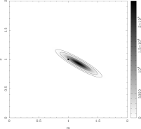
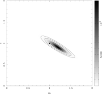
Figure 1: Left: the two data sets ${\textbf{{D}}}_{1}$ (solid circles) and ${\textbf{{D}}}_{2}$ (open squares) drawn from the straight line model with slope $m=1$ and intercept $c=1$ (solid line), and subject to independent Gaussian noise of rms $\sigma_{1}=0.1$ and $\sigma_{2}=0.1$ respectively. Middle: the (unnormalised) posterior $\overline{\Pr}(\mn@boldsymbol{\theta}|{\textbf{{D}}},H_{0})$ corresponding to the standard approach to parameter estimation. Right: the (unnormalised) posterior $\overline{\Pr}(\mn@boldsymbol{\theta}|{\textbf{{D}}},H_{1})$ corresponding to the hyperparameters approach. In each case, the true parameter values are indicated by the solid circle, and the contours contain 68, 95 and 99 per cent respectively of the total probability.

6 A toy problem

To illustrate the potential usefulness of the hyperparameters approach to weighting datasets, in this section we apply the method to the classic parameter estimation problem of fitting a straight line through a set of data points. In particular, we will show how the use of hyperparameters as weights can overcome the common problems of inaccurately quoted error-bars and the presence of systematic errors in the measurements (see also Bridle 2000).

Let us suppose that the true underlying model for some process is the straight line

$$y(x)=mx+c,$$ (49)

where the slope $m=1$ and the intercept $c=1$. We assume that two independent sets of measurements ${\textbf{{D}}}_{1}$ and ${\textbf{{D}}}_{2}$ are made, each of which contains five data points, so $n_{1}=5$ and $n_{2}=5$. In simulating each dataset, the $x$-values are drawn at random from a uniform distribution between zero and unity, and we assume that these values are known precisely. The corresponding $y$-values are independently distributed about their true model values according to a Gaussian distribution of known variance $\sigma_{k}$ for each data set. Thus, the likelihood function for the $k$th dataset has the Gaussian form given by (29) and (30), where $(\mn@boldsymbol{\mu}_{k})_{j}=m({\textbf{{x}}}_{k})_{j}+c$ and ${\textbf{{V}}}_{k}=\mbox{diag}(\sigma_{k}^{2},\ldots,\sigma_{k}^{2})$. Thus, in this simple example, the covariance matrix does not depend on the parameters $m$ and $c$.

We now consider three different scenarios, which illustrate the general useful properties the hyperparameters technique for weighting datasets. We note that, for this simple toy problem, it is clear from a plot of the data points if inconsistencies exist between two datasets, and we will see that the hyperparameters approach verifies our initial suspicions where appropriate. Indeed, this toy model was chosen so that inconsistencies revealed by the hyperparameters method are transparent from a plot of the data. It should be remembered, however, that for realistic cosmological datasets and theoretical models, the situation is usually much more complicated. In this case, one is often unable visually to discern any inconsistencies in the data, but these may nevertheless be deduced by using the hyperparameters technique. This is illustrated in section 7.

   

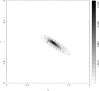
Figure 2: As for Fig. 1, but the reported error-bars on the dataset ${\textbf{{D}}}_{1}$ have been underestimated by a factor of 5.

6.1 Accurate error-bars and no systematic error

In our first case, both data sets ${\textbf{{D}}}_{1}$ and ${\textbf{{D}}}_{2}$ are drawn from the correct model $m=1$ and $c=1$. The noise rms for each dataset is $\sigma_{1}=\sigma_{2}=0.1$, and these (correct) values are used in the parameter estimation process. The two simulated datasets are shown in Fig. 1 (left panel), in which the dataset ${\textbf{{D}}}_{1}$ is denoted by the filled circles, whereas ${\textbf{{D}}}_{2}$ corresponds to the open squares. The true underlying model is plotted as a solid line.

Assuming an appropriately normalised uniform prior on the parameters in the range $m:0\to 2$ and $c:0\to 2$, and using the expressions (31) and (35) for the likelihood in each case, we may calculate the (unnormalised) posteriors $\overline{\Pr}(m,c|{\textbf{{D}}},H_{0})$ and $\overline{\Pr}(m,c|{\textbf{{D}}},H_{1})$ corresponding to the standard and hyperparameters approaches respectively (where D denotes the combination of the datasets ${\textbf{{D}}}_{1}$ and ${\textbf{{D}}}_{2}$). These posterior distributions are plotted in Fig. 1 (middle and right panels), in which the contours contain 68, 95 and 99 per cent respectively of the total probability; the true parameter values are indicated by a solid circle.

In both cases $H_{0}$ and $H_{1}$, the posterior distributions appear very similar and contain the true parameter values at about the 68 per cent confidence level. However, since the prior and the likelihood function in each case are properly normalised, the greyscale units on the plots in Fig. 1 are not arbitrary. Indeed, the evidence in each case can be calculated directly by integrating numerically under these distributions, and we find

$$\frac{\Pr({\textbf{{D}}}|H_{1})}{\Pr({\textbf{{D}}}|H_{0})}=0.54.$$

This indicates that standard approach is very slightly preferred or, equivalently, that the introduction of hyperparameters is marginally disfavoured by the data. An evidence ratio of order unity does not, however, provide a strong indication that one case is preferred over the other. We may conclude that, in this case, our ability to infer the parameter values $m$ and $c$ from the data is essentially unaffected by the introduction of hyperparameters.

It is interesting to compare the exact evidence ratio above with that obtained using the approximate expression (48), in which each posterior distribution is approximated by a Gaussian centred at its peak. Since the function (49) is linear in the parameters $m$ and $c$, and the covariance matrices ${\textbf{{V}}}_{k}$ do not depend on these parameter, the posterior $\overline{\Pr}(\mn@boldsymbol{\theta}|{\textbf{{D}}},H_{0})$ is, in fact, truly Gaussian. We found, in this case, that the approximate expression (10) for the evidence did indeed agree with that obtained by direct numerical integration. In the hyperparameters case, however, the posterior $\overline{\Pr}(\mn@boldsymbol{\theta}|{\textbf{{D}}},H_{1})$ is not Gaussian. Nevertheless, we found that the approximate expression (10) underestimated the true evidence value by only 2 per cent, and the approximate evidence ratio was found to be 0.53.

Finally, we note the effective weight assigned to each dataset at the peak $\hat{\mn@boldsymbol{\theta}}_{1}$ of the hyperparameters posterior $\overline{\Pr}(\mn@boldsymbol{\theta}|{\textbf{{D}}},H_{1})$. These values are given by (44) evaluated at this point, and we find $\alpha_{1}^{\rm eff}(\hat{\mn@boldsymbol{\theta}}_{1})=1.79$ and $\alpha_{2}^{\rm eff}(\hat{\mn@boldsymbol{\theta}}_{1})=2.64$.

6.2 Inaccurate error-bars and no systematic error

In this case, the datasets ${\textbf{{D}}}_{1}$ and ${\textbf{{D}}}_{2}$ are identical to those used in the previous subsection, but we assume that the quoted errors-bars on the dataset ${\textbf{{D}}}_{1}$ have been underestimated by a factor of 5, while the error-bars on the dataset ${\textbf{{D}}}_{2}$ are quoted correctly. Thus, in the parameter estimation procedure, we assume the (incorrect) values $\sigma_{1}=0.02$ and $\sigma_{2}=0.1$. The data points and their reported error-bars are shown in Fig. 2 (left panel).

The resulting (unnormalised) posteriors $\overline{\Pr}(\mn@boldsymbol{\theta}|{\textbf{{D}}},H_{0})$ and $\overline{\Pr}(\mn@boldsymbol{\theta}|{\textbf{{D}}},H_{1})$ are shown in the middle and right-hand panels of the figure. In this case, the two posteriors are very different. In the standard approach $H_{0}$, the posterior distribution is tightly constrained about its maximum as a result of underestimating the errors on dataset ${\textbf{{D}}}_{1}$. Indeed, this posterior is virtually indistinguishable from that calculated from the dataset ${\textbf{{D}}}_{1}$ alone. The true parameter values are excluded at a confidence level that far exceeds the 99 per cent limit. In the hyperparameters case, however, the posterior is much broader and resembles the corresponding distribution in Fig. 1. In particular, the true parameter values are comfortably contained within the 95 per cent confidence limit.

Integrating under the posterior distributions directly, the exact evidence ratio is found to be

$$\frac{\Pr({\textbf{{D}}}|H_{1})}{\Pr({\textbf{{D}}}|H_{0})}=2.1\times 10^{4},$$

which clearly implies that the data favour the introduction of hyperparameter weights. Using the expression (48), the approximate evidence ratio is $1.6\times 10^{4}$, which shows that the Gaussian approximation to the hyperparameters posterior is once again reasonably accurate.

At the peak $\hat{\mn@boldsymbol{\theta}}_{1}$ of the hyperparameters posterior, we find the effective weights assigned to the two datasets ${\textbf{{D}}}_{1}$ and ${\textbf{{D}}}_{2}$ to be $\alpha_{1}^{\rm eff}(\hat{\mn@boldsymbol{\theta}}_{1})=0.12$ and $\alpha_{2}^{\rm eff}(\hat{\mn@boldsymbol{\theta}}_{1})=1.28$. Thus, the first dataset (with error-bars underestimated by a factor of 5) has been assigned an appropriate smaller statistical weight.

6.3 Accurate error-bars and a systematic error

   

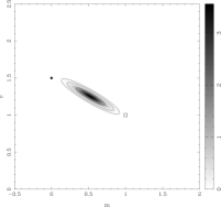
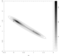
Figure 3: Left: the dataset ${\textbf{{D}}}_{1}$ (solid circles) drawn from the straight-line model with slope $m=0$ and intercept $c=1.5$ (dashed line) and the dataset ${\textbf{{D}}}_{2}$ (open squares) drawn from the straight-line model with slope $m=1$ and intercept $c=1$ (solid line); each dataset is subject to independent Gaussian noise of rms $\sigma_{1}=0.1$ and $\sigma_{2}=0.1$ respectively. Middle: the (unnormalised) posterior $\overline{\Pr}(\mn@boldsymbol{\theta}|{\textbf{{D}}},H_{0})$ corresponding to the standard approach to parameter estimation. Right: the (unnormalised) posterior $\overline{\Pr}(\mn@boldsymbol{\theta}|{\textbf{{D}}},H_{1})$ corresponding to the hyperparameters approach. In each case, the true parameter values for dataset ${\textbf{{D}}}_{1}$ are indicated by the solid circle and the true parameter values for dataset ${\textbf{{D}}}_{2}$ are indicated by an open square. The contours in each case contain 68, 95 and 99 per cent respectively of the total probability.

   

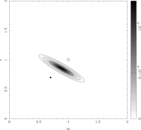
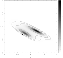
Figure 4: As for Fig. 3, except that the dataset ${\textbf{{D}}}_{1}$ (solid circles) is drawn from the straight-line model with slope $m=0.7$ and intercept $c=0.7$.

We now consider the introduction of a systematic error into the dataset ${\textbf{{D}}}_{1}$. This is simulated by drawing this dataset from an incorrect straight-line model, for which the parameter values $m$ and $c$ differ from unity. Dataset ${\textbf{{D}}}_{2}$, however, is still drawn from the correct straight-line model with $m=1$ and $c=1$. We shall, in fact, consider two separate complementary cases. In the first case, we introduce a systematic error in the direction of the natural degeneracy line in the $(m,c)$-plane, whereas, in the second case, the introduced systematic error is orthogonal to the natural degeneracy line. In both cases, we assume that the error-bars on each dataset are quoted accurately as $\sigma_{1}=0.1$ and $\sigma_{2}=0.1$ respectively.

6.3.1 Case 1

In our first case, dataset ${\textbf{{D}}}_{1}$ is drawn from a straight line with slope $m=0$ and intercept $c=1.5$. The datasets ${\textbf{{D}}}_{1}$ and ${\textbf{{D}}}_{2}$ are shown in Fig. 3 (left panel), together with the underlying straight-line models from which each is drawn. The resulting posterior distributions $\overline{\Pr}(\mn@boldsymbol{\theta}|{\textbf{{D}}},H_{0})$ and $\overline{\Pr}(\mn@boldsymbol{\theta}|{\textbf{{D}}},H_{1})$ are shown in the middle and right-hand panels of the figure. Once again, the two posteriors are very different. In the standard approach, $H_{0}$, the posterior distribution peaks between the two sets of true values. In spite of the fact that the two sets of parameter values define a direction along the natural degeneracy line in the $(m,c)$-plane, neither is contained within the 99 per cent confidence contour, and so both models are excluded at a high significance level. In the hyperparameters case, however, the posterior is much further extended along the natural degeneracy line. In particular, we note that the distribution is bimodal, with each peak lying close to one of the true sets of parameter values. Thus, the hyperparameters indicates the presence of two underlying models for the data, which signals an inconsistency between the two datasets. This could be interpreted as one (or both) of the datasets containing a systematic error.

The exact evidence ratio in this case is found to be

$$\frac{\Pr({\textbf{{D}}}|H_{1})}{\Pr({\textbf{{D}}}|H_{0})}=11.6,$$

which gives a reasonably robust indication that the data favour the introduction of hyperparameters. Using the expression (48), the approximate evidence ratio is given by 4.8. The reason for the large inaccuracy in this case is that the Gaussian approximation to the bimodal hyperparameters posterior is clearly rather poor. In fact, as might be expected in this case, the Gaussian approximation underestimates the true value of the evidence by about a factor of two.

Although the hyperparameters posterior is bimodal, the global maximum $\hat{\mn@boldsymbol{\theta}}_{1}$ occurs at the peak close to the parameter values from which the dataset ${\textbf{{D}}}_{1}$ was drawn. At this peak, we find the effective weights assigned to the two datasets ${\textbf{{D}}}_{1}$ and ${\textbf{{D}}}_{2}$ are $\alpha_{1}^{\rm eff}(\hat{\mn@boldsymbol{\theta}}_{1})=3.11$ and $\alpha_{2}^{\rm eff}(\hat{\mn@boldsymbol{\theta}}_{1})=0.18$, which indicates (correctly) that the first dataset has been assigned a larger statistical weight at this point in parameter space. However, at the subsidiary peak $\hat{\mn@boldsymbol{\theta}}^{\prime}_{1}$ located near the parameter values from which the dataset ${\textbf{{D}}}_{2}$ was drawn, we find $\alpha_{1}^{\rm eff}(\hat{\mn@boldsymbol{\theta}}^{\prime}_{1})=0.11$ and $\alpha_{2}^{\rm eff}(\hat{\mn@boldsymbol{\theta}}_{1})=6.41$, and so the roles of the datasets have been reversed.

6.3.2 Case 2

In our second case, dataset ${\textbf{{D}}}_{1}$ is drawn from a straight line with slope $m=0.7$ and intercept $c=0.7$. The datasets ${\textbf{{D}}}_{1}$ and ${\textbf{{D}}}_{2}$ are shown in Fig. 4 (left panel), together with the underlying straight-line models from which each is drawn. The the middle and right-hand panels of the figure show the resulting posterior distributions $\overline{\Pr}(\mn@boldsymbol{\theta}|{\textbf{{D}}},H_{0})$ and $\overline{\Pr}(\mn@boldsymbol{\theta}|{\textbf{{D}}},H_{1})$. As in Case 1, the standard approach produces a posterior distribution that peaks between the two true sets of parameters values, excluding both at a high significance level. We note, in this case, that the two sets of true parameter values define a direction orthogonal to the natural degeneracy line in the $(m,c)$-plane. In the hyperparameters case, however, the posterior is again bimodal, with each peak lying close to one of the true sets of parameter values. Thus, once again the hyperparameters approach signals the presence of two underlying models for the data and hence an inconsistency between the datasets.

The exact evidence ratio is found to be

$$\frac{\Pr({\textbf{{D}}}|H_{1})}{\Pr({\textbf{{D}}}|H_{0})}=5.9\times 10^{3},$$

which strongly implies that the data favour the introduction of hyperparameters. In this case, the approximate evidence ratio (48) is given by $2.4\times 10^{3}$. As in Case 1, the Gaussian approximation underestimates the true value of the evidence for the hyperparameters posterior by about a factor of 2, as a result of it being bimodal.

Once again the effective weights clearly show which dataset is dominating at each peak of the hyperparameters posterior. At the global maximum $\hat{\mn@boldsymbol{\theta}}_{1}$, we find $\alpha_{1}^{\rm eff}(\hat{\mn@boldsymbol{\theta}}_{1})=0.066$ and $\alpha_{2}^{\rm eff}(\hat{\mn@boldsymbol{\theta}}_{1})=7.96$, whereas at the subsidiary maximum $\hat{\mn@boldsymbol{\theta}}^{\prime}_{1}$ we obtain $\alpha_{1}^{\rm eff}(\hat{\mn@boldsymbol{\theta}}^{\prime}_{1})=3.31$ and $\alpha_{2}^{\rm eff}(\hat{\mn@boldsymbol{\theta}}_{1})=0.079$.

7 A cosmological illustration

In this section, we illustrate the hyperparameters technique for weighting datasets by applying it to recent measurements of the CMB power spectrum provided by the BOOMERANG (Netterfield et al. 2001), MAXIMA (Lee et al. 2001) and DASI (Halverson et al. 2001) experiments. We also include the 8 data points for large-scale normalisation of the spectrum provided by the COBE satellite. The flat band-powers reported by each of these experiments are plotted in Fig 5.

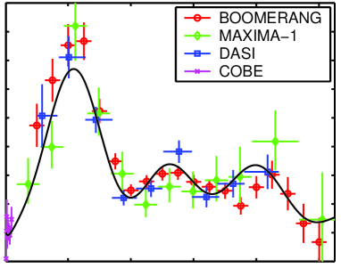
Figure 5: The flat-band power estimates of the CMB power spectrum reported by the COBE, BOOMERANG, MAXIMA, DASI experiments. The solid line corresponds to the CMB power spectrum for a spatially-flat inflationary CDM model with no tensor contribution and $\Omega_{m}=0.3$, $\Omega_{b}h^{2}=0.02$, $h=0.7$, $n=1$, $\tau=0$ and $Q=18$ $\mu$K.

The solid line in the plot corresponds to the predicted CMB power spectrum for a spatially-flat inflationary CDM model with no tensor contribution and $\Omega_{m}=0.3$, $\Omega_{b}h^{2}=0.02$, $h=0.7$, $n=1$, $\tau=0$ and $Q=18$ $\mu$K.

From Fig. 5, we see immediately that there is good agreement between the datasets, all of which are broadly consistent with the plotted theoretical CMB power spectrum. One would therefore expect the inclusion of and marginalisation over hyperparameter weights not to be warranted by the data. It should also be remembered, however, that the points and error-bars plotted in the figure do not include the calibration and beam uncertainties associated with each experiment. Indeed, since these uncertainties can be as large as 20 per cent in some cases, one would naively expect the envelope of the experimental data to be much wider, resulting in poorer agreement with the theoretical spectrum. As we will see below, this naive observation is supported by the proper calculation of Bayesian evidences.

7.1 No calibration or beam uncertainty

We first analyse the data without including calibration and beam errors, i.e. as plotted in Fig. 5. For each dataset ${\textbf{{D}}}_{k}$ $(k=1,2,3,4)$, we assume the uncertainties on the flat band-powers are described by a multivariate Gaussian of the form given in (29). For the COBE and DASI datasets, we use the publicly-available window functions and full covariance matrix ${\textbf{{V}}}_{k}$ for each dataset. In the absence of the equivalent information for the BOOMERANG and MAXIMA experiments, we assume a top-hat window function for the spectrum in each bin and neglect correlations between bins. This approach is a good approximation of the correct one (see de Bernardis et al. 2001) and does not affect our conclusions.

Denoting the totality of the resulting data by the vector D, the next step in the analysis is to calculate the unnormalised posterior distributions $\overline{\Pr}(\mn@boldsymbol{\theta}|{\textbf{{D}}},H_{0})$ and $\overline{\Pr}(\mn@boldsymbol{\theta}|{\textbf{{D}}},H_{1})$, corresponding to the standard and hyperparameters approaches respectively, for some set of cosmological parameters $\mn@boldsymbol{\theta}$. For the purposes of illustration, we assume a spatially-flat Universe ($\Omega_{k}=1$), with no tensor contribution to the CMB spectrum, and take the parameter vector $\mn@boldsymbol{\theta}$ to consist of 5 parameters, namely the normalisation $Q$, the Hubble parameter $h$, the matter density $\Omega_{\rm m}$, the physical baryon density $\Omega_{\rm b}h^{2}$ and the scalar spectral index $n$. Since the parameter space is only 5-dimensional, it is feasible to evaluate the unnormalised posteriors over a hypercube. Thus, we assume (suitably normalised) uniform priors on the parameters, with the ranges $12<Q<24$ $\mu$K, $0.5<h<0.9$, $0.1<\Omega_{\rm m}<0.5$, $0.01<\Omega_{\rm b}h^{2}<0.04$ and $0.8<n<1.2$. The corresponding likelihood functions for the hypotheses $H_{0}$ and $H_{1}$ have the forms (31) and (35) respectively. The posterior distribution is calculated at 20 points in the directions $Q$, $h$ and $\Omega_{m}$ in parameter space, and at 10 points in the directions $n$ and $\Omega_{b}h^{2}$. The theoretical power spectrum corresponding to each model was calculated using CAMB (Lewis, Challinor & Lasenby 2000).

    

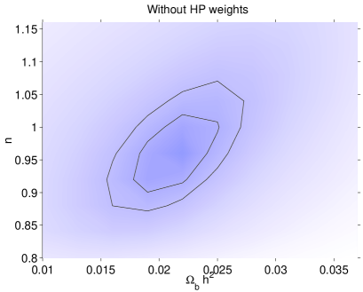
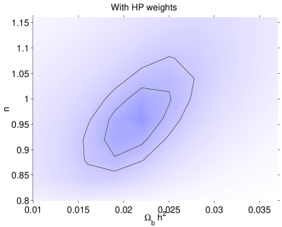
Figure 6: The standard posterior $\overline{\Pr}(n,\Omega_{b}h^{2}|{\textbf{{D}}},H_{0})$ (left) and the hyperparameters posterior $\overline{\Pr}(n,\Omega_{b}h^{2}|{\textbf{{D}}},H_{1})$ (right) obtained by marginalisation over the parameters $Q$, $h$ and $\Omega_{m}$, assuming no calibration or beam uncertainties in the data plotted in Fig. 5.

Since $\overline{\Pr}(\mn@boldsymbol{\theta}|{\textbf{{D}}},H_{0})$ and $\overline{\Pr}(\mn@boldsymbol{\theta}|{\textbf{{D}}},H_{1})$ are each calculated over a hypercube in the 5-dimensional parameter space, one can calculated the evidence integrals (36) and (37) directly, and one finds the exact evidence ratio to be

$$\frac{\Pr({\textbf{{D}}}|H_{1})}{\Pr({\textbf{{D}}}|H_{0})}=0.05.$$

This indicates that the data do not support the inclusion of and subsequent marginalisation over a free hyperparameter weight $\alpha_{k}$ $(k=1,2,3,4)$ for each dataset. In other words, as expected, the datasets are statistically consistent both with one another and with the range of theoretical models with which they have been compared.

For illustration, let us consider the constraints placed by the current CMB data on the parameters $n$ and $\Omega_{b}h^{2}$ with and without the inclusion of hyperparameter weights. The limits placed on these parameters by the standard and hyperparameters approaches respectively are easily obtained by marginalising the corresponding posteriors $\overline{\Pr}(\mn@boldsymbol{\theta}|{\textbf{{D}}},H_{0})$ and $\overline{\Pr}(\mn@boldsymbol{\theta}|{\textbf{{D}}},H_{1})$ over the remaining parameters $Q$, $h$ and $\Omega_{m}$. The resulting distributions are shown in Fig. 6, together with corresponding the 68 and 95 per cent confidence contours. Although the above evidence ratio shows that the data do not favour marginalisation over hyperparameter weights, we see that their inclusion does not significantly affect the constraints placed on the parameters. This illustrates that, for statistically consistent datasets, the standard and hyperparameters techniques may be use interchangeable without degrading the constraints on cosmological parameters. In particular, we note that the current CMB data are consistent with the scale invariant spectrum $n=1$ and the nucleosynthesis constraints on $\Omega_{b}h^{2}$. Indeed, by performing an additional marginalisation over $n$ or $\Omega_{b}h^{2}$ we obtain (to two significant figures) the one-dimensional 68-per cent confidence intervals $0.019<\Omega_{b}h^{2}<0.023$ and $0.92<n<1.00$ for both the case $H_{0}$ and $H_{1}$.

7.2 Marginalisation over calibration and beam uncertainties

So far our analysis has ignored the calibration and beam uncertainties associated with each dataset. Any meaningful analysis of these data must, however, include these effects of these ‘nuisance’ parameters. As with hyperparameter weights, the correct approach is to assign some prior to these parameters and then marginalise over them. For calibration and beam uncertainties, one does have a priori knowledge of both the expectation value of each parameter and the range of values it might take (i.e. its variance). Thus, as shown in section 4.1, it is appropriate to adopt independent Gaussian priors on the calibration and beam uncertainties. As discussed in detail by Bridle et al. (2001), for Gaussian likelihood functions of the form (29), one can again perform this marginalisation analytically. Moreover, the resulting likelihood function after marginalisation is also of the form (29), but with a modified covariance matrix ${\textbf{{V}}}^{\prime}_{k}$.

Using these modified datasets, one can then calculate the posteriors $\overline{\Pr}(\mn@boldsymbol{\theta}|{\textbf{{D}}},H_{0})$ and $\overline{\Pr}(\mn@boldsymbol{\theta}|{\textbf{{D}}},H_{1})$ over the same hypercube in the 5-dimensional parameter space as used above, and evaluate the evidence integrals (36) and (37) directly. In this case, the evidence ratio is found to be

$$\frac{\Pr({\textbf{{D}}}|H_{1})}{\Pr({\textbf{{D}}}|H_{0})}=0.08,$$

which illustrates that the inclusion of and marginalisation over hyperparameter weights is once more unwarranted. The corresponding marginalised posteriors in the $(n,\Omega_{b}h^{2})$-plane, with and without marginalisation over are again almost identical and closely resemble those plotted in Fig. 6. One obtains the one-dimensional 68-per cent confidence intervals $0.018<\Omega_{b}h^{2}<0.024$ and $0.90<n<0.99$ for the case $H_{0}$ (without hyperparameter weights) and $0.018<\Omega_{b}h^{2}<0.024$ and $0.90<n<1.00$ for the case $H_{1}$ (with hyperparameter weights). Once again, we see that the inclusion of and marginalisation over hyperparameter weights has little effect on the parameter constraints imposed by the data.

7.3 Evidence for calibration and beam uncertainties

Although the evidence ratios given above show that the current CMB power spectrum data clearly do not require the use of hyperparameter weights in their analysis, it is also interesting to compare the relative evidence values for the cases with and without marginalisation over calibration and beam uncertainties (for both $H_{0}$ and $H_{1}$). The evidence values corresponding to each of the 4 cases we have considered are given in Table 1, where they have been rescaled so that the evidence is unity for the case where no hyperparameter weights are introduced and no marginalisation over calibration and beam uncertainties is performed. We see that the largest evidence value is obtained for the case in which no marginalisation is performed over hyperparameter weights or calibration and beam uncertainties. While one might expect from the data plot in Fig. 5 that the introduction of and marginalisation over hyperparameter weights might not be favoured, it is surprising that the marginalisation over the calibration and beam uncertainties also reduces the evidence for the data. This means that, when compared with the range theoretical models discussed above, the probabilty of obtaining the observed data is highest if one assumes no uncertainty exists in the calibration and beam properties adopted by each experiment, rather than marginalising over the reported uncertainties in these parameters. Thus we see that the evaluation of evidences has provided quantitative support for our earlier naive observation that the CMB datasets plotted in Fig. 5 agree remarkably well given the 5–20 per cent calibration uncertainties alone (which are not plotted). We note here simply that this eventuality is unlikely to occur by chance.

	No HP weights	With HP weights
No cal/beam marginalisation	$1.0$	$5\times 10^{-2}$
With cal/beam marginalisation	$4\times 10^{-4}$	$3\times 10^{-5}$

Table 1: The relative Bayesian evidences for the obtaining the current CMB power spectrum data in the 4 cases discussed in the text.

8 Conclusions

We have presented a general account of the use of hyperparameters in the analysis of cosmological datasets. In particular, we have concentrated on applying the hyperparameters technique to the problem of weighting different datasets in a joint analysis aimed at estimating some set of cosmological parameters. The basic approach is to assign a free hyperparameter weight to each dataset and then perform a marginalisation over these hyperparameters. This method allows the statistical properties of the data themselves to determine the effective weight given to each dataset and is in sharp contrast to the more common practice of excluding certain datasets from the analysis, which hence are assigned a weight of zero, and analysing the remaining datasets with equal weights.

Assuming the expected value of the hyperparameter weight on each dataset to be unity, we find that the prior on each hyperparameter should be of exponential form, rather than the more commonly used improper Jeffrey’s prior. In either case, the marginalisation over the hyperparameters may be performed analytically for Gaussian likelihood functions. Since the exponential prior is properly normalised, in this case one may also calculate the Bayesian evidence for the data given the hyperparameters model. This evidence value can then be compared with the corresponding evidence for the data in the absence of hyperparameters, in order to determine whether the data warrant the inclusion of hyperparameters in the first instance. In each case, the evidence may be calculated either by direct integration, for low-dimensionality parameter spaces, or approximated straightforwardly by assuming each posterior to be Gaussian near its peak.

The hyperparameter approach to weighting datasets is illustrated by applying it to the classic toy model of fitting a straight to a number of datasets. We find the hyperparameters technique correctly infers the existence of systematic errors and/or misquoted random errors in the datasets. In such cases, the evidence ratio for the hyperparameters and standard approaches clearly indicates that the data warrant the introduction of the hyperparameters. Nevertheless, in the case where no systematic errors exists, and the random errors are accurately quoted, the evidence ratio correctly indicates that hyperparameters should not be included in the analysis.

Finally, the hyperparameters technique is applied to the latest measurements of the cosmic microwave background (CMB) power spectrum by the BOOMERANG, MAXIMA and DASI experiments, together with the large-scale normalisation of the power spectrum provided by the COBE satellite. The evidence ratio between the hyperparameters and standard approach shows that the current CMB datasets do not warrant the inclusion of hyperparameters weights and a subsequent marginalisation over them. In other words, the datasets are statistically consistent both with one another and with the range of theoretical models with which they were compared. Nevertheless, the inclusion of hyperparameters in shown not to lessen the constraints imposed by the data on cosmological parameters.

The analysis is repeated for the case in which one first marginalises over the beam and calibration uncertainties associated with each dataset, and again the evidence ratio shows that the inclusion of hyperparameter weights is unwarranted. Of more interest is the comparison of evidences with and without marginalisation over calibration and beam uncertainties. This shows that the evidence for the data is largest if one assumes no uncertainty in the calibration and beam properties, but instead adopt the values corresponding to those implied by the published CMB power spectrum points for each dataset. This is unlikely to occur by chance.

ACKNOWLEDGMENTS

MPH thanks Steve Gull and Anthony Lasenby for some illuminating discussions concerning Bayes’ theorem and probability theory. The authors also thank Antony Lewis for providing the $C_{\ell}$-grid and Anze Slozar for the use of his $C_{\ell}$-grid interpolation routines. SLB acknowledges Selwyn College, Cambridge, for support in the form of the Trevelyan Research Fellowship.

References

- [] Bishop C.M., 1995, Neural Networks for Pattern Recognition, Oxford University Press, Oxford
- [] Bridle S.L., 2000, Ph.D. Thesis, University of Cambridge.
- [] Bridle S.L., Crittenden R., Melchiorri A., Hobson M.P., Kneissl R., Lasenby A.N., 2002, MNRAS, in press (astro-ph/0112114)
- [] Bond J.R., Jaffe A., Knox L., 2000, ApJ, 533, 19
- [] de Bernardis P. et al., 2001, ApJ, in press (astro-ph/0105296)
- [] Erdogdu P, Ettori S., Lahav O., 2002, MNRAS, submitted (astro-ph/0202357)
- [] Godwin P., Lynden-Bell D., 1987, MNRAS, 229, 7
- [] Halverson et al., 2001, ApJ, submitted (astro-ph/0104489)
- [] Jaffe A., 1996, ApJ, 471, 24
- [] Jaynes E.T., 1957a, Phys. Rev., 106, 620
- [] Jaynes E.T., 1957b, Phys. Rev., 108, 171
- [] John M.V., Narlikar J.V., 2002, Phys. Rev. D, in press (astro-ph/0111122)
- [] Knox L., Christensen N., Skordis C., 2001, ApJL, submitted (astro-ph/0109232)
- [] Lahav O., Bridle S.L., Hobson M.P., Lasenby A.N., Sodré L., Jr., 2000, MNRAS, 315, L45 (Paper I)
- [] Lee et al., 2001, ApJ, 561, L1
- [] Lewis A., Challinor A., Lasenby A., 2000, ApJ, 538, 473
- [] Netterfield C.B. et al., 2001, ApJ, submitted (astro-ph/0104460)
- [] Press W.H., 1996, in Unsolved Problems in Astrophysics, Proc. Conference in Honour of John Bahcall, ed. J.P. Ostriker. Princeton University Press
- [] Shannon C.E., 1948, Bell Sys. Tech. J., 27, 379
- [] Sivia D.S., 1996, Data Analysis: A Bayesian Tutorial. Oxford University Press