The EXPLORE Project I: A Deep Search for Transiting Extrasolar Planets

Abstract

Planet transit searches promise to be the next breakthrough for extrasolar planet detection, and will bring the characterization of short-period planets into a new era. Every transiting planet discovered will have a measured radius, which will provide constraints on planet composition, evolution, and migration history. Together with radial velocity measurements, the absolute mass of every transiting planet will be determined.

In this paper we discuss the design considerations of the EXPLORE (EXtrasolar PLanet Occultation REsearch) project, a series of transiting planet searches using 4-m-class telescopes to continuously monitor a single field of stars in the Galactic Plane in each $\sim 2$ week observing campaign. We discuss the general factors which determine the efficiency and the number of planets found by a transit search, including time sampling strategy and field selection. The primary goal is to select the most promising planet candidates for radial velocity follow-up observations. We show that with very high photometric precision light curves that have frequent time sampling and at least two detected transits, it is possible to uniquely solve for the main parameters of the eclipsing system (including planet radius) based on several important assumptions about the central star. Together with a measured spectral type for the star, this unique solution for orbital parameters provides a powerful method for ruling out most contaminants to transiting planet candidates. For the EXPLORE project, radial velocity follow-up observations for companion mass determination of the best candidates are done on 8-m-class telescopes within two or three months of the photometric campaigns. This same-season follow-up is made possible by the use of efficient pipelines to produce high quality light curves within weeks of the observations. We conclude by presenting early results from our first search, EXPLORE I, in which we reached $<1$% rms photometric precision (measured over a full night) on $\sim$37,000 stars with $14.5\leq I\leq 18.2$.

1 Introduction

The discovery of giant extrasolar planets in the mid-1990s using radial velocity techniques (e.g., Marcy, Cochran, & Mayor 2000) heralded a new era in the study of planetary systems, and to date $\sim$80 extrasolar giant planets have been discovered. Radial velocity searches produced the completely unexpected discovery of massive planets in few-day period orbits, such as 51 Peg b (Mayor & Queloz 1995). To date 17 systems with orbital distances of $<$0.1 AU and periods of a few days have been found¹⁰. The existence of a class of close-in giant planets shows that planetary systems can be radically different from our own. The discovery of close-in giant planets sparked much theoretical work on planet formation and migration scenarios to explain the proximity of giant planets to the parent star, such as: planetesimal scattering (e.g., Murray et al. 1998), planet-disk or binary star interactions (e.g., Lin, Bodenheimer, & Richardson 1996; Holman, Touma, & Tremaine 1997), and dynamical instabilities in multiple giant planet systems (Rasio & Ford 1996).

The existence of a significant population of close-in extrasolar giant planets (CEGPs) makes the method of finding planetary systems via transits of their parent star very promising; the probability that a given planet will show transits is inversely proportional to its orbital distance, and relatively large for CEGPs around main-sequence stars ($\sim$10%). Moreover, for planets with periods of 3–4 days, it is possible to detect two or more transits via high photometric precision light curves that span a relatively small number of nights. A photometric precision of 1%, which can be routinely achieved with CCD cameras, is sufficient to detect giant planets around sun-like stars (see Figure 1). The advent of wide-field CCD mosaic cameras greatly increases the efficiency of the transit search method, since a very large number of stars can be monitored at once.

The principal motivation for the transit search method is the possibility of characterizing planets in a way not possible with current radial velocity surveys: radius. Transiting planets are currently the only ones whose radii can be determined (based on transit depth and stellar radius). The planet radius can be measured to better than 10% precision with follow-up ultra-high precision photomtery on transiting planets (e.g., Brown et al. 2001; Cody & Sasselov 2002). A radius measurement is necessary to constrain the planet evolution and migration history and also provides constraints on planet composition and atmosphere through evolutionary models. The radii of CEGPs are especially interesting for planetary physics due to the evolution of the planet in proximity to the central star and because of the as yet unknown migration timescales. Very interesting recent work (Guillot & Showman 2002) has shown that the observed radius of transiting planet HD209458b (Brown et al. 2001) disagrees with the theoretically predicted radius by 30% for their preferred evolutionary models. This implies there are atmospheric or interior physical processes taking place which are not currently known. The determination of planet radius as a function of stellar type and in different stellar environments will be a major step forward in planetary characterization and in understanding giant planet physics.

Follow-up observations of planets found from transit surveys can be very important for planet confirmation and characterization. Radial-velocity planet mass measurements are required in order to confirm transit candidates as actual planets. Mass measurements for transiting planets are facilitated by the fact that the phase and period for the system are known in advance, and therefore it is possible to conduct observations at times of maximum radial velocity amplitude. For faint stars (V$\sim 18$) it is currently possible to measure masses or place upper limits as low as a couple of $M_{J}$ (e.g., Mallén-Ornelas et al. 2002). Brown et al. (2001) give a list of interesting follow-up studies possible for transiting planets around bright stars. For fainter stars large planetary moons could be detected from transit timing. More importantly, transit searches have the possibility of probing new regions of parameter space compared to current radial velocity planet searches. For example, fainter stars can be monitored in a photometric planet transit search, allowing planets to be found in more distant environments and orbiting intrinsically smaller stars. Transit searches are unbiased with respect to unusual spectral characteristics, which may lead to unexpected discoveries and help constrain planet formation models.

One confirmed transiting extrasolar planet, HD 209458 b, is currently known (Charbonneau et al. 2000; Henry et al. 2000). HD 209458 b was discovered by the radial velocity technique, and follow-up photometry determined that it transits its parent star. More than twenty groups around the world are currently using photometry to search for transiting extrasolar planets. Many different environments are being or have been searched, including the globular cluster 47 Tuc (Gilliland et al. 2000), open clusters of different metallicities (Howell et al. 1999; Mochejska et al. 2002; Quirrenbach et al. 2001; Street et al. 2001, 2002; Burke et al. 2002), field stars with magnitude $\lesssim 13$ (Borucki et al. 2001; Brown & Charbonneau 2001), and $13\lesssim I\lesssim 17.75$ stars in the direction of the Galactic center (Udalski et al. 2002a,b). There have also been several conceptual papers about where and how to look for transits, including early papers by Struve (1952), Rosenblatt (1971), and Borucki & Summers (1984), a thorough and prescient paper by Giampapa, Craine, & Hott (1995), and later papers after the discovery of CEGPs, including cluster search strategies (Janes 1996) and searches towards the Galactic Bulge with 10-m-class telescopes (Gaudi 2000).

Although no planets found from a transit search have yet been confirmed with a mass detection from radial velocity follow-up, many planet candidates now exist and are being followed-up for mass confirmation. Notably, the OGLE-III search (Udalski et al. 2002a,b) has made public a list of over 50 stars with small transiting companions, available to the astronomical community for follow-up. The Vulcan project (Borucki et al. 2001; Jenkins, Caldwell & Borucki 2002) and the EXPLORE project (this paper; Mallén-Ornelas et al. 2002) have also produced planet candidates which are being followed-up with radial velocity observations. Although it is disappointing that the transit search method has not yet resulted in any confirmed planets, a steep learning curve as well as some lead-up time is expected for this kind of enterprise. It is not clear how much of the current low planet yield results from the nature of the problem (e.g., due to an intrinsically low frequency of close-in planets in the types of stars surveyed so far), and how much from technical challenges faced by different transit surveys. One of the limiting factors so far is that many transit surveys have not monitored enough stars with sufficiently high photometric precision. This paper has the goal of outlining the necessary steps for a successful transit search with a CCD mosaic camera on a 2–4m telescope, and in addition describes the main false positives that can be ruled out with high-precision, high time sampling photometry and spectral typing of stars.

This paper presents a framework for the design of a search for transiting planets around field stars and presents early results from the EXPLORE (EXtrasolar PLanet Occultation REsearch) project. The EXPLORE project is a set of transit searches using wide-field mosaic cameras on 4-meter-class telescopes with follow-up radial velocity measurements on 8-meter-class telescopes. We start in §2 by describing a very useful property of a high quality light curve with two or more flat-bottomed transits: there is a unique solution for planet and stellar parameters as long as certain important conditions are met. This unique solution can be used to obtain a clean set of planet transit candidates and hence is one of the main motivations for our experimental design. When designing a transit survey it is important to consider the frequency of transiting planets and the transiting planet detection probability. Section 3 presents a description of the factors that affect the number of planets detected and an estimate for the number of planets expected in a transit survey. The issues considered in §3 are of a general nature and can be applied to the design of any planet transit search. When designing a specific planet transit search, a number of interrelated choices must be made in the observational design; in §4, we continue the discussion of survey design by describing the specific aspects of the EXPLORE project strategy. In §5 we present early results from the first search in our project, the EXPLORE I search, conducted in June 2001 at the CTIO 4-m telescope. We summarize and conclude in §6.

2 The Unique Solution of a Two-transit Light Curve

One of the most attractive aspects of transit searches is that much can be learned about a system with an orbiting companion from a good light curve showing two or more eclipses. Here we describe for the first time that a light curve with two or more flat-bottomed eclipses can in principle be used to derive a unique solution of orbital parameters and companion radius, given certain conditions. The unique solution provides a powerful method to select the best planet candidates to be followed up for mass determination. Specifically, the stellar mass $M_{*}$, stellar radius $R_{*}$, companion radius $R_{p}$, orbital distance $D$, and orbital inclination $i$ can be uniquely derived from a light curve with two or more eclipses if the following conditions are met:
$\bullet$ The light curve has an extremely high photometric precision and high time sampling;
$\bullet$ The eclipses have flat bottoms (in a bandpass where limb darkening is negligible), which implies that the companion is fully superimposed on the central star’s disk;
$\bullet$ There are no secondary eclipses (i.e., the brightness of the companion is negligible compared to the central star);
$\bullet$ The period can be derived from the light curve (e.g., the two observed eclipses are consecutive);
$\bullet$ The light comes from a single star, rather than from two or more blended stars;
$\bullet$ The central star is on the main sequence;
$\bullet$ The mass of the companion is negligible compared to that of the central star ($M_{p}\ll M_{*}$);
$\bullet$ The orbit is circular (expected for CEGPs due to their short tidal circularization timescales).

If the above conditions are met, the five parameters $M_{*},R_{*},R_{p},D,$ and $i$ can be uniquely derived from the five equations below. For simplicity, the equations presented here assume that $R_{*}\ll D$. The five equations are:

the transit depth

$$\Delta F=\left(\frac{{R_{p}}}{{R_{*}}}\right)^{2};$$ (1)

the relation between the inclination of the orbit and the shape of the transit light curve, as parametrized by the ratio of the duration of the transit’s flat bottom $t_{flat}$ to the total transit duration $t_{T}$

$$\left(\frac{t_{flat}}{t_{T}}\right)^{2}=\frac{\left(1-\frac{R_{p}}{R_{*}}\right)^{2}-\left(\frac{D}{R_{*}}\cos i\right)^{2}}{\left(1+\frac{R_{p}}{R_{*}}\right)^{2}-\left(\frac{D}{R_{*}}\cos i\right)^{2}};$$ (2)

the total transit duration

$$t_{T}=\frac{PR_{*}}{\pi D}\sqrt{\left(1+\frac{R_{p}}{R_{*}}\right)^{2}-\left(\frac{D}{R_{*}}\cos i\right)^{2}};$$ (3)

Kepler’s Third Law

$$P^{2}=\frac{4\pi^{2}D^{3}}{GM_{*}};$$ (4)

and the mass-radius relation for (sun-like) main sequence stars

$$M_{*}=f(R_{*})\approx R_{*}\frac{M_{\odot}}{R_{\odot}}.$$ (5)

The following observable quantities are measured from the light curve and are used to solve the system of equations: the period $P$, the total transit duration $t_{T}$, the flat eclipse bottom duration $t_{flat}$, and the transit depth $\Delta F$. Determining the five parameters $M_{*},R_{*},R_{p},D,$ and $i$ from the system of equations and observables is a useful shortcut, but in practice the final errors and parameters are directly derived from a fit to the light curve. We note that five model parameters can be extracted from the four observable quantities because of the assumed stellar mass-radius relation (equation (5)), which provides a constraint that does not depend on observations specific to a particular star. Analyzing the error propagation through equations (1) to (5) shows that the most critical inputs are $t_{flat}$, $t_{T}$, and the mass-radius relation. For system parameters similar to those of HD 209458, errors of 10 minutes in $t_{flat}$ or $t_{T}$, or a 20% error in assumed radius at a given mass, leads to errors of about 30% in $M_{*}$ and $\cos i$, and about 15% in $R_{*}$, $R_{p}$, and $D$.

The presence of significant limb darkening will have an effect on the transit depth and shape (see Figure 2). The flat bottom of the transit will become progressively more rounded when viewed at increasingly shorter wavelengths; moreover, a central transit will be deeper than $R_{p}^{2}/R_{*}^{2}$, since a larger fraction of the stellar light is coming from a smaller area of the star. The shape of the transit can still be used to constrain the orbital parameters if an appropriate limb darkening model is adopted. However, given the extra parameters and the uncertainty in the adopted limb darkening model, it is preferable to use light curves taken at long wavelengths so that limb darkening is minimized (Figure 2).

If any of the assumptions listed at the beginning of this section are incorrect for a given light curve, then the derived parameters ($M_{*},R_{*},R_{p},D,$ and $i$) will also be incorrect. If $M_{*}$ and $R_{*}$ can be obtained from spectral classification of the star, then the above system of five equations and unknowns will be overconstrained and can be used to check the correctness of the assumptions about the system. For example, when two transits are separated by an odd number of nights they might not be consecutive transits, since a transit may have occurred during the day at time $P/2$. In general, gaps in time coverage can lead to missed eclipses and the resulting period aliasing. If period aliasing is suspected, the actual period can be determined from the above system of equations plus a spectral type. Even when only one high-quality transit is detected, the three parameters $P$, $R_{p}$, and $i$ can still be constrained from equations (1) through (5) provided the spectral type—and hence $M_{*}$ and $R_{*}$—is known. Another crucial example of the usefulness of obtaining a spectral type is the case of light curve from an unresolved triple system in which two of the stars form an eclipsing binary system. In this case, solving the above equations under the assumption that the light is coming from only one star will generally give a solution for $R_{*}$ and $M_{*}$ that is inconsistent with the spectral type. Thus, by complementing a two-transit light curve with spectra or even broadband colors, much can be learned about an eclipsing system, provided the photometry has very high precision and high time sampling. Further details, error simulations, and applications of the unique solution to a transit light curve are presented in Seager & Mallén-Ornelas (2002).

3 General Considerations for the Design of a Transit Survey

In this section we discuss the factors that should motivate the basic design of any transit survey. The two most important broad considerations for designing a successful survey are: (1) finding planets, and (2) providing useful statistics of planet frequency and characteristics. In broad terms, the number of planets found by a transit search will be determined by:
$\bullet$ frequency of close-in planets around stars in the survey;
$\bullet$ probability of having a geometric alignment that shows transits;
$\bullet$ number of stars surveyed;
$\bullet$ photometric precision;
$\bullet$ window function of the observations.
The last three elements can be controlled by the survey strategy. The following subsections discuss the five factors listed above and their significance for survey strategy.

3.1 Planet Frequency and Detection Probability

An estimate of the fraction of field stars that have transiting short-period planets is useful for designing a transit search. The frequency of transiting planets for a given ensemble of main-sequence stars of similar metallicity, age, and environment can be approximately written as

$$F_{p}=\int\int\int P_{p}(R_{*},R_{p},D)P_{g}(R_{*},D)\hskip 2.84544ptdR_{*}dR_{p}dD.$$ (6)

$P_{p}$ is the probability distribution that a star of radius $R_{*}$ has a planet of radius $R_{p}$ with an orbital distance $D$, and is precisely what a good survey should aim to measure. $P_{p}$ is also likely dependent on stellar metallicity, age, and environment. $P_{p}$ is currently not known because only a small number of CEGPs have been found to date by radial-velocity (RV) planet searches. $P_{g}$ is the geometric probability that a planet will occult its parent star as seen from Earth; $P_{g}\sim R_{*}/D$ for an ensemble of randomly oriented systems with circular orbits and $R_{p}\ll R_{*}\ll D$. A simple estimate of the frequency $F_{p}$ of transiting close-in giant planets ($P\lesssim$4.5  days) can be obtained by assuming all isolated stars have the same frequency of CEGPs as isolated sun-like stars, and adopting $P_{p}\sim 0.007$ (Butler et al. 2001) and the corresponding $P_{g}\sim 0.1$. Assuming that we can detect planets only around isolated stars, and adopting a binary fraction of 1/2, we get $F_{p}=0.00035$. In other words, we expect 1/3000 stars to have a transiting close-in giant planet, with large uncertainty. The uncertainty comes from two sources. First, $P_{p}$ is measured only for nearby isolated sun-like stars with planets of $M_{p}\simeq M_{J}$; moreover this $P_{p}$ estimate comes from surveys that suffer from limited statistics and selection effects which are difficult to characterize. Second, it may be possible to detect transiting planets around a star in a binary system, depending on the brightness ratio of the stars and on the photometric precision.

In practice, the fraction of stars with planets actually discovered by a transit search will likely be much less than $F_{p}\sim 1/3000$. The number of detected planets $N_{p}$ will depend crucially on the window function of the observations $W$, the photometric precision $\delta m$, the time sampling of the observations $\delta t$, and the number of stars monitored $N(R_{*})$. The number of detected planets can be schematically written as

$$N_{p}(W,\delta m)=\int\int\int N(R_{*})P_{p}(R_{*},R_{p},D)P_{g}(R_{*},D)P_{det}(R_{*},R_{p},D,\delta m,\delta t)P_{vis}(W,D,R_{*})\hskip 2.84544ptdR_{*}dR_{p}dD.$$ (7)

Here $P_{det}$ is the probability of detecting a transit of depth $(R_{p}/R_{*})^{2}$ given a photometric precision $\delta m$ and time interval between photometric data points $\delta t$, and assuming the transit occurs during the observations. For a given photometric precision, the significance of the detection will increase as the square root of the number of photometric data points during transit; this number depends on the time sampling of the observations $\delta t$ and the transit duration (which is dependent on $D$, $M_{*}$, $R_{*}$, $R_{p}$ and orbital inclination $i$, and will generally be close to 2–3 hours for close-in planets orbiting sun-like stars). For a given photometric precision, transits for a planet of a given size $R_{p}$ will be more easily detected around stars of smaller radius $R_{*}$. Conversely, higher photometric precision will enable the detection of smaller planets, or planets around larger stars (see Figure 1). Note that a Jupiter-sized planet transiting a sun-sized or smaller star will have transits of depth $(R_{p}/R_{*})^{2}\gtrsim 1\%$, and will thus be easily detected in well-sampled 1% photometric precision light curves; i.e., for 1% photometric precision light curves, $P_{det}=1$ for Jupiter-sized planets transiting sun-like or smaller stars.

$P_{vis}$ is the probability that at least two full transits will occur during an imaging campaign; observing at least two transits is required in order to measure the orbital period and confirm the transit. $P_{vis}$ is a function of orbital period $P$, transit length $t_{T}$, duration of observations each night, and number of observing nights (described by the window function $W$). Note that $P$ and $t_{T}$ are in turn functions of $D,R_{*}$, and $M_{*}$ (or simply $D$ and $R_{*}$ for main sequence stars). Since we ultimately seek to measure $P_{p}$, a good characterization of $P_{vis}$ is essential to determine the frequency of planets around different types of stars. Figure 3a shows $P_{vis}$ for four different cases, all with the requirement that two full transits are observed. Shown are periods of 2–5 days, although it should be noted that there are no known extrasolar planets with periods below 3 days. The case of $P_{vis}$ for 21 consecutive nights (shown by triangles) can be used to illustrate the behavior of $P_{vis}$. For planets of 2–3 day periods, most orbital phases would result in at least two transits occurring during night-time over the 21 days of observations, and the corresponding $P_{vis}$ is therefore unity. Planets with longer periods will have a smaller number of transits occur during the 21 day span of the run. Consequently, as the period increases two transits will be visible at night for a smaller fraction of orbital phases, resulting in generally lower $P_{vis}$ for longer periods. The downward spikes in $P_{vis}$ at integer day periods (clearly visible for the 21-day case) illustrate the limitations of a night-time transit search done from a single observatory, since a percentage of the transits with integer day periods will always occur during daylight. The effects of changing the length of the observing run are illustrated by the other curves shown in Figure 3a: the bars correspond to 14 consecutive nights, and the dotted line corresponds to the actual time coverage of the EXPLORE I transit search at CTIO in June 2001 (11 nights, but only the equivalent of 6 nights had good weather). Note that the $P_{vis}$ simulations consider 10.8 hours of continuous observing each night. However, observing for 10.8 hours each night of the run may not be possible for all combinations of field declination and observatory latitude, due to the sliding of sidereal time throughout the run. For an alternative definition and discussion of $P_{vis}$ see Borucki et al. (2001) and Giampapa et al. (1995).

When planning a transit search, it is important to consider the mean planet detection efficiency $<P_{vis}>$ per observing run, and the mean planet detection efficiency per night $\frac{<P_{vis}>}{N}$ as a function of observing run length, as shown in Figure 3b and Figure 3c. The solid line in each graph corresponds to the requirement that two transits are visible, while the dashed line corresponds to one visible transit requirement and is shown as a reference; in both cases $<P_{vis}>$ is calculated for planets with 3–4.5 day periods. As one would expect, the mean planet detection efficiency $<P_{vis}>$ increases monotonically as a function of observing-run length. This efficiency increase is very steep for runs of $\lesssim$25 days. The effective planet detection efficiency per night, $\frac{<P_{vis}>}{N}$, has a broad peak around 21 days. Thus, for a site with perfect weather, it would generally be most efficient to distribute observing runs in blocks of 3 weeks. Note that $\frac{<P_{vis}>}{N}$ decreases very sharply for runs lasting less than one week. Also note that for a single transit detection, $\frac{<P_{vis,1}>}{N}$ is highest for the shortest observing runs, and decreases monotonically for longer runs, since the extra nights will result in repeat transit observations, which will not increase $<P_{vis,1}>$ any further.

Based on equation (7), our estimates of $P_{vis}$, and our estimate of $F_{p}=0.00035$ for planets of 3–4.5 day periods, we can calculate the expected number of transit detections in a $\sim$2 week observing campaign (a reasonable limit for a shared 4-m-class telescope). We estimate that during a perfect 13-night run, $<P_{vis}>=0.3$, and thus one transiting close-in giant planet will be discovered for every $\sim 10,000$ stars with $\lesssim 1\%$ precision light curves. For a perfect 17-night run, $<P_{vis}>$ increases to 0.5, and one transiting planet detection should be expected for every $\sim 6,000$ stars observed with $\lesssim 1\%$ photometric precision.

3.2 Maximizing $P_{vis}$

Maximizing $P_{vis}$ is a main consideration for maximizing observing efficiency. A useful transit search will be one that produces a clean set of candidates with minimal contamination from false positive planet detections. In this section we consider possible strategies for allocating a given limited number of observing hours in the context of trying to produce the cleanest set of planet candidates. Strategies can range from carrying out a few observations per night over a large number of nights, to carrying out all observations in a single observing run of consecutive nights. We will focus on a scenario in which the telescope is not dedicated to transit searches (e.g., a shared national or international facility). We argue that when observing time is limited to a few weeks in a given season, the cleanest set of transit candidates will be obtained by conducting observations in one contiguous block.

A transiting close-in planet with a period of $\sim$3–4 days will typically have very few transits occurring at night during a 2–3 week observing campaign. A well-sampled eclipse light curve and reliable detection is most easily achieved with high cadence observations in which an eclipse can be detected in a single night (i.e., without folding the light curve). In principle it is also possible to detect the 1% dips in the star’s flux caused by a transiting planet as a periodic signal in sparse observations done over many nights or even weeks, as long as extremely high photometric precision is achieved from night to night. Unless the observations have a very long baseline and many hundreds of data points are obtained for each star, the resulting phased light curve will most likely not have enough in-transit data points to enable a measurement of the shape of the eclipse. Knowing the shape of the eclipse is critical for ruling out common contaminants with periodic 1% dips, such as grazing binaries (see §4.6; Seager & Mallén-Ornelas 2002). Such contaminants can introduce many false positive detections to the list of planet candidates, making follow-up very inefficient and statistical analysis very difficult. Therefore when only a few weeks of telescope time are available, it is best to obtain high cadence observations in which well-sampled transits are detectable in a single night.

If a transit is to be detected within a single night, it is best to detect a full transit rather than a partial transit, since there are common systematic errors in the photometry which can mimic the beginning or end of a transit. Full transits are best for determining transit length and shape, which are necessary to constrain system parameters and find good planet candidates for follow-up (§4.6). Full transits are only visible when the middle of the transit is within the middle ${\rm L}-t_{T}$ hours of the observations, where L is the number of hours of continuous observations and $t_{T}$ is the total transit length in hours. This implies that observations should be taken for as many continuous hours as possible. For example, consider a series of observations lasting 4 hours at a time. Such a strategy would be extremely inefficient for finding transits, since a 3-hour transit (the typical length for a close-in planet around a sun-like star) could only be detected if it was centered during the middle hour, i.e., just 25% of the observing time. In contrast, the transit detection efficiency for a series of 11-hour observations is much higher, since a 3-hour transit would be detected if centered in the middle 8 hours of observations, or 73% of the observing time. Figure 4 illustrates the importance of scheduling full nights of observations by comparing $P_{vis}$ for 227 hours of observations scheduled in either 21 full nights of 10.8 hours, or 76 nightly 3-hour segments.

It is best to schedule all nights in a contiguous block so that the field of choice is visible for as long as possible each night throughout the run; if the allocated nights are spread out over many weeks, changes in sidereal time will cause the field to be visible for only part of the night, thus decreasing $P_{vis}$. In an ideal case observations would be done from several observatories spread out in longitude, or from a location where it is possible to obtain continuous coverage of the field. Period aliasing will be a severe problem if a given number of nights are split into two observing runs separated by a year instead of in one long block, since the period will be effectively unknown for any systems that have only one transit detected in each of the observing runs. Without a period determination, the characteristics of the eclipsing system will be unknown, and the interpretation of a radial-velocity follow-up (with only a few data points) will be severely limited.

We have argued in favor of allocating observing time in one contiguous block, which has the advantage that a higher photometric precision can be achieved in a single night rather than across several different nights. This strategy is well suited to the constraints of using large telescopes in shared national or international facilities, where a realistic time allocation in one season is limited to 2–3 weeks. Note that once the best planet candidates have been identified, it is very useful to conduct additional observations in short sets spread out over several weeks or months in order to obtain an accurate period measurement and confirm the transits.

An alternative strategy to the one we advocate above would be to take less-frequent observations of the field over many weeks or months, and fold the light curve with a variety of periods in order to search for transits. This strategy is most suitable for private telescopes which can be dedicated to a photometric campaign over many weeks. By observing the field for many seasons, the total number of photometric data points taken in this way would eventually be the same as in the strategy with contiguous high time sampling observations, resulting in the same effective time sampling. This strategy can gain statistical certainty by summing phased data from different transits, but it requires extremely high photometric precision from night to night. The advantage of having sparse observations over a long baseline, however, is that the period can be determined to very high accuracy. For a good example of this strategy see the OGLE-III planet transit search (Udalski et al. 2002a).

4 A Field Transit Survey Design: the EXPLORE Project

The general framework presented in the previous section can be used in the design of any transit survey. In order to design a specific transit search, a large number of interrelated issues must be considered. In this section we discuss many relevant factors which affect transit survey design, and describe the specific choices made by the EXPLORE project. The EXPLORE project is a series of searches for transiting planets around Galactic plane stars. The main considerations for the EXPLORE program design are to maximize $N(R_{*})$, $P_{det}$, and $P_{vis}$ (see equation (7)), and to minimize false-positive detections to obtain a high yield of actual planets among the transit candidates. We maximize $N(R_{*})$ by using 4-m-class telescopes with large-format CCD mosaic cameras to look in the Galactic plane. We maximize $P_{det}$ and minimize false positive detections by carrying out high-precision photometry with high time sampling on a single field with mostly main sequence stars. We maximize $P_{vis}$ by monitoring the selected field for as many consecutive nights as possible, for as long as possible each night. As part of the program design, we reduce the data and find planet candidates within a few weeks of the observations; this allows us to follow up planet candidates with radial velocity measurements in the same season, before orbital phase information is lost. The following subsections explain the details of the EXPLORE project experimental design.

4.1 Instrument Selection

From the estimates of transiting planet frequency and $P_{vis}$ presented in §3.1, it is clear that many thousands of stars must be monitored in order to detect a single planet. The most efficient approach is to use a wide-field instrument to observe an area in the sky with a high density of stars. Note that the total number of pixels in the detector is crucial for determining how many stars can be monitored with high photometric precision ($<1\%$). The relationship between the field size and the telescope aperture and instrument efficiency is also very important, since a high time sampling is essential in order to pick the best planet candidates without major contamination from grazing binaries and blended stars (see §4.6). The EXPLORE project currently has searches using the MOSAIC II camera at the CTIO 4-m telescope (8K$\times$8K pixels, $36^{\prime}\times 36^{\prime}$ field of view), and the CFH12K camera at the 3.6m CFHT (8K$\times$12K pixels, $28^{\prime}\times 42^{\prime}$ field of view). Both searches have a high time sampling with photometric measurements every $\lesssim$3 minutes.

It is useful to outline some benefits of using a large telescope to conduct a narrow-angle transit search on relatively faint stars. First, deep transit searches contain a proportionately larger number of low-mass, low-luminosity stars than shallow searches; in particular, deep transit searches probe intrinsically fainter stars than most ongoing RV searches. For a search conducted with a large-format mosaic CCD camera on a 2–4 meter telescope, a very large number of stars can be observed at once with good photometric precision and time sampling. The large number of stars directly increases the chances of finding a transiting planet. Observing many stars at once also helps improve the the precision of the relative photometry. The PSF is usually well sampled in the case of large telescopes, which results in higher photometric precision than is possible with the typically under-sampled PSF of small telescopes with large fields of view. Furthermore, there is less concern about possible systematic errors introduced by differential extinction across the relatively small field of a deep survey than in the large-angle field of a small telescope. Finally, going to fainter apparent magnitudes reduces the proportion of intrinsically bright and distant giant stars in the observed sample, leaving a larger fraction of main-sequence stars useful for finding planets. Conversely, there are two main disadvantages associated with using a large telescope: (1) is more difficult to get large amounts of telescope time to improve time coverage, and (2) since the stars are fainter, an 8–10m class telescope is required for the RV follow-up, and the range of feasible follow-up studies is much more limited than for bright stars.

4.2 Field and Filter Selection

Lower main sequence stars are the only stars in which transits by Jupiter-sized planets are easily detected, since for larger stars the $(R_{p}/R_{*})^{2}$ dip caused by a transiting planet will be much smaller than 1%. In this section we discuss our choices of field and filter, both aimed at obtaining the largest number of lower main sequence stars observable with better-than-1% photometric precision.

In order to get a large number of lower main sequence stars we look at the Galactic plane. With large-format CCD mosaic cameras on 4-m-class telescopes, it is possible to find Galactic plane fields with 100,000—500,000 stars detected in 1–2 minutes of integration. The initial consideration for picking a field is the time of the year, since the Galactic plane must be visible from the observatory in question. For a given site, the best combination of long nights and good weather is important for choosing the best month for the observations. It is also important to have the Galactic plane at a declination which will make it visible for as many hours as possible in a given night. After observing time is allocated, we preselect an area in the Galactic plane by considering the following: (1) sidereal time matched to RA so that the field transits the meridian in the middle of the night at the center of the observing run; (2) low dust content based on the dust map by Schlegel, Finkbeiner & Davis (1998) and the CO map by Dame, Hartmann, & Thaddeus (2001); (3) high stellar number counts from the USNO2 catalogue (Monet et al. 1998) and the Digitized Sky Survey 2.

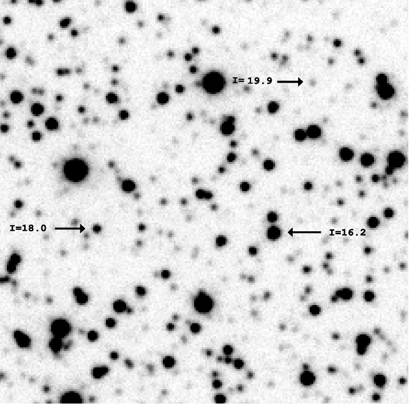
Figure 6: A sample 60${}^{\prime\prime}\times 60^{\prime\prime}$ square of a survey image. The whole MOSAIC II field is $36^{\prime}\times 36^{\prime}$, or $\sim$1400 times this area. Note that a large fraction of the stars are relatively isolated, and a significant fraction of the image area is free from stars, which still permits a good determination of the sky level. The arrows point to three stars with different magnitudes. The two at $I$ = 16.2 and 18.0 span the range of most of our stars suitable for high-precision photometry. The star with $I$ = 19.9 is too faint for $<$ 1% photometry in a single frame.

In order to choose the best field within the preselected region we take $BVRI$ test images of several fields, using the same instrument to be used for the actual search. We compute number counts and construct color-magnitude (CM) and color-color diagrams for each field, and choose the field with the best combination of the following factors: highest proportion of lower main-sequence stars, uniform and low dust extinction, and smallest number of bright stars that saturate large areas in the CCD. As an example, Figure 5 shows a color-magnitude diagram of one chip in the field of the EXPLORE I search at the CTIO 4-m telescope. An additional consideration could possibly be to choose an uncrowded stellar field so that that the photometric precision is not adversely affected by crowding. In practice, however, most Galactic plane fields are not significantly crowded for the 1–2 minute exposures and 4-m-class telescopes used in the EXPLORE project. Moreover, effective photometry algorithms have been developed to handle crowded field relative photometry (e.g., difference imaging by Alard & Lupton 1998; Woźniak 2000; Udalski et al. 2002a). Figure 6 shows an example of a small region (1/1400 of the total area) in the EXPLORE I field, which is located in the Galactic plane at $l=-27.8$, $b=-2.7$. Note that a large fraction of the stars are relatively isolated, and a significant fraction of the image area is free from stars, which permits a good determination of the sky level (crucial for faint star photometry).

An important consideration is to minimize the number of giant stars, since they are too large to be useful for planet transit detection (since $(R_{J}/R_{*})^{2}\ll 1\%$) and are a major source of contamination in shallow (mag $\lesssim$ 13), wide-field transit surveys (W. Borucki 2001, private communication; D. Latham 2001, private communication). In the case of the EXPLORE project, we minimize the proportion of contaminating giant stars in our sample by observing the Galactic plane with deep images (e.g., $15\lesssim I\lesssim 20$). A giant star would have to be nearly outside the Galaxy in order to have the faint apparent magnitude of most stars in our survey; for example, a K5 giant with an apparent magnitude of $I\sim 17$ (assuming 1 magnitude of extinction in $I$) would be at a distance of 54 kpc, where the Galactic stellar density is extremely low. Also, we select fields away from the Bulge in order to avoid bright giant stars, which would often saturate the CCD and increase crowding in the field.

Using a very red filter allows us to maximize the number of lower main-sequence stars (i.e., relatively small stars), for which transits are most easily detected for a given size planet. Specifically, an $I$-band filter increases the counts of stars of later type than the sun by a factor of 2 to 6 over that of $R$-band (for a fixed magnitude range). Observing in the $I$ band minimizes the effects of absorption by interstellar dust as compared to bluer bandpasses. Finally, the choice of the $I$ band produces light curves with the least significant limb-darkening among standard $BVRI$ filters (see Figure 2); this is extremely useful for selecting eclipses with clear flat bottoms and for deriving the best transit parameters without significant dependence on uncertain limb-darkening models (see §2).

4.3 Photometric Precision and Time Sampling

High photometric precision and high time sampling are crucial in order to identify the best set of transiting planet candidates with minimal contamination, as was described in §2. In the EXPLORE project, we achieve both high photometric precision and high time sampling by monitoring a single field throughout the observing run, with exposures taken every $\sim 3$ minutes. Care is taken so that the field position does not shift in the CCD by making small adjustments to the pointing throughout the night, and average net shifts in the field position are kept to $<1^{\prime\prime}$. This is done in order to minimize photometric errors introduced by residual differences in the CCD response across the chip that are not completely taken away by the flat-field correction, and to simplify the photometry pipeline algorithm.

Observing a single field is the strategy which achieves the highest time sampling. A more complicated strategy in which several fields are monitored at once by switching from field to field would significantly decrease time sampling of each field. Also, setting up the position and guiding of each field many times throughout the night would likely lead to a large waste of observing time. Another alternative strategy of switching fields only once or twice throughout the night would mean that each field would only be observed for 3–5 hours at a time; this would significantly reduce the transit detection efficiency $P_{vis}$, as discussed in §3.2.

We have developed a customized pipeline to perform high-precision photometry of faint stars in dense fields with a well-sampled PSF. Full details of our photometry pipeline will be described in Yee et al. (2002), and we present a brief summary of the algorithm here. A key feature of our high-precision photometry algorithm is the use of relatively small apertures (about a factor of two to three larger than the seeing disk, i.e., a diameter of 2^′′ to 3^′′) for measuring the flux. This stems from the requirement to minimize the contribution of sky noise for stars that are not significantly brighter than the sky (as faint as $I\sim 19$). The crucial consideration in obtaining high-precision relative photometry when using such small apertures is the exact placement of the center of the aperture relative to the centroid of the stars. We achieve this high-precision aperture placement by using an iterative sinc-shift algorithm to resample each star so that the central $3\times 3$ pixels sample the PSF symmetrically (Yee 1988). A photometric growth curve for each object is then derived using integer pixel apertures on the resampled image of the star. The resampling is equivalent to placing all the stars within the photometry aperture in an identical manner, allowing for relative photometry to be carried out using much smaller apertures than is customarily done. The photometric measurements of each star are then put on a relative system by comparing them to a set of reference stars determined using an iterative algorithm to find the most stable stars in a given region of the CCD. Light curves are finally produced based on the relative photometry. Examples of the high-quality light curves achieved using the first version of our pipeline are shown in Figures 7 and 8, and further discussed in §5.

4.4 Data Reduction Strategy

A key feature of the EXPLORE project is that the data reduction and analysis is done on a short timescale. In order to produce light curves within 1–2 weeks of the end of an observing run we have developed a pipeline which runs on a dedicated computer cluster. Our pipeline consists of custom-written programs to do image pre-processing, aperture photometry, relative photometry, and to generate light curves. The only steps that currently require significant human intervention are visual verification of the automatic object finding performed using the program PPP (Yee 1991) to create a star catalog, and finding the best parameters for the relative photometry. The latter step will eventually be done automatically as well. The main bottleneck that currently prevents us from reducing data in real time (which is our eventual goal) is the long time it takes to read the raw data tapes written at the telescope into the computer cluster where the data are reduced. A main motivation for the fast data reduction is that follow-up radial velocity observations of transiting planet candidates are best interpreted if done in the same season when the phase of the orbit is known. For a two week or shorter observing run, the baseline for determining the period is small so that typical errors in the period will accumulate over a year and the phase will likely be lost.

4.5 Follow-up Radial Velocity Measurements

Late M dwarfs ($M\geq 80M_{J}$), brown dwarfs ($13M_{J}<M<80M_{J}$), and gas giant planets ($M\leq 13M_{J}$) are all of similar sizes due to a competition between Coulomb force effects ($R\sim M^{1/3}$) and electron degeneracy pressure effects ($R\sim M^{-1/3}$) (Hubbard, Burrows, & Lunine 2002). Hence, transits alone are not enough to determine that a transiting companion is actually a planet even if the radius is constrained to be $\sim$ 0.1–0.15 $R_{\odot}$. Radial velocity (RV) measurements therefore are needed to determine the mass, and thus the nature, of the orbiting companion. RV measurements are also useful to rule out grazing binaries and other possible contaminants that mimic the transit signature, which can be common in the case of noisy light curves (§4.6). The transit search method with follow-up radial velocity confirmation is very powerful because every planet found has a measured radius and an absolute mass. Obtaining a mass measurement for transiting planet candidates is facilitated by the fact that the orbital period and phase are known a priori, and therefore observations can be conducted at pre-determined times such that the radial velocity differences are maximized. In the case of faint stars where planet masses lower than 1–2 $M_{J}$ cannot be detected due to limitations in the currently achievable RV precision, it is still possible to determine a mass upper limit of a few $M_{J}$ (e.g., Mallén-Ornelas et al. 2002). An actual mass measurement is generally required for confirmation of the presence of a planet. However, a mass upper limit could still be used to make a case for the presence of a planet as long as all possible contaminants to the transit signature can be ruled out with confidence (see § 4.6).

The amplitude of the RV variations of a star in the presence of a less massive companion in a circular, edge-on orbit is:

$$K=2\pi\left(\frac{G}{4\pi^{2}P}\right)\frac{m_{2}}{m_{1}^{2/3}}.$$ (8)

Here $P$ is the period and $m_{1}$ and $m_{2}$ are the primary and secondary masses, respectively. Because transiting planet orbits are seen almost completely edge-on ($i\sim 90^{\circ}$), the full RV variation is along the line of sight. A G2V star ($M=M_{\odot}$) with an 80 $M_{J}$ M dwarf or a 13 $M_{J}$ brown dwarf companion with an orbital distance $D=0.05$ AU (corresponding to $P=4.08$ days) will show RV amplitudes of 10.1 km/s and 1.6 km/s, respectively. Thus both M dwarfs and brown dwarfs are very easy to rule out with $<$ 500 m/s RV precision (even for stars more massive than G2V and for stars with planets in slightly longer period orbits). A simulated example is shown in Figure 9. Note that a radial velocity precision of 500 m/s is easily attainable with an echelle spectrograph on an 8-m-class telescope even for the relatively faint stars ($I\lesssim 18$) in the EXPLORE project.

We note that planet searches that use RV measurements to find planets reach a precision of a few m/s (e.g., Butler et al. 1996; Pepe et al. 2000). This level of precision is important when one is trying to detect possible periodic changes in the RV and measure orbital parameters, but is not necessary when trying to distinguish variations of widely different amplitudes for a system with a known period and phase. Radial velocity follow-up confirmation of transit candidates can be extremely efficient. As shown in Figure 10, only a handful of RV points at a judiciously chosen time are needed to constrain the companion’s mass, as long as the period and phase are known. Knowing the transiting companion’s orbital phase is very important when interpreting the RV measurements. A small error in the period measurement from a two-transit discovery light curve will rapidly accumulate with each orbit to give a phase error that increases linearly with time. For instance, in one year a planet with a $3\pm 0.007$ day period (i.e., a 10-minute uncertainty) will have an accumulated error of 0.85 days, or 0.3 in phase. Thus, for a $\sim$two-week observing run (with only a short baseline for period determination) it is best to do follow-up observations in the same season the discovery light curve is taken, since otherwise a second imaging run will be required a year after the discovery observations simply to recover the phase.

4.6 Minimizing Potential Contamination to the Transit Signature

It is important to select the very best candidates for the RV follow-up in order to have a high yield of planets. The three main characteristics intrinsic to transiting planet light curves are (1) they show very shallow eclipses, (2) the eclipses have a flat bottom in a bandpass where limb darkening is negligible, and (3) there is no secondary eclipse. Four different types of systems could be confused with a transiting planet: grazing eclipsing binary stars; an eclipsing binary system consisting of a large primary star with a small stellar companion; an eclipsing binary star contaminated by the light of a third blended star; and a transiting brown dwarf or late M dwarf. This section discusses the first three types of possible contaminants and some ways to differentiate them from bona-fide planet transit light curves before the RV follow-up. Contaminants of the fourth type (brown dwarfs or late M dwarfs) can only be distinguished by RV follow-up observations, but they are of great interest in their own right.

4.6.1 Ruling Out Grazing Eclipsing Binaries

At certain orbital inclinations a grazing eclipsing binary star can produce the sought-after drop in brightness of 1% when a small part of the companion crosses the primary star. If the stars are of similar surface brightness, or if one star has a much larger surface brightness than the other, then it may not be possible to discern any secondary eclipses in the data. Hence, these very shallow eclipses can be the major cause of false-positive planet candidates in some transit searches (W. Borucki 2001, private communication; D. Latham 2001, private communication). Even though the eclipse depth may be the same as a transiting planet, a grazing eclipse from a binary star system has a different shape. As illustrated in Figure 11, a triangular light curve with a rounded bottom is indicative of a grazing binary system, since the stellar companion only partially overlaps the primary star’s disk. In contrast, a transiting planet has a flat-bottomed eclipse, which indicates that the eclipsing companion is entirely superimposed on the disk of the primary star. Note that for a small range of orbital inclinations, the transiting planet is never fully superimposed on the primary star and produces an eclipse with a very similar shape and depth to that of a grazing binary (Figure 11b). However a partial transit geometry is rare for $R_{p}\ll R_{*}$, and in most cases the depth of a partial transit will be much less than 1%. Thus for practical purposes, even if partial planet transits are not included in the followup RV measurements they can be accounted for statistically.

High time sampling and high-precision photometry are required in order to determine the shape of the eclipse, and thus distinguish between the shallow round eclipses caused by grazing binary stars and eclipses with flat bottoms that may be caused by transiting planets. Distinguishing between the two types of eclipses is easiest when the light curve is taken in a bandpass which is not severely affected by limb darkening (Figure 2).

To distinguish grazing binaries from transit candidates, the EXPLORE project takes observations at a very high rate (every $\lesssim 3$ minutes), and uses an $I$-band filter so that limb darkening is not significant. Figure 7b shows an example of a grazing binary system light curve from the EXPLORE I search, as evidenced from the round bottom and highly sloped ingress and egress of the eclipses. Although grazing binaries can be trivially ruled out by follow-up RV measurements, it is essential to have flat-bottomed eclipse candidates for a high yield of actual planets among the candidates chosen for follow-up.

4.6.2 Ruling Out Eclipsing Binary Systems With a Large Primary Star

A small star eclipsing a large star can have the same eclipse depth as a Jupiter-sized planet eclipsing a sun-sized star. For example, an M4 dwarf eclipsing an F0 star will cause a 1%-deep eclipse with a flat bottom. A secondary eclipse is a definite indicator of an eclipsing binary star system regardless of the eclipse depth. However, if the surface brightness ratio of the primary to secondary star is large, the resulting secondary eclipse will not be visible in the light curve. A binary star system with a large primary is easy to rule out from the length of the eclipse alone. Figure 8a shows a clear example of a 2%-deep eclipse where the Jupiter-size planet/sun-like star hypothesis can be immediately ruled out. The eclipse has a 2.2 day period and lasts 5.5 hours, which is much longer than an eclipse caused by a planet with the same period orbiting a solar-type or smaller star. Another way to rule out eclipsing binaries with a large primary is to consider the unique solution of a light curve with two or more transits. With a light curve of sufficient photometric precision and time sampling, the stellar size and mass can be derived using the five equations in §2. Note that in the case of a giant star, the eclipse will be much longer than for a main sequence star of the same mass; solving the five equations in §2 using the wrong mass-radius relation will give a value of $R_{*}$ which is smaller than a giant star but still significantly larger than the sun. This will likely be enough to rule out the planet hypothesis, and can be confirmed using the color of the star. Alternatively, a binary star system with a large primary can also be ruled out by spectral classification of the star.

4.6.3 Ruling Out the Presence of a Contaminating Blended Star

A flat-bottomed and relatively deep eclipse from a companion star fully superimposed on its larger primary will appear shallower if light from a third blended star is present in the light curve. The contaminating blended star could be present due to a chance alignment with the eclipsing binary system or, more likely if the field is not too crowded, the contaminating star could be a component of an unresolved multiple star system.

The unique solution of a light curve with two or more transits can be used to identify an eclipse contaminated by a blended star. The length of the ingress or egress is set by a combination of $R_{c}/R_{*}$, and the projected impact parameter $\frac{D}{R_{*}}\cos i$ at which the companion crosses the center of the stellar disk (where $R_{c}$ is the radius of the eclipsing companion, $R_{*}$ is the radius of the central star, $D$ is the orbital distance, and $i$ is the orbital inclination). A 1% eclipse with an ingress and egress which are long compared to the total eclipse duration can be produced by the following two cases: (1) a planet crossing a sun-sized star with impact parameter $\frac{D}{R_{*}}\cos i\lesssim 1$ (i.e., the planet transits near the stellar limb), and (2) a small star eclipsing a sun-sized star, with additional light from a blended star contaminating the light curve. In case (1), the long ingress and egress are due to the fact that the planet transits close to the limb and is partially superimposed on the stellar disk for a relatively long time. This is illustrated in Figure 12, for the $i=86^{\circ}$ case (top line in panel a, dashed line in panels b and c). Note that only a very small range of inclinations will result in a transit with a proportionally long ingress/egress; therefore for bona fide planets, having a transit with a long ingress/egress is much less likely than one with a short ingress/egress. In case (2), the long ingress and egress are due to the fact that a larger companion will necessarily take a long time to completely cross the primary star’s limb even for a central eclipse (middle line in Figure 12a). Normally cases (1) and (2) would not be confused because the larger companion in case (2) will produce a much deeper eclipse than the small companion in case (1). However, if the light curve is contaminated with additional light from a bright blended star, the observed eclipse depth will be reduced, and thus case (2) can mimic the shallow transit in case (1). The surface brightness ratio of the primary and secondary stars in the eclipsing binary system in case (2) can easily be large enough so that the secondary eclipse is lost in the photometric noise of the blended light curve.

The case of an eclipsing binary system plus a blended star can be ruled out with by using a spectral type to complement the unique solution to the equations in §2, provided that the light curve has two eclipses with good photometric precision and time sampling. In the presence of a blended star, the unique solution gives a stellar mass and radius that are different from the mass and radius derived from the spectral type. Specifically, the unique solution will give an erroneously large primary star. This is because the inferred inclination of the orbit will result in a solution in which the planet transits close to the stellar limb and therefore seems to be going across a relatively small length of the primary star. A spectral type which is inconsistent with the primary star’s mass and radius as derived from the unique solution to the light curve is therefore a strong indication that there is a contaminating blended star.

Even without a spectral type, the planet hypothesis can be ruled out from the light curve alone in the case of an eclipsing binary system plus a blended star based on the overestimated primary radius. The large stellar radius together with the measured $\sim$ 1% transit depth will usually give a companion radius too large to be a planet. In other words, for a given eclipse length, the inferred stellar radius will be much larger than the true radius, and the system will appear to be a large star with a smaller stellar companion transiting very close to the stellar limb. The uncertainties in the parameters derived from the unique solution can be large and in some blended cases the companion can appear to have a size which is almost compatible with that of a giant planet. Therefore obtaining a spectral type prior to the RV follow-up is very worthwhile, especially when the ingress and egress of a transit are long compared to the total transit duration.

If the data are noisy, it may not be possible to rule out a contaminating star from the light curve, even if a spectral type is available. In this case, radial velocity follow-up observations can be used to rule out a planet by identifying two components in the spectrum: (1) a constant-velocity component coming from the blended star, and (2) a component from the primary star in the eclipsing binary system that will exhibit large radial velocity changes with the period and phase corresponding to the transits. If a bright guide star or laser guiding is available, it is also possible to test the blend hypothesis by obtaining a very high resolution image with an adaptive optics system to look for close companions. Typical stars in the EXPLORE search are at 1–2 kpc away, so a resolution of 0.05^′′ would be adequate to detect companions at 50–100 AU.

4.6.4 Ruling Out Other Sources of Contamination

Stellar secular variability might be thought of as a concern in the search for transits. However, a transit signal is very different from most intrinsic variability of a star. In particular, notice that a transiting planet causes a drop in brightness during only a small percentage ($<5\%$) of the total time. A large spot on the star’s surface, for example, can cause a periodic drop in stellar brightness with the stellar rotation period. However, the probability is low for the combination of the spot’s position on the star and the inclination of rotational axis to conspire to produce a drop in brightness for a time much shorter than half of the rotational period. Moreover a star with one large spot is also likely to exhibit other variability. Observations at different wavelengths should distinguish variability due to star spots from a relatively gray planet transit. See Giampapa et al. (1995) for a thorough discussion of this. Another concern might be confusion arising from brown dwarf or M dwarf eclipses; however, these are of great interest themselves and will be revealed by follow-up radial-velocity observations.

5 The EXPLORE I Transit Search

We now turn to early results from the first EXPLORE transit search. The EXPLORE I search was conducted during 11 nights on the CTIO 4-m telescope with the MOSAIC II camera, on May 30, and June 1-10, 2001. The MOSAIC II camera is made up of 8 2Kx4K thinned CCDs with 15 $\mu$m pixels, which corresponds to 0.27^′′/pixel and a $36^{\prime}\times 36^{\prime}$ field of view at the CTIO 4-m prime focus. We observed a single field near the galactic plane ($l=-27.8$, $b=-2.7$, $\alpha$=16:27:28.00, $\delta$=–52:52:40.0 J2000.0) with 100,000 stars down to $I=18.2$, and $\sim 350,000$ stars to $I=21$. At the latitude of CTIO, it was possible to observe the EXPLORE I field throughout the whole night, which resulted in as much as 10.8 hours of coverage on good nights. A total of $\sim$1800 images were obtained, although $\sim$200 of these were of very low quality due to poor weather conditions. The EXPLORE I field is located in an area of low and uniform dust extinction, and sits in the Norma patch of the OGLE microlensing search (Udalski et al. 1997). It will thus be possible to study long-term variability of objects in our sample when the OGLE data become public.

We had clear weather for approximately 6 nights, and had variable thick clouds and rain or fog during the rest of the run. For a percentage of the stars, however, the data taken during bad weather still yielded useful photometry. Our typical exposure time was 60 seconds for good conditions, and was adjusted up to compensate for cloud cover, or down if the sky was too bright due to moonlit clouds. The detector read time plus overhead was 101 seconds, so we typically obtained one photometric data point every 161 seconds, or 2.7 minutes. Out of the 100,000 stars to $I\sim 18.2$ that were initially processed, we have so far produced 37,000 light curves with 0.2–1% rms over a good night (Figure 13). Figure 14 shows a histogram of the number of stars with photometric precision better than 0.5%, 1%, and 1.5%. Our best candidates tend to have $\sim 0.5$% photometry and $15\lesssim I\lesssim 17$. Figures 7 and 8 show sample light curves.

The high photometric precision and high time sampling of our data are crucial for distinguishing between transits and grazing eclipsing binary stars (see §4.6.1), and necessary for deriving the system parameters from the light curve itself (see §2; Seager & Mallén-Ornelas 2002). Typical transit lengths for known close-in planets would be 2.5–3 hours (e.g., HD 209458 b), yielding $\sim 50$ points at minimum light to 0.2–1% precision (e.g., $7\sigma$ detections per full transit with $\delta m=0.002-0.01$). Note that a transit of an HD 209458 b-like planet ($R_{p}=1.35R_{J}$, Brown et al. 2001; see also Cody & Sasselov 2002) around a K0 star (typical for our field) will produce an easily detectable 2.6%-deep transit.

The data were reduced as outlined in §4.3 and candidates were found by visual examination within seven weeks after the observing run. The fast processing and examination of the data were done so that we could obtain radial velocity follow-up measurements on our best candidates before phase information was lost. The final analysis of the data will be done with an automatic transit-detection program, and extensive tests to determine detection thresholds and completeness. A preliminary estimate based on the window function for the poor weather conditions during our run results in $\sim$1 expected planet for the 37,000 stars examined so far. A statistical analysis and constraints on close-in giant planet frequency will follow in a later paper. We followed-up our three most promising candidates in September 2001 with 19 hours of Director’s Discretionary Time on the VLT+UVES. Details are discussed in Mallén-Ornelas et al. (2002).

We found several systems with eclipses of 1.5% to 3% depth. Three of these systems each had two flat-bottomed eclipses (EXP1J1628-52c07s24763, EXP1J1628-52c07s18161, EXP1J1628-52c01s52805). In addition, we found several eclipsing systems where the noise was too great to determine the eclipse shape. Of the three stars showing two eclipses with flat-bottoms, the first (EXP1J1628-52c07s24763) is clearly ruled out as a planet candidate because the transit is too long, implying a large primary (Figure 8a). The second system (EXP1J1628-52c07s18161) has a noisy light curve and more data are needed to confirm the transits.

The third system (EXP1J1628-52c01s52805), shown in Figure 8b, has two high-quality eclipses with clear flat bottoms. Based on follow-up radial velocity data, we now know that the eclipse is not caused by a planet (Mallén-Ornelas et al. 2002) but it is still an interesting system worth discussing. As is seen in Figure 8b, the light curve has two 3%-deep flat-bottomed eclipses due to a companion in a 2.23-day period orbit, and there is no sign of a secondary eclipse at $P$/2. The clear flat bottom eclipses indicate that the companion disk is fully superimposed on the parent star. $BVRI$ photometry and a classification spectrum indicate that this is an early K star on the main sequence ($M_{*}\sim 0.8~{}M_{\odot}$ and R$\sim 0.85$ $R_{\odot}$). A straightforward interpretation would be that the eclipsing companion is a 1.4 $R_{J}$ planet orbiting at 8 stellar radii from the parent star.

This third system’s eclipse ingress and egress are nearly the same duration as the flat part duration, which could be due to a planet with an orbital inclination such that it transits close to the stellar limb (Figure 12). However, the almost equal length ingress/egress and flat part of the light curve is a cause for concern: applying the uniqueness criteria for a two-transit light curve (§2) gives the stellar radius of an F star, while the spectral type indicates a K star. As was discussed in (§4.6.3), this is an indication of the likely presence of light from a blended companion diluting the light curve and making an otherwise deep eclipse appear shallow. Since EXP1J1628-52c01s52805 was our cleanest two-transit light curve, it was included in the follow-up radial velocity observations. The observations revealed a contaminating star with constant RV, blended with a fainter star showing RV variations with a 2.23 day period and a $\sim$60 km/s amplitude (see Mallén-Ornelas et al. 2002). Thus, for this eclipsing system, the planet hypothesis was ruled out.

6 Summary and Conclusion

The first successful detection of a planet by the transit method will mark a huge step forward in planet detection and characterization. Transit searches will allow planets to be found around a variety of stellar types and in a variety of environments. Every planet discovered by the transit method will have a measured radius and absolute mass (together with radial velocity follow-up measurements) which will provide key constraints for planetary formation and evolution models. In order to find a transiting planet, many thousands of stars must be monitored for $\gtrsim 2$ weeks with high photometric precision and high time sampling. Although many groups around the world are conducting transit searches and a few groups have produced transiting planet candidates, no planets have yet been confirmed by a mass measurement. In addition to searching for planets, transit searches are providing databases of variable star light curves with unprecedented time sampling and photometric precision. We note that these databases will also be extremely useful for finding moving objects such as asteroids, finding short-duration microlensing events such as those from free-floating planets, and generating deep images of stellar fields.

The EXPLORE project is a series of transit searches around stars in the Galactic plane using wide-field large-format CCD cameras on 4-m-class telescopes. We have presented the EXPLORE transit search strategy which involves monitoring a single low Galactic latitude field continuously with high-precision photometry for as many consecutive nights as possible. We have shown that continuous monitoring is the most efficient way to find planet transit candidates from the ground when only a few weeks of telescope time are available. One of the key aspects of our strategy is high time sampling, which allows us to use the unique solution of a light curve that has at least two flat-bottomed eclipses in order to select the very best planet candidates (e.g., by ruling out grazing binary stars). A unique aspect of our strategy among current planet transit searches is that we follow-up our transit candidates with radial velocity measurements in the same season they were discovered. This is key to interpreting the radial velocity observations because only a few radial velocity points are needed to rule out brown dwarfs and M dwarfs if the phase is known. The EXPLORE team has so far conducted a Southern search with the CTIO 4-m telescope (June 2001) with RV follow-up done on the VLT, as well as a Northern search with the CFHT 3.6-m telescope (Dec 2001) with RV follow-up done on the Keck telescope.

We have reported early results of the EXPLORE I search, which used the CTIO 4-m telescope and MOSAIC II camera for 11 nights in May/June 2001, out of which $\sim$6 had excellent weather. We have reached a photometric precision of 0.2–1% with points every 2.7 minutes for a sample of 37,000 stars in the Galactic plane at $l=-27.8$, $b=-2.7$ ($\alpha$=16:27:28.00, $\delta$=–52:52:40.0 J2000.0). For this number of stars and our limited time coverage, we expect to find $\sim$1 transiting planet. We have followed up three planet transit candidates with VLT UVES in September 2001. The results of the UVES follow-up are described in Mallén-Ornelas et al. (2002).

Figure 1: Photometric precision requirements for detecting transits of planets with different radii, as a function of stellar radius. The diagonal lines indicate the combination of planet and star radii ($y$ and $x$ axes, respectively) which will result in transit depths ($R_{p}^{2}/R_{*}^{2}$) of 0.01, 0.003, 0.001, and 0.0003 mag. If $N$ data points are available during transit, a photometric precision equal to the transit depth will result in a $N^{1/2}\sigma$ transit detection. For example, a 1% rms photometric precision will generally be sufficient to detect all planet/star radius combinations that fall above the top diagonal line.

Figure 2: Solar limb darkening dependence of a central ($i=90^{\circ}$) planet transit light curve. The planet has $R=1.4R_{J}$ (approximately that of HD 209458 b) and the star has $R=R_{\odot}$. The solid curve shows a transit light curve with limb darkening neglected. The other curves, from top to bottom (at time = 0), show central transit light curves with solar limb darkening for wavelengths (in $\mu$m): 3, 0.8, 0.55, 0.45. Although the transit depth changes at different wavelengths, the ingress and egress slope do not change significantly. The ingress and egress slope mainly depend on the time it takes the planet to cross the stellar limb.

Figure 3: Panel a: The probability $P_{vis}$ of detecting transiting planets with different orbital periods. $P_{vis}$ is calculated with the requirement that two transits must be observed. Consecutive nights of 10.8 hours each night are assumed. At each period all phases are considered; the difficulty of detecting some phases is expressed by the dips in the curves. For example, at integer periods some transits will always occur during the day and will not be detectable. The different symbols are for transit searches of different total number of nights: 21 nights (triangles), 14 nights (bars), and the actual time coverage of the EXPLORE I search (dotted line). The vertical long-dashed line indicates lower period limit of known CEGPs. Panel b: The mean $<P_{vis}>$ as a function of number of consecutive nights in an observing run. The solid line is for the requirement to detect two transits and the dashed line for one transit. Panel c: The efficiency of the $<P_{vis}>$ per night. For a two-transit requirement (solid line) the most efficient observing length (for 10.8 hours each night) is around 21 nights but the efficiency is similar for runs of 16 through 30 nights. For a single transit requirement the efficency curve (dashed line) decreases monotonically because each additional night does not add new transit detections, but the total $P_{vis}$ for one night is nonetheless tiny (see panel b).

Figure 4: A comparison of $P_{vis}$ for two different observing strategies: full night or partial night observations. The triangles show the fiducial model: $P_{vis}$ for 21 consecutive nights with 10.8 hours each night (the same curve as in Figure 3a). Panel a shows $P_{vis}$ from the fiducial model compared to $P_{vis}$ from a transit search with the same two-transit requirement and the same total observing time spread out over 76 nights with 3 hours per night. Almost no full transits are detected twice in the partial night piece-wise strategy. Panel b shows the same comparision as in panel a, but with the requirement relaxed to detect 4 half transits. Under the relaxed requirement, both search strategies will detect a larger percentage of the existing transits. However, the piece-wise search will still find far fewer transits than the 21-night search. As discussed in the text, the piece-wise transit search strategy has additional serious practical problems such as false partial transits caused by systematic errors in the photometry.

Figure 5: Color-magnitude diagram for chip 1 from the EXPLORE I field. The giant branch and main sequence are clearly visible, showing that the fraction of giant stars is small. Most stars fainter than magnitude $I=18$ are too faint for $<1$% photometry, but faint star data points in the light curves can be co-added to get better precision.

Figure 7: Two examples of the high time sampling and high photometric precision light curves from the EXPLORE I search. The rows correspond to different nights of data where the night numbers are listed at the far right of the figure. Note that the photometric precision varies from night to night and on some nights is especially poor due to clouds and bad seeing. The dome was closed on a large portion of nights 1, 5, and 11, and was closed for all of night 2. There is a one night gap in the time assignment between nights 1 and 2. Panel a: Many low-amplitude variable stars, such as this $\delta$ Scuti star, are found in our data set. Panel b: A light curve of a likely grazing eclipsing binary star from the EXPLORE I search. The round bottom and very sloped ingress and egress are indicative of a grazing binary system. The photometric precision and high time sampling of our data are good enough to rule out grazing binary stars, a common contaminant in other transit surveys (W. Borucki 2001, private communication). Notice the scale on the $y$ axis, which clearly shows that our relative photometry reaches a precision of considerably better than 1%.

Figure 8: Two eclipsing binary star systems from the EXPLORE I search. Panel a: The eclipse depth in this light curve is the same depth ($\sim 2$%) as a giant planet transiting a sun-sized star. However the long transit duration ($\sim$ 7% of the total orbital period) together with the 2.2 day orbital period indicates that the primary star has a very large radius, and therefore the companion is too large to be a planet. Panel b: A light curve showing two flat-bottomed eclipses. The eclipse depth is 3% and this star appears to have spectral type early K. The flat bottom of this light curve means that the companion is fully superimposed on the primary during the transit. As discussed in the text, the companion in this system is not a planet.

Figure 9: Model radial velocity curves (dotted lines) for companions of different mass orbiting a solar-mass star with $D=0.05$ AU (corresponding to $P=4.08$ days). Overplotted are simulated radial velocity data points for a 2.5 $M_{J}$ companion, with 100 m/s rms noise and well-spaced in phase. The adopted error bar is 100 m/s, approximately what is attainable with hour-long exposures on faint stars ($V\sim 18$) with 8m-class telescopes (Mallén-Ornelas et al. 2002). The two dotted lines in each panel show the uncertainty in orbital phase corresponding to accumulated 20-minute errors in the 4-day period over 4 months. It is evident from the top two panels that even with a radial velocity precision of $\sim$ 500 m/s, transits due to a stellar companion or brown dwarf companion can be easily ruled out. The $y$ axes are different for each panel; the dotted lines look similar in each panel because the radial velocity amplitude scales linearly with companion mass (equation (8)).

Figure 10: A simulated example showing that only a few radial velocity measurements are needed to constrain the mass of a close-in extrasolar giant planet if the phase of the eclipsing system is known. The solid lines show a model radial velocity curve for a 2.5 $M_{J}$ planet orbiting a solar-mass star at 0.05 AU (which corresponds to a 4.08 day period). Panels a–c show theoretical radial velocity points with added Gaussian noise of $\sigma=$100 m/s. Shown in each panel are 5, 10, and 30 radial velocity points, respectively. Panels d–f show the same as panels a–c but with a noise of 50 m/s.

Figure 11: A comparison of a planet transit light curve and a grazing eclipsing binary star light curve. The planet has $R=1.4R_{J}$ orbiting a star with $R_{*}=R_{\odot}$, at an orbital distance of $D=0.05$ AU, with a corresponding period of 4.08 days. The grazing binary system (thin solid line) is composed of two identical sun-like stars with twice the planet’s period. Panel a: The eclipsing binary star system light curve (thin solid line) with solar limb darkening at $I$, has a grazing angle of $85.11^{\circ}$, chosen to match a planet transit (at $i=90^{\circ}$) depth in the $I$ band (dashed line). Also shown are transit light curves neglecting limb darkening (thick solid line) and with solar limb darkening at 0.45 $\mu$m (dotted line). Panel b: The grazing eclipsing binary system light curve (thin solid line) has a grazing angle 85.024^∘ chosen to match the depth of a partial planet transit (dot-dashed line; the same partial planet transit curve is shown by the dot-dashed line in Figure 12c). Panel a illustrates that with high precision photometry and good time sampling, it should be possible to distinguish a full planet transit from a grazing binary star eclipse. Panel b shows that in the case in which a planet produces a partial transit, the light curve can be nearly identical to that produced by a grazing binary star. However, since $R_{p}\ll R_{*}$ for giant planets around sun-like stars, partial planet transits are rare.

Figure 12: Panel a: A schematic diagram of transiting planets with different orbital inclinations. First, second, third, and fourth contact are indicated. For lower inclinations the eclipses are shorter and ingress and egress are longer than for central transits. The planet and star are to scale for $R_{p}=1.4R_{J}$ and $R_{*}=R_{\odot}$. Panel b: Transit light curves for the three inclinations shown in panel a, for parameters $R_{p}=1.4R_{J}$, $R_{*}=R_{\odot}$, $D=0.05$ AU. The orbital inclinations, from top to bottom are, 85^∘, 86^∘, and 90^∘. The top curve is round-bottomed because the planet is only partially transiting the star (see panel a). At all other orbital inclinations the transit light curve is flat, indicating that the planet is fully superimposed on the parent star. Panel c: The same transit light curves shown in panel b, but with solar limb darkening at 0.8$\mu$m adopted.

Figure 13: Photometric precision from the EXPLORE I search on the CTIO 4-m MOSAIC camera. Log rms error vs. $I$ magnitude for a good chip and a not-so-good chip (with shallower electron wells), on a full good night and a full mediocre night (variable clouds and variable bad seeing) in our June 2001 run. Points below the horizontal dotted line correspond to stars with $<$1% rms photometry, which that are suitable for planet detection. On a bad night (not shown) there are no light curves with this precision. The dense clusters of points at bright magnitudes and the dense clusters of points with log rms $\sim$ 0.8 are due to saturated stars.

Figure 14: Histogram showing the number of stars with rms photometric precision better than 0.5% (solid line), 1% (dotted line), and 1.5% (dashed line).

References

- (1) Alard, C., & Lupton, R. 1998, ApJ, 503, 325
- (2)
- (3) Borucki, W. J., Caldwell, D., Koch, D. G., & Webster, L. D. 2001, PASP, 113, 439
- (4)
- (5) Borucki W. J., & Summers, A. L. 1984, Icarus, 58, 121
- (6)
- (7) Brown, T. M., Charbonneau, D., Gilliland, R. L., Noyes, R. W., & Burrows, A. 2001, ApJ, 522, 699
- (8)
- (9) Brown, T. M., & Charbonneau D. 2001, in Planetary Systems in the Universe: Observation, Formation and Evolution, IAU Symp. 202, Eds. A. Penny, P. Artymowicz, A.-M. Lagrange and S. Russel, ASP Conf. Ser. in press
- (10)
- (11) Burke, C. J., DePoy, D. L., Gaudi B. S., Marshall, J. L., Pogge, R. W. 2002, in Scientific Frontiers in Research on Extrasolar Planets, Eds. D. Demming and S. Seager, ASP Conf. Ser., in press
- (12)
- (13) Butler, R. P., Marcy, G. W., Williams, E., McCarthy, C., Dosanjh, P., & Vogt, S. S. 1996, PASP, 108, 500
- (14)
- (15) Butler, R. P., Marcy, G. W., Fischer, D. A., Vogt, S., Tinney, C. G., Jones, H. R. A., Penny, A. J., & Apps, K. 2001, in Planetary Systems in the Universe: Observation, Formation and Evolution, IAU Symp. 202, Eds. A. Penny, P. Artymowicz, A.-M. Lagrange and S. Russel, ASP Conf. Ser., in press
- (16)
- (17) Charbonneau, D., Brown, T. M., Latham, D. W., & Mayor, M. 2000, ApJ, 529, L45
- (18)
- (19) Cody, A. M. & Sasselov, D. D. 2002, ApJ, 569, 451
- (20)
- (21) Dame, T. M., Hartmann, D., & Thaddeus, P. 2001, 547, 792
- (22)
- (23) Gaudi, B. S. 2000, ApJ, 539, L59
- (24)
- (25) Giampapa, M. S., Craine, E. R., & Hott D. A. 1995, Icarus, 118, 199
- (26)
- (27) Gilliland, R. L. et al. 2000, ApJ, 545, L47
- (28)
- (29) Janes, K. 1996, JGR, 101, 14853
- (30)
- (31) Henry, G. W., Marcy, G. W., Butler, R. P., & Vogt, S. S. 2000, ApJ, 529, L41
- (32)
- (33) Holman, M., Touma, J., & Tremaine, S. 1997, Nature, 386, 254
- (34)
- (35) Howell, S. B., Everett, M. E., Esquerdo, G., Davis, D. R., Weidenschilling, S., & van Lew, T. 1999, ASP Conf. Ser. 189: Precision CCD Photometry, 170
- (36)
- (37) Hubbard, W. B., Burrows, A., & Lunine, J. I., 2002, ARAA, 40, 103
- (38)
- (39) Jenkins, J. M., Caldwell, D. A., & Borucki, W. J. 2002, ApJ, 564, 495
- (40)
- (41) Lin, D. N. C., Bodenheimer, P., & Richardson, D. C. 1996, Nature, 380, 606
- (42)
- (43) Mallén-Ornelas, G., Seager, S., Yee, H. K. C., Gladders, M., Brown, T., Minniti, D., Ellison, S. E., Mallén-Fullerton, G. 2002, in preparation
- (44)
- (45) Marcy, G. W., Cochran, W. D., & Mayor, M. 2000, in Protostars and Planets IV, Eds. V. Mannings et al. (University of Arizona Press: Tucson), 1285
- (46)
- (47) Mayor, M. & Queloz, D. 1995, Nature, 378, 355
- (48)
- (49) Mochejska, B. J., Stanek, K. Z., Sasselov, D. D., & Szentgyorgyi, A. H. 2002, AJ, 123, 3460
- (50)
- (51) Monet, D. B. A., Canzian, B., Dahn, C., Guetter, H., Harris, H., Henden, A., Levine, S., Luginbuhl, C., Monet, A. K. B., Rhodes, A., Riepe, B., Sell, S., Stone, R., Vrba, F., & Walker, R. 1998, The USNO-A2.0 Catalogue, VizieR Online Data Catalog, 1252
- (52)
- (53) Murray, N., Hansen, B., Holman, M., & Tremaine, S. 1998, Science, 279, 69
- (54)
- (55) Pepe, F., Mayor, M., Delabre, B., Kohler, D., Lacroix, D., Queloz, D., Udry, S., Benz, W., Bertaux, J.-L., Sivan, J.-P. 2000, in Optical and IR Telescope Instrumentation and Detectors, Proc., Eds., M. Iye and A. F. Moorwood, SPIE Vol. 4008, p. 582
- (56)
- (57) Quirrenbach, A., Cooke, J., Mitchell, D., & Safizadeh, N. 2001, in Planetary Systems in the Universe: Observation, Formation and Evolution, IAU Symp. 202, Eds. A. Penny, P. Artymowicz, A.-M. Lagrange and S. Russel, ASP Conf. Ser., in press
- (58)
- (59) Rasio, F. A., & Ford, E. 1996, Science, 274, 954
- (60)
- (61) Rosenblatt, F. 1971, Icarus, 14, 71
- (62)
- (63) Sackett, P. 1999, in Planets Outside the Solar System: Theory and Observations, NATO ASI, Eds. J.-M. Mariotti and D. Alloin, (Kluwer: Dordrecht), p. 189
- (64)
- (65) Schlegel, D. J., Finkbeiner, D. P., & Davis, M. 1998, ApJ, 500, 525
- (66)
- (67) Seager, S., & Mallén-Ornelas, G. 2002, submitted to ApJ, astro-ph/0206228
- (68)
- (69) Street, R. A., Horne, K., Penny, A., Tsapras, Y., Quirrenbach, A., Safizadeh, N., Cooke, J., Mitchell, D., & Cameron, A. C. 2001, in Planetary Systems in the Universe: Observation, Formation and Evolution, IAU Symp. 202, Eds. A. Penny, P. Artymowicz, A.-M. Lagrange and S. Russel, ASP Conf. Ser., in press
- (70)
- (71) Street, R. A., Horne, K., Cameron, A. C., Tsapras, Y., Bramich, D., Penny, A., Quirrenbach, A., Safizadeh, N., Mitchell, D., & Cooke, J. 2002, in Scientific Frontiers in Research on Extrasolar Planets, ASP Conf. Ser., Eds. D. Demming and S. Seager, in press
- (72)
- (73) Struve, O. 1952, The Observatory, 72, 199
- (74)
- (75) Udalski, A., Kubiak, M., & Szymanski, M. 1997, Acta Astron, 47, 319
- (76)
- (77) Udalski, A. et al. 2002a, Acta Astronomica, 52, 1
- (78)
- (79) Udalski, A., Żebruń, K., Szymański, M., Kubiak, M., Soszyński, I., Szewczyk, O., Wyrzykowski, L., & Pietrzyński, G. 2002b, Acta Astronomica, 52, 115
- (80)
- (81) Yee, H. K. C., Mallén-Ornelas, G., Seager, S., Gladders, M., & Mallén-Fullerton, G. 2002, in preparation
- (82)
- (83) Yee, H. K. C. 1991, PASP, 103, 396
- (84)
- (85) Yee, H. K. C. 1988, AJ, 95, 1331
- (86)
- (87) Woźniak, P. R. 2000, Acta Astron., 49, 223
- (88)