Sample Variance Considerations for Cluster Surveys

Abstract

We present a general statistical framework for describing the effect of sample variance in the number counts of virialized objects and examine its effect on cosmological parameter estimation. Specifically, we consider effects of sample variance on the power spectrum normalization and properties of dark energy extracted from current and future local and high-redshift samples of clusters. We show that for future surveys that probe ever lower cluster masses and temperatures, sample variance is generally comparable to or greater than shot noise and thus cannot be neglected in deriving precision cosmological constraints. For example, sample variance is usually more important than shot variance in constraints on the equation of state of the dark energy from $z<1$ clusters. Although we found that effects of sample variance on the $\sigma_{8}-\Omega_{m}$ constraints from the current flux and temperature limited X-ray surveys are not significant, they may be important for future studies utilizing the shape of the temperature function to break the $\sigma_{8}-\Omega_{m}$ degeneracy. We also present numerical tests clarifying the definition of cluster mass employed in cosmological modelling and accurate fitting formula for the conversion between different definitions of halo mass (e.g., virial vs. fixed overdensity).

1. Introduction

Clusters of galaxies are the most massive and rare virialized objects in the universe. At the high mass end, their local abundance depends exponentially on the rms of matter fluctuations and is thus a very sensitive probe of the power spectrum normalization and matter density in the universe (e.g., Evrard  1989; Frenk et al.  1990; Henry & Arnaud  1991; Lilje  1992; White et al.  1993; Eke et al.  1996; Viana & Liddle  1996; Henry  2000; Pierpaoli et al. 2001). Large cluster masses and high intracluster gas temperatures make galaxy clusters observable in X-rays out to relatively high redshifts ($z\lesssim 1$). Moreover, future Sunyaev-Zeldovich (SZ) surveys will provide homogeneous cluster samples with relatively simple selection functions out to $z\sim 3$ (e.g., Holder et al. 2000). The SZ surveys can therefore be used to study evolution of cluster abundance over an unprecedented range of redshifts. The abundance of clusters above a certain mass in a given area of the sky as a function of redshift is very sensitive to the amplitude and growth rate of perturbations as well as the comoving volume per unit redshift and solid angle. These, in turn, are sensitive to the cosmological parameters (e.g., Haiman et al. 2001). Therefore, strong constraints on the cluster normalization, matter content, and the equation of state of the Universe can, in principle, be obtained from large cluster surveys (Holder et al.  2001; Weller et al. 2001).

The potential of future cluster surveys, however, can only be realized after careful studies of all possible sources of theoretical and observational errors and biases. First and foremost, it is critical to understand the relation between observed and theoretical measures of cluster mass The mass-observable relations depend on the processes that shape the bulk properties of the intracluster medium (ICM). Extensive simulations of cluster formation have shed light onto the role of non-gravitational processes such as galactic feedback (e.g., Metzler & Evrard  1994; Navarro et al.  1995; Bialek et al.  2001; Holder & Carlstrom  2001) and radiative cooling (e.g., Muanwong et al. 2001). Both feedback and cooling appear to bring the predicted scaling relations between cluster X-ray luminosity, temperature, and mass in closer agreement with observations. However, both processes are notoriously difficult to incorporate into simulations and further numerical effort and detailed comparisons with new high-quality Chandra, XMM-Newton, and SZ observations will be needed to test whether these processes alone can explain various properties of the cluster ICM and its evolution. As was recently emphasized by Seljak (2002) and Ikebe et al. (2001), even the error budget on the local abundance is dominated by the uncertainties in conversion from theoretical to observable measures of mass.

Next in importance is the relationship between the cluster abundance in mass and cosmology. Recently, the use of very large volume cosmological simulations has led to significant improvements in our knowledge of the theoretical cluster mass function (Sheth & Tormen  1999; Jenkins et al.  2001; Evrard et al.  2002; Zheng et al.  2002). In particular, Jenkins et al. (2001) found that the mass function at cluster scales can be described by a universal analytic fit for all cosmologies and redshifts to an accuracy of $\lesssim 10-20\%$ in amplitude; this result was confirmed by Evrard et al. (2002) and Zheng et al. (2002). While there is reasonable hope that further studies will result in even more accurate parameterizations of the mass function, even the current uncertainty is not the principle remaining component of the error budget in cosmological constraints. Evrard et al. (2002) found that it is dominated by the uncertainties in conversion in mass definitions and sample (cosmic) variance. Indeed, the proliferation of different cluster mass definitions in theoretical analyses may be a source of considerable confusion and error in comparing predictions to observations (White 2001). Finally, unlike the other sources of errors discussed above, sample variance is usually neglected in theoretical and observational analyses.

In this paper, we present a statistical framework for describing the sample variance for a cosmological population of virialized objects identified at a single epoch or over a range of redshifts. We apply this formalism to evaluate the effects of the sample variance on the current and future cosmological constraints, focusing on the specific cases of constraints from the local cluster temperature function and the evolution of the cluster abundance in future SZ surveys (e.g., Holder et al. 2000). We show that uncertainties due to sample variance are comparable to or greater than the Poisson errors in many cases of future interest. Therefore, the variance should not be neglected in analyses aiming to derive precision cosmological constraints. Although we found that effects of sample variance are not significant in the interpretation of the local cluster abundance from the current flux and temperature limited X-ray surveys to determine the power spectrum normalization, it may be important for future studies based on the shape of the temperature function (Ikebe et al. 2001). We also present discussion and numerical tests clarifying the definition of mass in theoretical analyses and provide useful fitting formulas for conversions between different mass definitions.

The paper is organized as follows. In §2 we introduce the statistical formalism needed to describe sample variance and its effect on cosmological parameter estimation. We discuss cluster scaling relations and survey selection in §3. In §4 and §5, we discuss the impact of sample variance on the interpretation of the local cluster abundance and future high redshift surveys dedicated to studying the properties of the dark energy. Finally, in a series of Appendices, we give details of survey window calculations, numerical tests of the cluster mass function and bias and convenient fitting formulas for conversion between different mass definitions.

2. Statistical Formalism

2.1. Sample Covariance

Consider the general case of a population of objects selected for some property, for definiteness say their mass $M$ in some range $dM$ and assume that their number density fluctuation is related to the underlying linear mass field by a linear bias parameter

$$\delta n(M)=\bar{n}(M)b(M)\delta\,.$$ (1)

The average number density within a set of windows $W_{i}({\bf x}_{i})$ becomes

$$n_{i}=\int d^{3}x_{i}W_{i}({\bf x}_{i})[\bar{n}+\delta n_{i}]\,,$$ (2)

where we assume that the windows are normalized so that $\int d^{3}xW_{i}=1$. The sample covariance of these estimates of the true number density becomes

$${\langle n_{i}n_{j}\rangle-\bar{n}^{2}\over\bar{n}^{2}} = b^{2}\int d^{3}x_{i}\int d^{3}x_{j}W_{i}({\bf x}_{i})W_{j}({\bf x}_{j})$$

$$\quad\times\langle\delta({\bf x}_{i})\delta({\bf x}_{j})\rangle$$

$$= b^{2}\int{d^{3}k\over(2\pi)^{3}}W_{i}({\bf k})W_{j}^{*}({\bf k})P(k)\,.$$

Note that the large-scale structure of the universe makes the number density even in non-overlapping volumes covary. On top of this sample covariance one adds the usual shot noise variance which goes as $1/\bar{n}V$ fractionally.

This expression is easily generalized to the two cases of interest where one wishes to extract cosmological information from the number density as a function of mass and/or redshift. In this general case, consider the covariance to be between windows at distinct redshifts and the selection to be for distinct masses, $n_{i}(M_{i},z_{i})$ and $n_{j}(M_{j},z_{j})$. Then

$${\langle n_{i}n_{j}\rangle-\bar{n}_{i}\bar{n}_{j}\over\bar{n}_{i}\bar{n}_{j}} = b(M_{i},z_{i})b(M_{j},z_{j})D(z_{i})D(z_{j})$$ (4)

$$\quad\times\int{d^{3}k\over(2\pi)^{3}}W_{i}({\bf k})W_{j}^{*}({\bf k})P(k)\,,$$

where $D$ is the linear growth rate and we have again assumed a deterministic linear bias.

We will assume the following meaning of the terms sample covariance, sample variance and cosmic variance. For a given sample of objects, we will call the covariance between its subsamples (e.g. Eqn. [4] for subsamples of clusters in different mass or redshift bins) sample covariance. We will call the net effect of the covariance on a quantity of interest (e.g. a cosmological parameter) sample variance. Finally, for a sample that encompasses the entire observable universe, sample variance becomes cosmic variance.

2.2. Survey Windows

The calculation of the sample covariance relies on the description of the survey windows and the choice of binning in redshift and in mass. A few simple cases are of interest for estimation purposes. Since in the consideration of windows, the distinction in Eqn. (4) of redshift and mass bins does not enter, we will consider the notationally simpler case of a single redshift and mass range in Eqn. (2.1) without loss of essential generality.

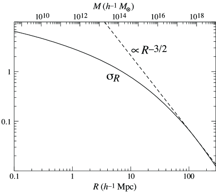
Figure 1.— Root mean square fluctuation in the linear density field $\sigma_{R}$ in the fiducial $\Lambda$CDM cosmology (§3.1) as a function of top hat radius and the corresponding enclosed mass $M=(4\pi/3)\rho_{m}R^{3}$. Because of the flatness of the linear power spectrum around $R=100h^{-1}$Mpc, the rms scales in the same way as shot noise, $V^{-1/2}\propto R^{-3/2}$ in this regime. The mass $M_{*}$ at which $\sigma_{R}=1.69$ controls the relative strength of all effects (see Figure 4).

For local surveys which cover a large fraction of the sky, it is often a reasonable approximation to take the window as a single spherically symmetric top hat volume of radius $R$. Then the variance in Eqn. (2.1) becomes

$$\sigma^{2}_{n}\equiv{\langle n^{2}\rangle-\bar{n}^{2}\over\bar{n}^{2}}=b^{2}\sigma_{R}^{2}\,,$$ (5)

where $\sigma_{R}$ is the familiar top-hat rms of linear density fluctuations field. This quantity is plotted for the fiducial $\Lambda$CDM cosmology of §3.1 in Fig. 1. Also plotted is the scaling of a white (or shot) noise power spectrum. Because the linear power spectrum is nearly flat for $R\approx 100h^{-1}$ Mpc, sample variance and shot variance scale with volume in a similar fashion for typical volumes. The sampling errors on this scale exceeds 10% for a typical bias of a few.

This basic example is readily generalized to the partially overlapping multiple spherical windows of a flux or magnitude limited selection and serves as a useful and simple order of magnitude estimate of sampling effects.

For surveys confined to a smaller section of sky but extending to cosmological distances, the windows can be divided up into slices in redshift. Consider a series of slices in redshift at comoving distance $r_{i}$ and width $\delta r_{i}$ with a field of radius $\Theta_{s}$ in radians in the small angle approximation and a flat spatial geometry:

$$W_{i}({\bf k})=2e^{ik_{\parallel}r_{i}}{\sin k_{\parallel}\delta r_{i}/2\over k_{\parallel}\delta r_{i}/2}{J_{1}(k_{\perp}r_{i}\Theta_{s})\over k_{\perp}r_{i}\Theta_{s}}\,.$$ (6)

In the limit of slices that are thick compared with the coherence,

$${\langle n_{i}n_{j}\rangle-\bar{n}^{2}\over\bar{n}^{2}}=\delta_{ij}b^{2}{1\over\delta r_{i}r_{i}^{2}}\int{d^{2}l\over(2\pi)^{2}}\left(2{J_{1}(l\Theta_{s})\over l\Theta_{s}}\right)^{2}P({l/r_{i}})\,.$$ (7)

Note that the angular window in the parenthesis goes to unity for $l\Theta_{s}\ll 1$.

Eqn. (7) is closely related to the Limber equation in Fourier space (e.g., Kaiser 1992) in that there is no covariance between distinct redshift bins and only modes perpendicular to the line-of-sight enter into the variance. We give a more general consideration of the survey window including sky curvature and a non-trivial angular mask and radial selection in the Appendix A (see Eqn. [A4]).

2.3. Statistical Forecasts

While the calculation of the covariance in the previous sections can tell us about the relative importance of sample and shot noise variance for various choices of mass and redshift binning, it does not directly translate into the relative importance on cosmological parameter estimation where the weighting of the bins reflects parameter sensitivity.

Holder et al. (2001) introduced a useful Fisher matrix approximation to a Poisson likelihood analysis which essentially propagates the errors in the bins to the covariance of more fundamental parameters. Here we generalize the technique to include sample covariance. Define the Fisher matrix in the parameter space of interest $p_{\alpha}$ as

$$F_{\alpha\beta}=\sum_{ij}{\partial\bar{n}_{i}\over\partial p_{\alpha}}({\bf C}^{-1})_{ij}{\partial\bar{n}_{j}\over\partial p_{\beta}}\,,$$ (8)

where the covariance matrix includes both sample covariance and shot variance

$$C_{ij}=\langle n_{i}n_{j}\rangle-\bar{n}_{i}\bar{n}_{j}+\delta_{ij}\bar{n}_{i}/V_{i}\,.$$ (9)

Then an estimate of the covariance matrix of the parameters follows as

$$C_{\alpha\beta}\approx({\bf F}^{-1})_{\alpha\beta}\,.$$ (10)

The Fisher approximation allows a rapid exploration of the parameter space(s) and the effect of survey specifications on statistical errors. It has been shown to be a reasonable approximation for most cosmological parameters of interest (Holder et al. 2001). Note that the parameter set can include “nuisance parameters”, e.g. an amplitude and a power law index for an observable vs. mass relation. Utilizing the Fisher matrix approximation, these parameters would be marginalized at the expense of increasing the errors

$$\sigma_{\alpha}=(C_{\alpha\alpha})^{1/2}$$ (11)

on the parameters of interest. Marginalization can be offset by prior knowledge in the form of an inverse covariance weighted sum of the information

$${\bf C}_{\rm tot}=({\bf C}^{-1}+{\bf C}^{-1}_{\rm prior})^{-1},$$ (12)

or loosely speaking by summing the Fisher matrices from individual sources. Because an infinitely sharp prior on all parameters save an $m$ element subset corresponds to considering the reduced $m\times m$ Fisher sub-matrix, we term the corresponding errors on the parameters the “unmarginalized errors”. In the case of $m=1$ parameter, the unmarginalized error is simply $1/\sqrt{F_{\alpha\alpha}}$.

Finally, for the construction of priors and the interpretation of errors it is useful to note that under a re-parameterization of the space to the set $\pi_{\mu}(p_{\alpha})$, the covariance matrix transforms as

$$C_{\mu\nu}=\sum_{\alpha\beta}{\partial\pi_{\mu}\over\partial p_{\alpha}}C_{\alpha\beta}{\partial\pi_{\nu}\over\partial p_{\beta}}\,.$$ (13)

We will use this relation to evaluate the covariance matrix involving parameters that depend on the fundamental set, e.g. $\sigma_{8}$ and the Hubble constant.

3. Cluster Surveys

We now specialize the sample variance considerations to cluster surveys in the context of spatially flat CDM models with dark energy. In §3.1, we define the cosmological framework and the parameters of interest that underly it. We provide further tests of the critical ingredients: the cluster mass function, mass definition, and bias prescription in Appendix B. In §3.2, we relate cluster observables to halo mass, providing convenient conversion formulae between different definitions of halo mass in Appendix C. These relations are used to define common selection criteria in §3.3.

3.1. Cosmological Model

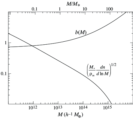
Figure 2.— Mass function and bias in the fiducial $\Lambda$CDM cosmology [see Eqns. (14) and (15)] . Although the bias increases for $M>M_{*}$ and enhances sample errors, the exponential suppression of the number densities rapidly makes shot errors dominate at $M\gg M_{*}$.

We now specialize these considerations to cluster surveys. We associate galaxy clusters with dark matter halos of the same mass. The mean differential comoving number density of dark matter halos (Jenkins et al. 2001, Eqn B3)

$${dn\over d\ln M}=0.301{\rho_{m}\over M}{d\ln\sigma^{-1}\over d\ln M}\exp[-|\ln\sigma^{-1}+0.64|^{3.82}]\,.$$ (14)

and the linear bias (Mo & White  1997; Sheth & Tormen  1999)

$$b(M)=1+{a\delta_{c}^{2}/\sigma^{2}-1\over\delta_{c}}+{2p\over\delta_{c}[1+(a\delta_{c}^{2}/\sigma^{2})^{p}]}$$ (15)

are modeled from fits to cosmological simulations with $a=0.75$ and $p=0.3$ (the values are modified to match the mass function for clusters in the Hubble volume simulations, R. Sheth, private communication). Here $\delta_{c}=1.69$ is the threshold overdensity of spherical collapse in a matter dominated universe; we will ignore the weak scaling of $\delta_{c}$ with cosmology. $\sigma^{2}(M,z)$ is the variance in the density field smoothed with a top hat that encloses a mass $M$ at the mean matter density today (or equivalently the comoving density) $\rho_{m}$. The correspondence in the adopted mass function and bias is to the mass enclosed in a region where the density is 180 times the mean matter density, as demonstrated in Appendix B. The main cosmological scaling of both the number density and bias comes through $\sigma$. It is useful then to scale the mass to $\sigma(M_{*})=\delta_{c}$. $M_{*}(z)$ is shown in Fig. 3.

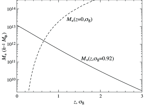
Figure 3.— $M_{*}$ controls the relative importance of sample and shot variance due to steeply declining number densities above $M_{*}$. It is a strong function of redshift and an even stronger function of normalization. The fiducial $\Lambda$CDM model assumes $\sigma_{8}=0.92$ at $z=0$ and hence $M_{*}(z=0)=1.2\times 10^{13}h^{-1}$Mpc. In conjunction with Eqn. (21), this figure can be used to determine the relative importance of sample variance for cases not explicitly explored here.

We consider the fiducial cosmology to be spatially flat and defined by 6 independent parameters: the dark energy density $\Omega_{\rm DE}=0.65$, equation of state $w=-1$, physical matter density $\Omega_{m}h^{2}=0.148$, physical baryon density $\Omega_{b}h^{2}=0.02$, tilt $n_{s}=1$, and the initial normalization of the curvature fluctuations $\delta_{\zeta}=4.79\times 10^{-5}$ at $k=0.01$ Mpc^-1 to match the COBE detection. The non-standard definition of the normalization $\delta_{\zeta}$ is given explicitly in Hu (2001) and removes the cosmological parameter dependence of the more traditional choices. For the fiducial model, it converts to $\delta_{H}=4.42\times 10^{-5}$, $\sigma_{8}=0.92$, or $M_{*}=1.2\times 10^{13}h^{-1}M_{\odot}$. We shall see that all results are a strong function of the assumed normalization but can be rescaled through $M_{*}$ (see Fig. 3 and Eqn. (21)).

3.2. Scaling Relations

The mass of a cluster is usually not measured directly, but estimated from models of its X-ray luminosity, emission weighted temperature $T_{X}$, velocity dispersion, or, in the future, its Sunyaev-Zel’dovich integrated flux.

Following Ikebe et al. (2001), we will assume an $L_{X}-T_{X}$ relation of

$$L_{X}=1.23\times 10^{37}\left({T_{X}\over 6{\rm keV}}\right)^{2.5}h^{-2}\,{\rm Wm}^{-2}\,.$$ (16)

Here $L_{X}$ is the X-ray luminosity in the energy range of $[0.1-2.4]$ keV and $T_{X}$ is emission-weighted temperature of the intracluster gas.

The connection between theoretical predictions and observations is provided by the virial mass - temperature relation $M_{v}-T_{X}$, which we parameterize as

$$\left({M_{v}\over 10^{15}h^{-1}M_{\odot}}\right) = \left[{\beta\over(1+z)(\Omega_{m}\Delta_{v})^{1/3}}{T_{X}\over 1{\rm keV}}\right]^{3/2},$$ (17)

where $\Delta_{v}$ is the virial overdensity with respect to the mean matter density (see Eqn. C6). $\beta$ parameterizes the scaling and in general may be a function of $T_{X}$ and cosmology.

Numerical simulations by various groups give $\beta\approx 0.75$ (e.g. Evrard et al.  1996; Eke et al.  1998; Bryan & Norman  1998; also Pierpaoli et al.  2001 for a tabulation of results), roughly independent of temperature and cosmology. Observations favor a lower normalization $\beta\approx 0.54(T_{X}/6{\rm keV})^{0.24}$ (Finoguenov et al.  2001) making the observed cluster sample less massive. Here we have converted from the mass at a much higher overdensity of 500 times the critical density $M_{500/\Omega_{m}}$ to $M_{v}$. The observed relation consequently indicates a lower normalization $\sigma_{8}$ in a fixed cosmology (Seljak  2002). We will employ the theoretical $M_{v}-T_{X}$ relation to be consistent with our choice of cosmology; we will discuss effects of different $M_{v}-T_{X}$ relation in §6. Since the Jenkins mass function is defined at $\Delta=180$, not at $\Delta_{v}$, the virial $M_{v}-T_{X}$ relation must be further converted to an $M_{180}-T_{X}$ relation to match with the mass function. These conversions can be done using simple but accurate fitting formulae for the general interconversion of mass definitions assuming an NFW (Navarro et al. 1997) profile given in Appendix C.

The relationship between $M_{v}$ and our $M$ can be approximately parameterized as

$$\left({M\over 10^{15}h^{-1}M_{\odot}}\right)=(1+b_{1})\left({M_{v}\over 10^{15}h^{-1}M_{\odot}}\right)^{1+b_{2}}$$ (18)

for $14<\log(M/h^{-1}M_{\odot})<16$ and halo concentrations of the fiducial model with $b_{1}=0.168x+0.373x^{4}$ and $b_{2}=0.0113x+0.0176x^{4}$ and $x\equiv 1-\Omega_{m}(z)$. Note that in the matter-dominated limit the two mass definitions coincide.

For the fiducial $\Omega_{m}=0.35$ cosmology the $M-T_{X}$ relation becomes

$$\left({M\over 10^{15}h^{-1}M_{\odot}}\right)=\left[{1.113\beta\over(1+z)(\Omega_{m}\Delta_{v})^{1/3}}{T_{X}\over 1{\rm keV}}\right]^{1.516}\,.$$ (19)

Because this $10\%$ correction in temperature will propagate into a $50\%$ correction of a flux-limited survey volume at a fixed mass, this seemingly small correction is required. Note however that the difference between simulation results for $\beta$ is at least comparable to this shift and the discrepancy between the theoretical fits to $M-T_{X}$ in simulations and observed relation (Hjorth et al.  1998; Horner et al.  1999; Nevalainen et al.  2000; Finoguenov et al.  2001; Allen et al.  2001) is more substantial still.

3.3. Survey Selection

The survey selection is a critical element in determining the importance of sample variance. Even ignoring errors in the conversion of observables to mass, which always decreases the relative importance of sample variance, the underlying cluster scaling relationships enter into the consideration of the survey selection and hence the survey window. A survey may be limited by X-ray flux, SZ flux, and/or temperature as well as volume or redshift and we will consider these as the relevant selection criteria.

For the present purpose of determining the ultimate limitation sample variance places on cluster surveys, we take the scaling relations (16) and (19) with $\beta=0.75$ to be both correct and deterministic. In reality one should include in the final error budget the intrinsic scatter, measurement, and modeling uncertainties in the observables and their relation to mass.

The $M-T_{X}$ relation allows us to convert a temperature threshold, typically $T_{X}\gtrsim 1-3$keV into a mass threshold $M>M_{\rm th}$. The combined $M-T_{X}$ and $L_{X}-T_{X}$ relations convert mass to X-ray luminosity. For sample with a flux limit $f_{\rm lim}$, the effective radius of the volume probed by the survey is

$$R={d_{L}\over 1+z}={1\over 1+z}\sqrt{L_{X}(M)\over 4\pi f_{\rm lim}}\,,$$ (20)

which implies that the survey window in mass bins will be overlapping concentric spheres or sky-wedges that increase in radius with the mass. The sample variance calculation must then properly account for the covariance between the mass bins. Note that the survey volume $V(M)\propto\beta^{-15/4}$ and hence strongly depends on the $M-T_{X}$ relation adopted. This flux limit is typically placed on top of a volume (redshift) limit that defines, for example, a local sample of clusters.

For SZ cluster surveys a flux decrement limit corresponds to $d_{A}^{-2}T_{SZ}M\approx$ const for a sufficiently large angular diameter distance $d_{A}$ such that the cluster is within the effective field of view (Holder & Carlstrom 2001). Under the assumption that the gas density weighted electron temperature $T_{SZ}\approx T_{X}$, and the $M-T_{X}$ relation above, an SZ flux limit corresponds to a mass threshold that is roughly constant with redshift and scales as $M_{\rm th}\propto\beta^{3/5}$ for different $M-T_{X}$ relations. Note that clusters of a given mass are detectable to all relevant redshifts despite the flux limit and details of the $M-T_{X}$ and $T_{X}-T_{SZ}$ relations are much less important than in a flux limited X-ray survey. Nonetheless, the $M-T_{X}$ relation has a severe effect on survey yields if the underlying power spectrum is normalized to an incorrect value by a misinterpretation of the local X-ray cluster abundance (see §6).

4. Local Abundance

We consider here the effect of sample variance compared to shot noise and cosmological parameter degeneracy on the interpretation of the local cluster abundance in the classic $\sigma_{8}-\Omega_{m}$ plane (Evrard  1989; Frenk et al.  1990; Henry & Arnaud  1991; Lilje  1992; White et al.  1993). We begin with the idealized case of a volume and temperature limited survey and then consider the more realistic X-ray flux, volume and temperature limited case.

4.1. Volume Limited Survey

Let us start with a toy model to develop intuition for the effects of sample variance. Consider a volume limited local survey with a radius $R$ that detects all clusters above a limiting mass $M_{\rm th}$ determined by a temperature limit and the $M-T_{X}$ relation.

First consider binning the clusters into a single mass bin $M>M_{\rm th}$. There is then only one window to consider and we can directly compare the sample and shot noise errors on number density determinations. Note that sample variance which is equal to shot variance leads to a $\sqrt{2}\approx 1.4$ increase in the errors.

In Fig. 4, we show the sample and shot errors for $R=100,200,300\,h^{-1}$Mpc. As noted in §2.2, in the $R=100h^{-1}$ Mpc range both errors scale as $V^{-1/2}$ and we have removed this dependence by multiplying by $(R/250h^{-1}$Mpc)^3/2. The corresponding fiducial volume is $6.5\times 10^{7}$ $h^{-3}$ Mpc³, comparable to the volume of actual local surveys. Notice that the two errors cross at $M_{\rm th}\approx 4\times 10^{14}h^{-1}\,M_{\odot}$ or $M_{\rm th}/M_{*}\approx 30$ with sample variance dominating at the lower masses. This crossing mainly reflects the exponential suppression of the number densities for $M_{\rm th}/M_{*}\gg 1$ and hence the dramatic increase in shot noise. For small changes in redshifts, normalizations, and cosmologies these qualitative statement remain true but require rescaling. Roughly,

$${M_{\rm th}\over M_{*}}\lesssim 31\left({M_{*}\over M_{*\rm fid}}\right)^{-1/2}\left(\Omega_{m}\over 0.35\right)^{1/2}\left(40\sigma_{200}\over\sigma_{8}\right)\,,$$ (21)

for sample to dominate shot variance, where recall $M_{*\rm fid}=1.2\times 10^{13}h^{-1}M_{\odot}$. For a low $\Gamma=\Omega_{m}h$ cosmology, the enhancement of sample variance from the excess large scale power (at typical scales of $R=200h^{-1}$ Mpc) from the shape of the power spectrum dominates and can substantially increase the importance of sample variance. In conjunction with Fig. 3, this scaling may be used as a rough check to determine whether sample variance is relevant to a given problem. For surveys that reach this limiting $M_{\rm th}$, sample variance will dominate over shot noise in the total number density and lead to a substantial increase in the statistical errors.

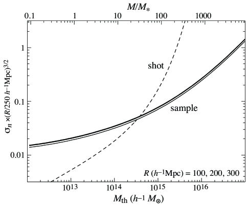
Figure 4.— Sample vs. shot errors in number counts as a function of threshold mass for a local survey. Sampling errors dominate at $M<30M_{*}\approx 4\times 10^{14}h^{-1}M_{\odot}$. Errors have been scaled by $(R/250h^{-1}$Mpc$)^{3/2}$ to reflect the local volume and the coincidence of the curves shows that both scale $V^{-1/2}$. Approximate results for alternate cosmologies or redshifts can be estimated by the scaling with $M_{*}$ (see Fig. 3 and Eqn. (21)).

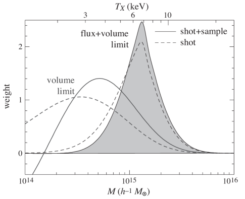
Figure 5.— Mass range sensitivity of the normalization determination for surveys with a volume limit of $z_{\rm max}$ and mass threshold of $M=10^{14}h^{-1}M_{\odot}$ with and without an additional X-ray flux limit of $f_{\rm lim}=2\times 10^{-14}$ W m². With shot noise only, the normalization constraint gets its most significant contribution for $3-4\times 10^{14}h^{-1}M_{\odot}$ ($\sim 3$ keV) for the volume limit and $10^{15}h^{-1}M_{\odot}$ ($\sim 6-7$ keV) for the additional flux limit. Correspondingly sampling errors are substantially more important for the former than the latter, also altering the optimal mass weighting (solid vs. dashed lines).

Now consider a survey that can also bin in masses, for example from individual temperature measurements. The relative contribution of sample variance will depend on what range of masses is most relevant to the question at hand. This sensitivity in turn can be a function of survey selection and cosmology. Here the Fisher matrix technique of §2.3 is useful since it automatically folds in these factors in a minimum variance weighting.

As a simple example, consider the estimation of a single parameter $p_{\alpha}$ with all others fixed by prior knowledge. The minimum variance weighting of the $i$ mass bins is given by

$$w_{i}={1\over F_{\alpha\alpha}}\sum_{j}{\partial\bar{n}_{i}\over\partial p_{\alpha}}(C^{-1})_{ij}{\partial\bar{n}_{j}\over\partial p_{\alpha}}\,.$$ (22)

For a diagonal covariance matrix as in the case of shot noise, this simply reduces to an inverse variance weighting of mass bins.

For illustrative purposes, let us take a volume limit of $z=0.09$ ($R=270h^{-1}\,$Mpc) and an all sky survey. We bin the masses from $\log(M/h^{-1}M_{\odot})=14$ to $16$ in 40 steps of $0.05$. The predicted mass function is sufficiently smooth that this binning more than suffices to recover all the information contained in its shape. Consider the parameter of interest to be the power spectrum normalization $\delta_{\zeta}$ or $\sigma_{8}$. In Fig. 5, we show the weights assuming shot noise only (dashed lines) and shot plus sample covariance (solid lines). The mass sensitivity peaks at about $3-4\times 10^{14}h^{-1}M_{\odot}$ for shot noise only implying that the inclusion of sampling errors would produce a substantial change in the error budget. Indeed the Fisher approximation yields a factor of 2 degradation in the errors on $\sigma_{8}$ or sample variance that is 3 times more important than shot variance. Other parameters, when also considered individually (unmarginalized) show similar error degradations. Note that the optimal weighting in the presence of sample covariance shifts to higher masses and can have negative contributions due to the covariance of the bins so that neglect of sample covariance in the analysis can degrade errors even further.

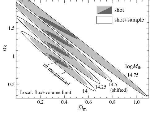
Figure 6.— $\sigma_{8}-\Omega_{m}$ constraints from a local X-ray flux and volume limited survey at $65\%$ CL ($z_{\rm max}=0.09$, $f_{\rm lim}=2\times 10^{-14}$ W m²). Unshaded ellipses denote full shot and sampling errors while shaded ellipses denote shot errors only. Outer ellipses show marginalization over other parameters (except $w$) with very weak priors, inner ellipses show the unmarginalized constraints. The four sets of $M_{\rm th}$ correspond to $T_{X}=1.25$,$1.83$,$2.67$, $3.9$ keV with the fiducial $M-T_{X}$ relation. The three higher choices of $M_{\rm th}$ have ellipses shifted in steps of $0.2$ in the $y$-direction for clarity. The effect of sample variance decreases with increasing parameter degeneracies and mass threshold.

4.2. Flux Limited Sample

More realistically, the sample of local clusters will be X-ray flux as well as volume and temperature limited so that low mass clusters are found only nearby. In this case, the mass sensitivity shifts to higher masses and sample variance becomes less important.

For illustrative purposes, let us take a flux limit of $f_{\rm lim}=2\times 10^{-14}$ W m^-2 in addition to the volume limit of $z=0.09$ and mass threshold of $M_{\rm th}=10^{14}h^{-1}M_{\odot}$ ($T_{X}=1.25$ keV), parameters typical for the current flux-limited samples of clusters with estimated X-ray temperatures (e.g., Ikebe et al.  2001). The mass weighting for the normalization parameter now peaks around $10^{15}h^{-1}M_{\odot}$ or temperatures around $T_{X}=6-7$keV with only a small difference if sample variance is included with shot variance. The degradation in normalization errors is consequently reduced to 20%. Different parameters have different sensitivities. For the chosen parameter set (see §3.1), the relative degradation in the flux limited case is largest for $\Omega_{\rm DE}$ where it reaches 40%. Thus even for a flux limited survey, sample variance can be equal to shot variance in the statistical errors.

The overall importance of sample variance can decrease due to other sources of errors in the estimation, including degeneracies in the parameters and errors in mass estimation, especially at low masses or temperatures. To illustrate these effects, consider the usual two dimensional parameter space $\sigma_{8}-\Omega_{m}$ by transforming our fundamental space as described in §2.3. In Fig. 6, we show the effect of sample variance on the 68% confidence region in this plane for several choices of the minimum mass (or temperature) in $\log(M_{\rm th}/h^{-1}M_{\odot})$ of the clusters employed, offset for the higher minimum masses for clarity. Larger ellipses represent marginalization over other parameters (with very weak priors of $\sigma_{\Omega_{b}h^{2}}=0.01$ and $\sigma_{n_{s}}=0.3$ mainly to eliminate unphysical degeneracies) and smaller ellipses represent unmarginalized constraints or prior-fixing of the other parameters. Both sets have a prior of $\sigma_{w}=0$ since the dark energy equation of state is highly degenerate with $\Omega_{m}$.

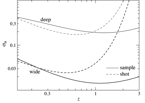
Figure 7.— Shot and sampling errors on the number density $n$ as a function of redshift for the deep ($M_{\rm th}=10^{14}h^{-1}\,M_{\odot}$, 12 deg²) and wide configurations ($M_{\rm th}=2.5\times 10^{14}h^{-1}\,M_{\odot}$, 4000 deg²). For the deep survey, sampling errors dominate shot errors out to $z\sim 0.9$, whereas for the wide survey, they cross at $z\sim 0.2-0.3$. The importance of sample variance to cosmological constraints depends on their sensitivity in redshift relative to these crossover points. Approximate results for other cases of interest can be scaled from Fig. 3 and Eqn. (21).

Not surprisingly, sample variance becomes irrelevant as the mass threshold is increased. Sample variance also decreases in importance when going between the fixed and marginalized cases due to the dominance of parameter degeneracies in the latter. For the $M_{\rm th}=10^{14}h^{-1}M_{\odot}$ threshold, the increase in the errors on $\Omega_{m}$ go from $40\%$ in the fixed case to $30\%$ in the marginalized case. The effect of marginalization mainly comes through parameters that change the shape of the linear power spectrum. Realistic current constraints on these parameters places reality approximately half-way in between the two extremes shown in Figure 6. Finally, note that the errors in the direction orthogonal to the degeneracy line increase negligibly with the addition of sample variance and threshold mass $M_{\rm th}$. Since the local cluster abundance is usually used to constrain this direction (c.f. Ikebe et al.  2001 for use of the degenerate direction), its cosmological interpretation is essentially unmodified by sample variance or uncertainties at the low mass end.

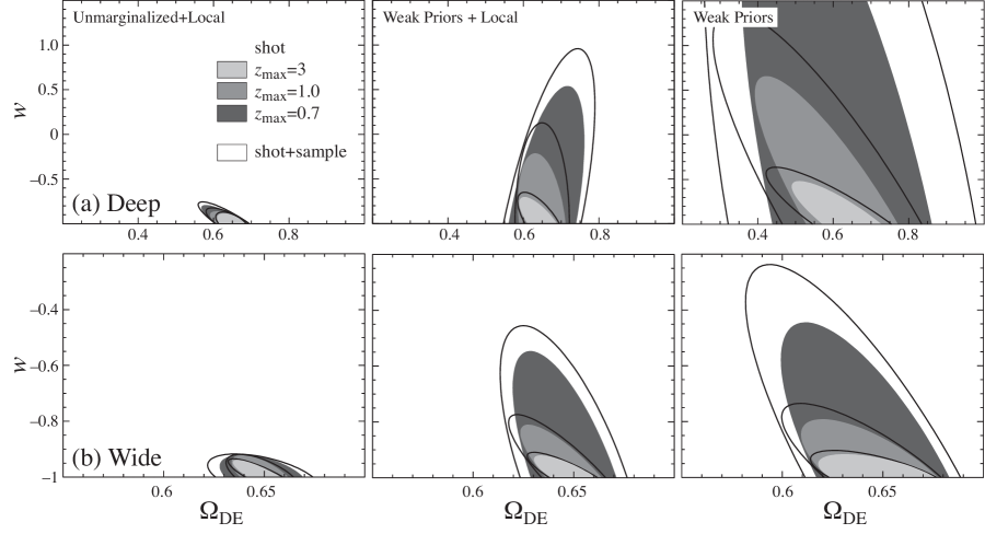
Figure 8.— Dark energy constraints (68% CL) for the (a) deep and (b) wide high redshift cluster surveys. Panels right to left reflect the addition of priors from the base set of weak conservative priors to the addition of a local cluster abundance constraint to the further addition of sharp priors on all other parameters. Three different maximum redshifts are shown with and without the inclusion of sample variance errors.

5. High-$z$ Surveys

The number abundance of high redshift clusters is widely recognized as being extraordinarily sensitive to cosmological parameters due to the exponential cut off in the mass function above $M_{*}(z)$ (Bahcall & Fan  1998; Blanchard & Bartlett  1998; Viana & Liddle  1999). Recently, its use in constraining the density and equation of state of the dark energy using planned Sunyaev-Zel’dovich (SZ) cluster surveys has been the focus of several studies (Haiman et al.  2001; Weller et al.  2001). These studies show that if the shot noise of rare high redshift clusters were the only source of uncertainty, the SZ effect can constrain the equation of state at the percent level. Here we consider the effects of additional uncertainties from sample variance and parameter degeneracies for two classes of planned surveys: a deep but narrow survey volume and a wide but shallower survey.

5.1. Fiducial Surveys

As discussed in §3.3, an SZ survey has the virtue of being able to detect clusters of a sufficiently high mass out to all redshifts that they exist. In addition, the survey selection can be described by an effective threshold mass $M_{\rm th}$ that depends only weakly on redshift (Holder et al. 2000). Following Holder et al. (2001), we take as our fiducial surveys a 12 deg² survey with a step function mass selection at $M_{\rm th}=10^{14}h^{-1}$ Mpc (“deep”) and a 4000 deg² survey to $M_{\rm th}=2.5\times 10^{14}h^{-1}$ Mpc (“wide”). We take a minimum redshift of $z=0.09$ to match the maximum redshift of the local surveys of the previous section and bin in redshift to $\Delta z=0.1$. The evolution of the number abundance is sufficiently smooth for the constant $w$ models considered that finer binning is not needed, as we find no significant degradation of constraints when varying bin size up to $\Delta z=0.1$. This is comfortably larger than the expected accuracy of individual cluster redshifts estimated using photometric redshifts of member galaxies (e.g. Fernández-Soto et al. 2002). We calculate the sample covariance under the window approximation of Eqn. (6) in both cases. Since the redshift binning corresponds to scales of $\sim 3000\Delta zh^{-1}$ Mpc, the covariance is confined to a few neighboring redshift bins but still should not be neglected. Likewise, the further Limber-like approximation of Eqn. (7) is not valid for the wide survey since line-of-sight modes contribute comparably to transverse modes for these large transverse scales. In addition, sky curvature begins to play a role for the wide survey and a more detailed analysis should employ the general window expression (Eqn. [A4]) given in Appendix A. We neglect this correction since we are mainly interested in the relative effects of sampling errors.

In Fig. 7 we show the relative contribution of shot and sample errors as a function of the redshift of the bin. Because of the low mass threshold of the deep survey, sampling errors dominate all the way out to $z\approx 0.9$. For the wide survey, the crossing occurs at $z\approx 0.2-0.3$ but sample variance remains important at $z\lesssim 0.7$. The crossing point for other cases of interest may be scaled from Eqn. (21) and Fig. 3. Whether sample variance affects cosmological constraints depends on where in redshift the parameter sensitivity is maximized.

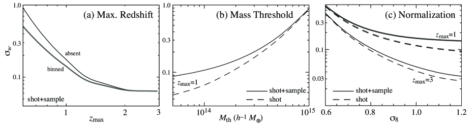
Figure 9.— Exploration of sensitivity of equation of state errors to assumptions in the wide survey and cosmology. (a) Maximum redshift with $z>z_{\rm max}$ either absent in the survey catalog or binned into a single mass bin. (b) Mass threshold for a $z_{\rm max}=1$ and (c) normalization of the linear power spectrum $\sigma_{8}$ for $z_{\rm max}=1$ and $3$. Weak priors are assumed throughout.

Even though SZ surveys have no redshift limit, the selection may still be redshift limited for two reasons: redshift followup and uncertainties in evolution. Since the SZ effect is redshift independent it also gives no intrinsic handle on the redshift of clusters so discovered. Fortunately, the relative crudeness of the binning required ($\Delta z\approx 0.1$) implies that photometric redshifts of cluster member galaxies should be more than sufficient. Still, photometric redshifts in the range $1\lesssim z\lesssim 2.5$ are difficult to obtain from optical ground-based observations. We shall see that even if redshifts cannot be determined beyond a maximum redshift $z_{\rm max}$ much of the cosmological information is recovered simply by binning all such clusters into a single high redshift bin. More worrying is any evolution in cluster properties that change $M_{\rm th}$ (or more generally the mass selection function) which cannot be accurately modeled from simulations or detailed multi-wavelength observations. In this case the clusters above a certain $z_{\rm max}$ may be unusable for cosmological constraints.

5.2. Dark Energy Constraints

Let us now specialize these considerations to the question of constraining the density $(\Omega_{\rm DE}$) and equation of state ($w$) of the dark energy. Constraints in this plane and the relative importance of sample variance are far more sensitive to prior assumptions on other cosmological parameters than the normalization from the local abundance. We choose three levels of prior knowledge: (1) Weak priors that reflect a conservative view of current cosmological constraints $\sigma_{h}=0.065$, $\sigma_{\Omega_{b}h^{2}}=0.01$, $\sigma_{n_{s}}=0.3$, $\sigma_{\ln\zeta}=2$, (2) Weak priors plus a local cluster abundance constraint from §4 for the flux and volume limited case, and (3) Unmarginalized errors with the addition of the local cluster abundance constraint.

In Fig. 8, we show the resulting constraints for the deep and wide surveys and maximum redshifts of $z_{\rm max}=0.7$, $1.0$ and $3$. For the deep surveys and weak priors, degradations in the errors on ($\Omega_{\rm DE}$, $w$) change slightly from (1.3,1.3) to (1.4,1.4) to (1.4,1.3) as $z_{\rm max}$ increases. The degradation decreases [(1.3,1.3) to (1.1,1.4) to (1.1,1.2)] once the local abundance is added to a high $z_{\rm max}$ make the constraints less dependent on the sample variance limited low redshift end. Fixing other parameters reduces the effect still further. Note that the effect of priors on the absolute errors is much larger than on the relative effect of sample variance. For the wide survey the degradation decreases from (1.3,1.4) to (1.1,1.2) as $z_{\rm max}$ increases with weak priors and changes to (1.2,1.2) to (1.2,1.1) with the addition of the local abundance constraint. These smaller degradation factors reflects the overall decrease in the importance of sample variance with increasing mass threshold. In summary, sample variance causes a 10-40% degradation in dark energy constraints depending on the detailed assumption made. Since 40% reflects equal shot and sample variance contributions, sample variance cannot be ignored in the statistical error budget of future surveys. Moreover it can affect the optimal survey strategy given fixed observing constraints, e.g. making it more important to study rare high redshift clusters.

Let us further explore these issues in the context of the wide survey, weak priors and the measurement of the equation of state parameter $w$. Both the absolute constraints on $w$ and the relative importance of sample variance are very sensitive to three quantities: the maximum redshift $z_{\rm max}$, the mass threshold $M_{\rm th}$, and the fiducial value of the normalization $\sigma_{8}$ (see Fig. 9). Note the sharp increase in the errors for $z_{\rm max}<1$. If the maximum redshift simply reflects a lack of followup redshift information beyond this redshift, a fair fraction of the lost information can be regained just by binning all such clusters into a single high redshift bin. A low mass threshold at high redshift is also critical for obtaining strong constraints on $w$ and also increases the relative importance of sample variance. Finally the assumed normalization of the cosmological model has a strong effect on the errors on $w$ due to the lack of high redshift clusters as the normalization decreases. A lowering of the normalization by a factor of $0.8$ changes the errors on $w$ by nearly a factor of 3. Lowering the normalization also reduces the importance of sample variance as clusters become rarer, especially at high redshift.

6. Discussion and Conclusions

The analyses presented in the preceding sections showed that for future surveys that probe ever lower cluster masses and temperatures, sample variance is generally comparable to or greater then the shot noise and thus cannot be neglected in deriving precision cosmological constraints. For example, sample variance typically doubles the statistical uncertainty in constraints on the dark energy equation of state in a SZ survey limited to $z_{\rm max}\lesssim 1$. Its relative importance is very weakly dependent on survey volume and is mainly a decreasing function of mass threshold of the survey, $M_{\rm th}$, compared with the mass of a typical halo, $M_{*}$, because of the rarity of high mass clusters. We emphasize though that it is simply that the shot noise variance for future surveys is impressively small, and the cosmological prospects correspondingly bright, that the small absolute effect of sample variance plays any role at all!

Although we found that effects of sample variance on the $\sigma_{8}-\Omega_{m}$ constraints from the current flux and temperature limited X-ray surveys of local clusters are not significant, they may be important for future studies utilizing shape of the temperature function to break the $\sigma_{8}-\Omega_{m}$ degeneracy, where sample variance typically increases the statistical variance by a factor of two.

We have studied the effects of sample variance under the assumption that the fiducial $\Lambda$CDM cosmology is essentially correct and, most importantly, its joint normalization to the COBE results and cluster abundance assuming the usual simulation-based conversion of X-ray temperature to mass. Recent improvements in the measurement of the observed mass-temperature relation has called the latter assumption into question (Finoguenov et al.  2001, Ikebe et al.  2001). Because of the extraordinary sensitivity of cluster survey yields to the normalization of the power spectrum, these developments can significantly alter the prospects of cluster surveys including the relative importance of sampling variance. Employing the observed relation from Finoguenov et al. (2001) and fixing the number of clusters at $T_{X}>6$ keV in our idealized flux and volume limited surveys, we find that the normalization of the fiducial cosmology would be lowered to $\sigma_{8}=0.75$ from $0.92$, in agreement with conclusions of Seljak (2002).

This change has opposite consequences for the importance of sample variance for the local and high-redshift surveys. For the local surveys, since the number density in temperature is fixed, the decrease in the mass threshold, $M_{\rm th}$ increases the importance of sample variance (see Eqn. [21]). For example, degradation in the unmarginalized errors on $\Omega_{\rm DE}$ increases from $1.4$ to $1.6$. Sample variance effects would be even larger if the model is also tilted to match the COBE normalization. For the high-redshift surveys, the weak scaling of mass threshold with the mass-temperature relation (see § 3.3) and strong scaling of constraints with normalization (see Fig. 9) make sample variance less important compared to our analyses. More importantly, the change in the normalization relation would substantially degrade the ability of SZ surveys to measure dark energy properties due to the increase in the rarity of high redshift clusters. These relative changes remain true if the mass-temperature change indicates a higher dark energy density $\Omega_{\rm DE}\approx 0.75$, $\Omega_{m}h^{2}=0.13$, with a $\sigma_{8}=0.85$ that then matches the COBE normalization as well as the $T_{X}>6$ keV cluster abundance.

This current ambiguity in predictions reflects the general point that until the mass-observable relationships for clusters are well understood with new observations and better simulations, the predicted cosmological yield of future cluster surveys and the statistical error budgets considered here should be taken as highly uncertain. These relationships therefore should be the primary focus of the future modeling efforts and can be attacked in several ways. First, the use of higher resolution and more sophisticated cluster simulations together with new high-quality Chandra and XMM-Newton observations should fuel progress in our understanding of cluster scaling relations in the near future. The search for causes of discrepancy between the observed and predicted $M-T_{X}$ relations that currently compromises interpretation of the local cluster abundances, is already the subject of substantial observational and modeling effort. At the same time, independent constraints on mass-observable relations can, in principle, be obtained from weak lensing analyses of large X-ray selected cluster samples. In addition, power spectrum normalization at cluster scales can be obtained independently from studies of cosmic shear (e.g. Van Waerbeke et al. 2002). Independent measurement of $\sigma_{8}$ would allow use of local cluster temperature function to constrain present-day $M-T_{X}$ relation. Although at higher redshifts prospects are less promising for the immediate future, deep X-ray and SZ follow-up observations to the SZ surveys should provide a wealth of data on such cluster populations. These data will be critical for comparisons with numerical simulations, tests of the scaling relations evolution, and, ultimately, precision cosmological constraints from cluster surveys.

Acknowledgments: We thank J. Carlstrom, Z. Haiman, G. Holder, J.J. Mohr, C. Pryke, A. Evrard, and M. White for stimulating conversations. WH was supported by NASA NAG5-10840 and the DOE OJI program.

Appendix A Window Function

We outline here the calculation in the case of a general survey window. Consider a general radial selection $R_{i}(r)$ and angular mask $\Theta(\theta,\phi)$ such that the set of windows satisfies the separability condition $W_{i}({\bf x})\equiv R_{i}(r)\Theta(\theta,\phi)$. The Fourier transform of the window then becomes

$$W_{i}({\bf k})=4\pi\sum_{lm}(-i)^{l}\tilde{R}_{i\,l}(k)\tilde{\Theta}_{lm}Y_{l}^{m}(\theta_{k},\phi_{k})$$ (A1)

and ($\theta_{k}$,$\phi_{k}$) define the direction of ${\bf k}$ with respect to a fiducial direction, e.g. the center of the window. Here the spherical harmonic transform of the angular mask is

$$\tilde{\Theta}_{lm}=\int d\Omega Y_{l}^{m*}(\theta,\phi)\Theta(\theta,\phi)\,,$$ (A2)

and the spherical Bessel transform of the radial window is

$$\tilde{R}_{i\,l}(k)=\int r^{2}drj_{l}(kr)R_{i}(r)\,.$$ (A3)

The covariance becomes

$${\langle n_{i}n_{j}\rangle-\bar{n}^{2}\over\bar{n}^{2}}=b^{2}\sum_{lm}4\pi\int{dk\over k}\tilde{R}_{i\,l}(k)\tilde{R}_{j\,l}(k)|\tilde{\Theta}_{lm}|^{2}{k^{3}P(k)\over 2\pi^{2}}\,.$$ (A4)

In the Limber approximation of a slowly varying $P(k)$, one can use the identity

$$\int k^{2}dkj_{l}(kr)j_{l}(kr^{\prime})={\pi\over 2r^{2}}\delta(r-r^{\prime})\,,$$ (A5)

to show that the covariance is negligible

$${\langle n_{i}n_{j}\rangle-\bar{n}^{2}\over\bar{n}^{2}}=\delta_{ij}b^{2}\int r^{2}drR_{i}^{2}(r)\sum_{lm}|\tilde{\Theta}_{lm}|^{2}P(l/r)\,.$$ (A6)

Further specializing to azimuthally symmetric windows with a normalized radial tophat profile,

$${\langle n_{i}n_{j}\rangle-\bar{n}^{2}\over\bar{n}^{2}}=\delta_{ij}b^{2}{1\over r_{i}^{2}\delta r_{i}}\sum_{l}{2l+1\over 4\pi}\tilde{\Theta}_{l}^{2}P(l/r)\,,$$ (A7)

where the angular window is

$$\tilde{\Theta}_{l}=2\pi\int_{-1}^{1}d\cos\theta P_{l}(\cos\theta)\Theta(\theta)\,.$$ (A8)

In the limit that $l\gg 1$ this expression agrees with the pillbox window Eqn. (7). Note that the angular windows in both expressions are normalized to unity for $l\Theta_{s}\ll 1$, where $\Theta_{s}$ is the typical angular dimension of the window.

Appendix B Numerical tests

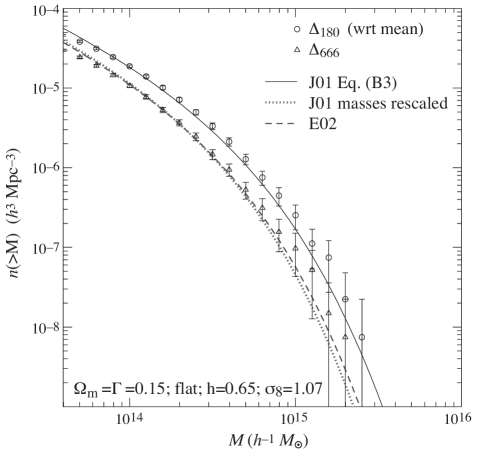
Figure 10.— Cluster mass functions derived from the simulation of a flat low-$\Omega_{m}$ CDM cosmology ($\Omega_{m}=1-\Omega_{\rm DE}=\Gamma=0.15$; $h=0.65$; $n_{s}=1$; $\sigma_{8}=1.07$) using masses defined by $\Delta_{180}$ and $\Delta=666.6$. The error bars show $2\sigma$ Poisson errors. The solid line shows the fit obtained by Jenkins et al. (2001, their Eqn. B3) while the dotted line shows this fit with $M_{180}$ converted to $M_{666}$, as described in the Appendix C. Agreement indicates that the Jenkins et al. fit should be interpreted as $M_{180}$, defined with respect to the mean density and that the mass function is universal for this definition of mass. The converted mass function fit matches both our simulated mass function for $\Delta=666$ and the fit of Evrard et al.  (2002, their Tab. 1) to the mass function from the Hubble volume $\Lambda$CDM simulation with this definition of mass. The agreement shows that conversion assuming an NFW profile adequately accounts for the substantial differences between $M_{180}$ and $M_{666}$.

During the past several years there has been significant advances in our understanding of halo mass function and bias from simulations (e.g., Mo & White 1996; Sheth & Tormen 1999; Jenkins et al. 2001). Nevertheless, there remains a certain confusion about the meaning of mass in the mass function expressions, sufficiently significant to make analyses of cluster abundances ambiguous (White 2001). Furthermore, bias models were extensively tested against numerical simulations, but only for relatively small halo masses, $M\lesssim 10-20M_{\ast}$ (Mo et al. 1997; Jing 1999; Sheth & Tormen 1999), which for our fiducial model corresponds to masses $\lesssim 2.6\times 10^{14}h^{-1}\ {\rm M_{\odot}}$. In cluster studies, especially those at high redshift, halo masses $M>20M_{*}$ must be interpreted and hence we test the bias model over the whole range.

In this Appendix we use results of a large $N$-body simulation to test the mass function and halo bias expressions used in our analyses. The simulation followed evolution of $256^{3}\approx 1.6\times 10^{7}$ particles in the flat CDM model with vacuum energy: $\Omega_{m}=1-\Omega_{\rm DE}=0.15$; $h=0.65$; $n_{s}=1$; $\sigma_{8}=1.068$; $\Gamma=0.15$; $L_{\rm box}=512h^{-1}\ M_{\odot}$. Here $\Gamma$ is the shape parameter in the adopted approximation of the initial power spectrum (Bardeen et al. 1986). The simulation was run with the Adaptive Refinement Tree code (Kravtsov et al. 1997) using $256^{3}$ zeroth level grid and five levels of refinement. The power spectrum normalization, $\sigma_{8}$, was chosen to satisfy constraints from the local cluster abundance (e.g., Pierpaoli et al. 2001).

The adopted cosmological model is sufficiently different from the models studied by Jenkins et al. (2001) to make our analysis a useful test of the universality of the mass function fit advocated by these authors. In addition, differences between various common definitions of halo mass increase for lower values of $\Omega_{m}$. For example, consider the halo mass defined within the radius corresponding to the fixed overdensity with respect to mean density of the Universe, $M_{180}=(4\pi/3)R_{180}^{3}\Delta_{180}\rho_{m}$ where $\Delta_{180}=180$ independent of cosmology. It is is equivalent to the definition of mass with respect to the cosmology-specific virial overdensity given by the spherical collapse model, $M_{v}=(4\pi/3)R_{v}\Delta_{v}\rho_{m}$ only for $\Omega_{m}=1$ because then $\Delta_{180}=\Delta_{v}$ (see Eqn. C6). For low $\Omega_{m}$, $\Delta_{180}$ and $\Delta_{v}$ are significantly different. For $\Omega_{m}=0.15$, for example, $\Delta_{v}\approx 532$. This translates into $\approx 30\%$ difference in mass for $M_{\rm vir}=5\times 10^{14}h^{-1}\ {\rm M_{\odot}}$ (see Appendix C). This cosmology provides a sharp test of the Jenkins et al. (2001) assertion that the mass function of halos defined at $\Delta_{180}$ is independent of cosmology.

Figure 10 shows the halo mass functions derived from the simulation using masses defined for $\Delta_{180}$ and $\Delta=666.6$. The latter definition was used by Evrard et al. (2002) to get fits to the mass functions in the Hubble volume simulations (it corresponds to their definition of mass at the overdensity of 200 with respect to the critical density for $\Omega_{m}=0.3$: $200/0.3\approx 666.6$). The solid line shows the fit obtained by Jenkins et al. (2001, their Eqn. B3 for this definition of mass), while the dotted line shows this fit with $M_{180}$ converted to $M_{666}$, as described in the Appendix C. The figure clearly shows that halo mass in the universal Jenkins et al. fit should be interpreted as $M_{180}$, where the overdensity of 180 is defined with respect to the mean density. The converted mass function fit matches both our simulated mass function for this overdensity and the fit of Evrard et al. (their Table 1). While it is clear that the differences in mass definition lead to substantial differences in the amplitude and shape of the mass function, Fig. 10 shows that these differences can be taken into account by the appropriate mass conversion.

Figure 11 compares the average bias for halos of mass $>M$ in simulations to the predictions of analytic models of Mo & White (1996) and Sheth & Tormen (1999). The bias in these models in linear regime is given by Eqn (15) with $(p,a)=(0,1)$ and $(0.3,0.75)$, respectively. The analytic predictions were computed as a mass function weighted average of the linear bias predictions, with the mass function fit of Jenkins et al. (2001). In the simulation, the bias was estimated as the average ratio of halo-mass and mass-mass correlation functions at linear scales: $\langle b(>M)\rangle=\langle\xi_{hm}/\xi_{mm}\rangle_{\rm lin}$. Namely, we estimated $\xi_{mm}(r)$ and $\xi_{hm}(r,>M)$ for halos with masses greater than $M$ (varying $M$ over the entire probed range of masses; $M$ here is defined for $\Delta=180$). The bias was estimated by averaging $\xi_{hm}/\xi_{mm}$ over $20-30h^{-1}\ {\rm Mpc}$ where bias is scale-independent. This gives us an estimate of the mass function weighted bias as a function of halo mass. The figure shows that both models reproduce the mass dependence of halo bias for cluster masses. The value of the bias, however, is much better matched by the model of Sheth & Tormen (1999) in all but the highest mass bins. The number of clusters in these bins is rather small (the last mass bin contains only 3 clusters) and the deviations are not significant. The figure shows that Eqn. (15) provides an accurate description of bias for the cluster mass halos.

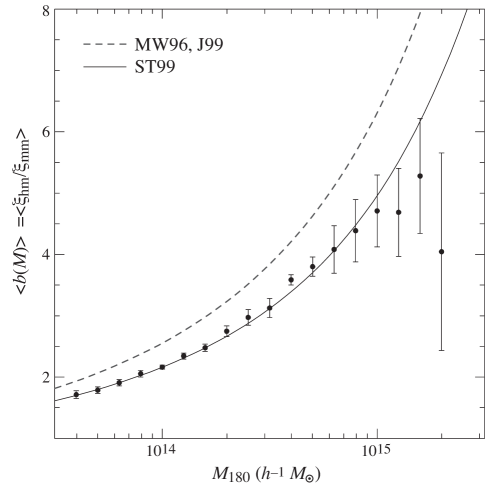
Figure 11.— The average bias for halos of mass $>M_{180}$ predicted by the analytic models of Mo & White (1996, dashed line) and Sheth & Tormen (1999, solid line), as averaged over the Jenkins et al. (2001) mass function, and in the simulation (see Fig. 10), estimated from the average ratio of halo-mass and mass-mass correlation functions at linear scales: $\langle b(>M)\rangle=\langle\xi_{hm}/\xi_{mm}\rangle_{\rm lin}$, as described in the text. The $2\sigma$ error bars are the Poisson errors in $\xi_{mm}$ and $\xi_{hm}$ propagated to $b$. Note the points are not independent because they are derived from the same simulation and use overlapping cluster catalogs.

Appendix C Mass Conversion

Various definitions of the mass of a halo can be converted assuming a halo density profile. Here we provide a fit to the general scaling function that converts definitions under the assumption of a NFW profile (Navarro et al. 1997).

The NFW halo profile has the functional form

$$\rho(r)={\rho_{s}\over(r/r_{s})(1+r/r_{s})^{2}}\,,$$ (C1)

for which the mass enclosed at a radius $r_{h}$ is

$$M_{h}=4\pi\rho_{s}r_{h}^{3}f(r_{s}/r_{h})\,,$$ (C2)

where

$$f(x)=x^{3}[\ln(1+x^{-1})-(1+x)^{-1}]\,.$$ (C3)

The limiting behavior of this function is

$$\lim_{x\rightarrow 0}f(x) = -[1+\ln(x)]x^{3}\,,$$

$$\lim_{x\rightarrow\infty}f(x) = {1\over 2}x-{2\over 3}\,,$$ (C4)

which says that if $r_{h}\gg r_{s}$ then up to a logarithmic correction, the mass converges to that enclosed near the scale radius $r_{s}$ and if $r_{h}\ll r_{s}$ the mass increases as $r_{h}^{2}$

A common baseline definition of mass for comparison is the virial mass

$$M_{v} \equiv {4\pi r_{v}^{3}\over 3}\Delta_{v}\rho_{m}\,,$$ (C5)

$$= 4\pi\rho_{s}r_{v}^{3}f(1/c)\,,$$

where the concentration parameter $c\equiv r_{v}/r_{s}$ and $\Delta_{v}$ is virial overdensity with respect to the mean matter density (Bryan & Norman 1998)

$$\Delta_{v}\approx{18\pi^{2}+82x-39x^{2}\over 1+x}\,,$$ (C6)

where $x\equiv\Omega_{m}(z)-1$. We will give the conversion from an arbitrary definition of the halo mass to the virial mass although the procedure is completely general.

Defining the halo mass as

$$M_{h}\equiv{4\pi r_{h}^{3}\over 3}\Delta_{h}\rho_{m}\,,$$ (C7)

where $\Delta_{h}$ can depend on cosmology but not on $M_{h}$, we relate the two radii as

$$f(r_{s}/r_{h})={\Delta_{h}\over\Delta_{v}}f(1/c)\,,$$ (C8)

so that

$${r_{s}\over r_{h}} = x\left(f_{h}={\Delta_{h}\over\Delta_{v}}f(1/c)\right)\,.$$ (C9)

Converting between definitions of mass simply involves inverting $f(x)$ of Eqn. (C3) to find $x(f)$ and hence an explicit formula for the relationship between two different definitions of $r_{h}$ or $M_{h}$

$${M_{h}\over M_{v}} = {\Delta_{h}\over\Delta_{v}}\left(r_{h}\over cr_{s}\right)^{3}\,.$$ (C10)

The function $f(x)$ is monotonic its single argument $x$ and it is simple to form a numerical lookup table for its inverse. Nonetheless we here provide an accurate fitting formula for the inversion

$$x(f) = \left[a_{1}f^{2p}+\left({3\over 4}\right)^{2}\right]^{-1/2}+2f\,,$$ (C11)

where $p=a_{2}+a_{3}\ln f+a_{4}(\ln f)^{2}$ and the 4 fitting parameters are $(a_{1},\ldots,a_{4})=(0.5116,-0.4283,-3.13\times 10^{-3},-3.52\times 10^{-5})$. This fit converts masses to better than $1\%$ accuracy across concentrations $0<c<400$ ($2.5<M_{v}/h^{-1}M_{\odot}<\infty$ in the fiducial model; for galaxy and cluster scales $c<20$, the conversion has typical errors of $\sim 0.3$%). Note that the inversion is exact for $c\rightarrow 0$ ($f\rightarrow\infty$) by construction.

An alternate form that is exact in the limit $c\rightarrow\infty$ can be obtained via Taylor expansion as

$${M_{h}\over M_{v}}=1+g(c,(\Delta_{h}/\Delta_{v})^{1/3})\,,$$ (C12)

where

$$g(x,y) = -3(x+y)[x-xy+(1+x)(x+y)\ln(1+x)$$ (C13)

$$-(1+x)(x+y)\ln(1+x/y)]$$

$$\times[3(1+x)(x+y)^{2}\ln(1+x)$$

$$-x(x+4x^{2}+6xy+3y^{2})]^{-1}\,,$$

and for order unity $y$ exceeds the accuracy of Eqn. (C11) for $c>10$.

These formulas allow for a convenient mapping of $M_{v}\rightarrow M_{h}$ once $c(M_{v})$ is specified. Following Bullock et al. (2001), we take

$$c(M_{v})=9(1+z)^{-1}(M_{v}/M_{*})^{-0.13}$$ (C14)

where $M_{*}$ is evaluated at the present epoch $z=0$. These formula also provide an accurate inverse relation $M_{h}\rightarrow M_{v}$. Note that in the limit $c(M_{v})\rightarrow\infty$, the mass correction is small and in the limit $c(M_{v})\rightarrow 0$, it is independent of $c$. Therefore, to obtain an accurate inverse mapping one can utilize $c(M_{h})$ in the inversion equation (C10) to obtain $M_{v}(M_{h})$ to $\sim 1\%$ across all concentrations. For better accuracy one can iterate the procedure as $c(M_{v}(M_{h}))$.

References

- (1)
- (2) Allen, S.W. Schmidt, R.W. Fabian, A.C. 2001, MNRAS, 328, L37.
- (3) Bahcall, N.A. Fan, X. 1998, ApJ, 504, 1.
- (4) Bardeen, J.M. Bond, J.R. Kaiser, N. Szalay, A.S. 1986, ApJ, 304, 15.
- (5) Bialek, J.J. Evrard, A.E. Mohr, J.J. 2001, ApJ, 555, 597.
- (6) Blanchard, A. Bartlett, J.G. 1998, A&A, 332, L49.
- (7) Bryan, G.L. Norman, M.L. 1998, ApJ, 495, 80.
- (8) Bullock, J.S. et al. 2001, MNRAS, 321, 559.
- (9) Eke, V. Cole, S. Frenk, C.S. 1996, MNRAS, 282, 263.
- (10) Eke, V. Cole, S. Frenk, C.S. Henry, P.J. 1998, MNRAS, 282, 263.
- (11) Eke, V. Navarro, J.F. Frenk, C.S. 1998, ApJ, 503, 569.
- (12) Evrard, A.E. 1989, ApJ, 341, L71.
- (13) Evrard, A.E. Metzler, C.A. Navarro, J.F. 1996, ApJ, 469, 494.
- (14) Evrard, A.E. et al. 2002, ApJ, submitted, astro-ph/0110246.
- (15) Fernández-Soto, A. Lanzetta, K.M. Chen, H.-W. Levine, B. Yahata, N. 2002, MNRAS, 330, 889.
- (16) Finoguenov, A. Reiprich, T.H. Bohringer, H. 2001, A&A, 368, 749.
- (17) Frenk, C.S. White, S.D.M. Efstathiou, G. Davis, M. 1990, ApJ, 351, 10.
- (18) Haiman, Z. Mohr, J.J. Holder, G.P. 2001, ApJ, 553, 545.
- (19) Henry, J.P. Arnaud, M. 1991, ApJ, 372, 410.
- (20) Henry, J.P. 2000, ApJ, 534, 565.
- (21) Hjorth, J. Oukbir, J. van Kampen, E. 1998, MNRAS, 298, L1.
- (22) Holder, G. Carlstrom, J.E. 2001, ApJ, 558, 515.
- (23) Holder, G. Haiman, Z. Mohr, J.J. 2001, ApJ Lett., 560, 111.
- (24) Holder, G.P. Mohr, J.J. Carlstrom, J.E. Evrard, A.E. Leitch, E.M. 2000, ApJ, 544, 629.
- (25) Holder, G.P. Carlstrom, J.E. 2001, ApJ, 558, 515.
- (26) Horner, D.J. Mushotzky, R.F. Scharf, C. 1999, ApJ, 520, 78.
- (27) Hu, W. 2002, Phys. Rev. D, 65, 023003.
- (28) Ikebe, Y. Reiprich, T.H. Boehringer, H. Tanaka, Y. Kitayama, T. 2001, A&A, in press, astro-ph/0112315.
- (29) Jenkins, A. et al. 2001, MNRAS, 321, 372.
- (30) Jing, Y.P.. 1999, ApJ, 503, L9.
- (31) Kaiser, N. 1992, ApJ, 388, 272.
- (32) Kravtsov, A.V. Klypin, A.A. Khokhlov, A.M. 1997, ApJ Suppl., 111, 73.
- (33) Lilje, P.B. 1992, ApJ, 386, L33.
- (34) Metzler, C.A. Evrard, A.E. 1994, ApJ, 437, 564.
- (35) Mo, H.J. White, S.D.M. 1996, MNRAS, 282, 347.
- (36) Mo, H.J. Jing, Y.P. White, S.D.M. 1997, MNRAS, 284, 189.
- (37) Muanwong, O. Thomas, P.A. Kay, S.T. Pearce, F.R. Couchman, H.M.P. 2001, ApJ, 552, 27.
- (38) Navarro, J.F. Carlos, C.S. White, S.D.M. 1995, MNRAS, 275, 720.
- (39) Navarro, J.F. Carlos, C.S. White, S.D.M. 1997, ApJ, 490, 493.
- (40) Nevalainen, J.. Markevitch, M.. Forman, W. 2000, ApJ, 532, 694.
- (41) Pierpaoli, E. Scott, D. White, M. 2001, MNRAS, 325, 77.
- (42) Seljak, U. 2002, MNRAS, submitted, astro-ph/0111362.
- (43) Sheth, R.K. Tormen, B. 1999, MNRAS, 308, 119.
- (44) Van Waerbeke, L. Mellier, Y. Pello, R. Pen, U.-L. McCracken, H.J. Jain, B. 2002, A&A, submitted, astro-ph/0202503.
- (45) Viana, P.T.P. Liddle, A.R. 1996, MNRAS, 281, 323.
- (46) Viana, P.T.P. Liddle, A.R. 1999, MNRAS, 303, 535.
- (47) Weller, J. Battye, R. Kneissl, R. 2001, Phys. Rev. Lett., submitted, astro-ph/0110353.
- (48) White, S.D.M. Efstathiou, G. Frenk, C.S. 1993, MNRAS, 262, 1023.
- (49) White, M. 2001, A&A, 367, 27.
- (50) Zheng, Z. Tinker, J.L. Weinberg, D.H. Berlind, A.A. 2002, ApJ, submitted, astro-ph/0202358.