Cosmological Information from Quasar-Galaxy Correlations induced by Weak Lensing

The magnification bias of large-scale structures, combined with galaxy biasing, leads to a cross-correlation of distant quasars with foreground galaxies on angular scales of the order of arc minutes and larger. The amplitude and angular shape of the cross-correlation function $w_{\mathrm{QG}}$ contain information on cosmological parameters and the galaxy bias factor. While the existence of this cross-correlation has firmly been established, existing data did not allow an accurate measurement of $w_{\mathrm{QG}}$ yet, but wide area surveys like the Sloan Digital Sky Survey now provide an ideal database for measuring it. However, $w_{\mathrm{QG}}$ depends on several cosmological parameters and the galaxy bias factor. We study in detail the sensitivity of $w_{\mathrm{QG}}$ to these parameters and develop a strategy for using the data. We show that the parameter space can be reduced to the bias factor $\bar{b}$, $\Omega_{0}$ and $\sigma_{8}$, and compute the accuracy with which these parameters can be deduced from SDSS data. Under reasonable assumptions, it should be possible to reach relative accuracies of the order of $5\%$–$15\%$ for $\bar{b}$, $\Omega_{0}$, and $\sigma_{8}$. This method is complementary to other weak-lensing analyses based on cosmic shear.

1 Introduction

Weak gravitational lensing by large-scale structures gives rise to a magnification bias on distant quasar samples. Quasars behind matter overdensities are magnified and therefore preferentially included into flux-limited samples. Area magnification dilutes quasars on the sky and counter-acts the magnification to some degree, but the number count function of bright quasars is sufficiently steep to provide a huge reservoir of faint quasars to be magnified above the flux limit. Bright quasars in flux-limited samples thus occur preferentially behind matter overdensities.

Galaxies are biased tracers of dark matter. If the bias is positive, their number density is higher in matter overdensities. Since these overdensities act as gravitational lenses for background sources, they give rise to purely lensing-induced cross-correlations between background quasars and foreground galaxies.

Typical angular scales for this effect range from a few arc minutes to one degree. The lensing effect of individual galaxies does not matter on such scales. Group- or cluster-sized haloes contribute to the correlation only on scales below about one arc minute. On larger scales, the expected signal is caused by the large-scale matter distribution only. Measurements of the lensing-induced QSO-galaxy correlation function therefore have the potential to constrain the dark-matter power spectrum, several cosmological parameters, and the galaxy bias.

Many such measurements have been undertaken (e.g. Benítez & Martínez-González 1995, Norman & Impey 1999, Benítez et al. 2001, Norman & Impey 2001). The existence of highly significant large-scale QSO-galaxy correlations has been convincingly demonstrated (cf. Fugmann 1990; Bartelmann & Schneider 1993, 1994; Bartelmann et al. 1994; Rodrigues-Williams & Hogan 1994; Benîtez & Martînez-González 1995; Norman & Impey 1999), but the measurement of the amplitude and shape of the cross-correlation function is still highly uncertain (see Bartelmann & Schneider 2001 for a review). This is mainly because homogeneous, sufficiently deep galaxy surveys of large portions of the sky have so far been unavailable.

Upcoming wide-field surveys, above all the Sloan Digital Sky Survey (SDSS; York et al. 2000), will provide huge, homogeneous samples of quasars and galaxies covering a substantial fraction of the sky. The detection and analyses of QSO-galaxy cross-correlations with high signal-to-noise ratio is thus coming within reach. We investigate in this paper which parameters can best be constrained with such a measurement, and what accuracy we can expect to achieve.

The main route to extract cosmological information from weak lensing has so far been the exploitation of cosmic shear. This approach measures the gravitational tidal field of the dark matter between background galaxies and the observer. Despite the many difficulties in measuring exact shape parameters of faint galaxies, impressive results have been obtained in the past year, demonstrating the power of the method (Bacon et al. 2000, Hoekstra et al. 2001, Kaiser et al. 2000, Van Waerbeke et al. 2001, Wittman et al. 2000). However, it depends upon the crucial assumption that galaxy ellipticities are intrinsically uncorrelated (see Heavens et al. 2000 and references therein).

Quasar-galaxy cross-correlations induced by weak lensing provide a complementary method for analysing weak lensing by large-scale structures which does not depend on this assumption, and does not need any shape measurement. It therefore allows an independent and welcome cross-check of the cosmic shear results and, in addition, it allows the determination of the galaxy bias factor.

The ratio $\Omega_{0}/b$ can be constrained using the ratio $w_{\mathrm{QG}}/w_{\mathrm{GG}}$, where $w_{\mathrm{GG}}$ is the angular auto-correlation function of the foreground galaxies (Benítez & Sanz 2000). However, this method neglects all information contained in the amplitude and angular shape of $w_{\mathrm{QG}}$. Motivated by recent cosmic shear results, we investigate here how well cosmological parameters can be constrained if the full information provided by quasar-galaxy cross-correlations is used.

In this paper, we briefly outline the lensing theory of QSO-galaxy cross-correlations and investigate on which parameters the cross-correlation function depends. We show that the dimensionality of the parameter space can be substantially reduced. We then use simulated measurements to investigate how accurately the remaining parameters can be constrained.

2 Theory

The theory of the QSO-galaxy cross-correlation function caused by weak lensing was introduced and developed in several earlier studies. We can therefore be brief here and limit the discussion to the issues required later on.

Let $n_{\mathrm{Q}}$ and $n_{\mathrm{G}}$ be the number densities on the sky of quasars and galaxies, respectively. The QSO-galaxy cross correlation function is then

$$w_{\mathrm{QG}}(\theta)=\frac{\left\langle[n_{\mathrm{Q}}(\@vec{\phi})-\bar{n}_{\mathrm{Q}}][n_{\mathrm{G}}(\@vec{\theta}+\@vec{\phi})-\bar{n}_{\mathrm{G}}]\right\rangle}{\bar{n}_{\mathrm{Q}}\,\bar{n}_{\mathrm{G}}}\;,$$ (1)

where the average extends over all positions $\@vec{\phi}$ and all directions of $\@vec{\theta}$. The average number densities of quasars and galaxies are $\bar{n}_{\mathrm{Q}}$ and $\bar{n}_{\mathrm{G}}$, respectively. If there is no overlap in redshift between the quasar and galaxy populations, this correlation is exclusively due to lensing, and can be written (Bartelmann, 1995) :

$$w_{\mathrm{QG}}(\theta)=2\,(\alpha-1)\,\bar{b}(\theta)\,w_{\kappa\delta}(\theta)\;,$$ (2)

provided that the magnification $\mu$ is weak, $|\mu-1|\ll 1$. Here, $\alpha$ is the logarithmic slope of the cumulative quasar number-count function near the flux limit and $w_{\kappa\delta}(\theta)$ is the cross-correlation function between the lensing convergence $\kappa$ and a suitably weighted projected density contrast $\bar{\delta}$. The convergence itself is a weighted projection of the density contrast, so that the correlation function $w_{\kappa\delta}(\theta)$ is straightforwardly related to the projected dark-matter power spectrum.

Equation 2 provides an operational definition of a mean galaxy bias factor $\bar{b}(\theta)$ on a given angular scale $\theta$. As defined, it averages over all galaxies considered in the cross correlation at an angular separation $\theta$ from the nearest quasar, and thus involves averaging over redshift and possibly also morphological type, unless galaxies are selected according to their morphology. Being linear in the galaxy number density, the QSO-galaxy cross-correlation is insensitive to a possible stochasticity of the bias. In practice, measurements will determine the $w_{\mathrm{QG}}$ within an angular range $R$ around $\theta$. We will abbreviate the average bias factor within that interval as $\bar{b}_{R}$.

Of course, the relation of the bias factor $\bar{b}_{R}$ to commonly used definitions of the galaxy bias factor depends on how the bias depends on physical scale, redshift, and galaxy type. We will further discuss this issue in Sect. 2.2 below.

2.1 The $\kappa$-$\delta$ cross correlation

We now describe briefly how the cross-correlation function $w_{\kappa\delta}$ between lensing convergence and projected density contrast can be evaluated. More detail can be found in Bartelmann (1995), Dolag & Bartelmann (1997), Sanz et al. (1997) and Bartelmann & Schneider (2001).

Since both $\kappa$ and $\bar{\delta}$ are weighted line-of-sight projections of the density contrast, we aim at an expression relating $w_{\kappa\delta}$ to the matter power spectrum.

Specifically, we can write $\kappa$ as the projection

$$\kappa(\@vec{\theta})=\int_{0}^{w_{\mathrm{H}}}\mathrm{d}w\,p_{\kappa}(w)\,\delta[f_{K}(w)\@vec{\theta},w]\;,$$ (3)

where $w$ is the radial comoving distance along the line-of-sight, $f_{K}(w)$ is the comoving angular diameter distance and $p_{\kappa}(w)$ is the projector

$$p_{\kappa}(w) = \frac{3}{2}\,\Omega_{0}\leavevmode\nobreak\ \left(\frac{H_{0}}{c}\right)^{2}$$ (4)

$$\times \int_{w}^{w_{\mathrm{H}}}\frac{\mathrm{d}w^{\prime}}{a(w)}\,W_{\mathrm{Q}}(w^{\prime})\,\frac{f_{K}(w)\,f_{K}(w-w^{\prime})}{f_{K}(w^{\prime})}\;.$$

The ratio between the angular diameter distances $f_{K}$ represents the usual effective lensing distance, $W_{\mathrm{Q}}(w)$ is the normalised distance distribution of the sources, in our case the quasars, and $a(w)$ is the cosmological scale factor.

Similarly, the projected density contrast $\bar{\delta}$ can be written as

$$\bar{\delta}(\@vec{\theta})=\int_{0}^{\infty}\mathrm{d}w\,p_{\delta}(w)\,\delta[f_{K}(w)\@vec{\theta},w]\;,$$ (5)

where $p_{\delta}(w)$ is the normalised distance distribution of the galaxies that are cross-correlated with the quasars.

The correlation function $w_{\kappa\delta}$ can now be related to the statistics of $\delta$,

$$w_{\kappa\delta}(\theta) = \langle\kappa(\@vec{\phi})\leavevmode\nobreak\ \bar{\delta}(\@vec{\phi}+\@vec{\theta})\rangle$$

$$= \int\mathrm{d}w\,p_{\kappa}(w)\int\mathrm{d}w^{\prime}\,p_{\delta}(w^{\prime})\,$$

$$\times \langle\delta[f_{K}(w)\@vec{\theta},w]\leavevmode\nobreak\ \delta[f_{K}(w^{\prime})(\@vec{\phi}+\@vec{\theta}),w^{\prime}]\rangle\;.$$

Using Limber’s equation for the statistics of projected homogeneous Gaussian random fields, inserting the Fourier transform of the density contrast, and introducing the power spectrum $P_{\delta}(k)$, we find

$$w_{\kappa\delta}(\theta) = \int\mathrm{d}w\,\frac{p_{\kappa}(w)\,p_{\delta}(w)}{f_{K}^{2}(w)}\,$$ (6)

$$\times \int\frac{s\mathrm{d}s}{2\pi}\,P_{\delta}\left(\frac{s}{f_{K}(w)},w\right)\,\mathrm{J}_{0}(s\theta)\;.$$

The quasar-galaxy cross-correlation function, $w_{\mathrm{QG}}(\theta)=2\,(\alpha-1)\,\bar{b}(\theta)\,w_{\kappa\delta}(\theta)$, describes the statistical excess of quasars around galaxies with respect to a Poisson distribution, or the excess of galaxies around QSOs, at an angular distance $\theta$.

2.2 The bias factor

The relation of the average bias factor $\bar{b}_{R}$ to the usual galaxy bias factor depends on the properties of biasing and of the galaxies considered. If biasing is linear and possibly stochastic, the bias factor as defined here averages over $rb_{\mathrm{var}}$, where $b_{\mathrm{var}}$ is the ratio of variances in the galaxy and dark-matter distributions, and $r$ is the linear correlation coefficient defined by Dekel & Lahav (1999). For nonlinear biasing, $\bar{b}_{R}$ averages over the biasing parameter $\hat{b}$, which is the slope of the linear regression of the galaxy fluctuations on the density contrast and whose relation to other conventional measures of galaxy biasing becomes more involved (Dekel & Lahav 1999). In other words, the physical meaning of $\bar{b}_{R}$ is defined by Eq. (2), but its relation to other measurements of galaxy biasing depends on the biasing model and remains to be specified if such a relation needs to be established.

Generally, the galaxy bias can depend on time, scale, and galaxy parameters like luminosity or morphological type. Numerical simulations using semi-analytic galaxy-formation models predict how the bias of different morphological galaxy types evolves with redshift (cf. Kauffmann et al. 1999), and such prescriptions can be used for establishing the relation between $\bar{b}_{R}$ and other biasing parameters. The impact of a possible scale dependence of the bias on quasar-galaxy cross-correlations can also be taken into account. This was studied by Guimarães et al. (2001), who used ratios between measured and theoretical galaxy power spectra for estimating the mean bias parameter in Fourier space, $\bar{b}(k)$. Naturally, such methods strongly depend on the bias model.

For our application, the redshift dependence of the mean bias $\bar{b}$ can probably be neglected because the galaxies expected to be cross-correlated with background quasars will be in a relatively narrow redshift range peaking near $z\approx 0.3$. Furthermore, the scale dependence can be constrained. Benítez & Sanz (2000) showed that the ratio $w_{\mathrm{QG}}/w_{\mathrm{GG}}$ effectively measures $\Omega_{0}\,\bar{b}/b_{\rm var}^{2}$, without the need to know the cosmological parameters. For linear and deterministic biasing, $b_{\rm var}$ reduces to $\bar{b}$ and we have :

$$\frac{w_{\mathrm{QG}}(\theta)}{w_{\mathrm{GG}}(\theta)}=Q\,\frac{\Omega_{0}}{\bar{b}(\theta)}$$ (7)

for quasars and galaxies located at single redshifts $z_{\mathrm{Q}}$ and $z_{\mathrm{G}}$. Van Waerbeke (1998) extended this calculation to realistic redshift distributions, for which the constant $Q$ becomes a known scale-dependent function $Q(\theta)$, but remains only weakly sensitive to cosmological parameters. Therefore, the method proposed by Benítez & Sanz allows constraints on the scale dependence of the bias.

We investigate here the possible constraints on cosmological parameters that can be derived from the angular shape and amplitude of $w_{\mathrm{QG}}$. For doing so, we assume that the bias is independent of scale on the angular scales we are considering, i.e. between $1^{\prime}$ and $1^{\circ}$. A scale-dependent bias factor could be taken into account assuming that the variation with scale can be expressed by a smooth function $f(\theta)$, so that

$$\bar{b}(\theta)=\bar{b}_{R}\,f(\theta)$$ (8)

Models or measured constraints on $f(\theta)$ can then be included into the calculation of the cross-correlation function $w_{\mathrm{QG}}(\theta)$.

2.3 Expected galaxy overdensity

Figure 1: Left panel: The QSO-galaxy cross-correlation function $w_{\mathrm{QG}}(\theta)$ is plotted for different cluster normalised cosmologies. A low-density flat universe with $\Omega_{0}=0.3$, $\Omega_{\Lambda}=0.7$ is plotted in solid line; an Einstein-de Sitter universe is plotted in dashed line, and in dashed-dotted line for a universe normalised with $\sigma_{8}=1$. Both curves were computed using the non-linearly evolving matter power spectrum. For comparison, the dotted line shows how the correlation function if we consider linear growth of the power spectrum for a $\Omega_{0}=0.3$, $\Omega_{\Lambda}=0.7$ cosmology. Here we have assumed $\alpha=2$, a bias factor of $\bar{b}=1$ and a shape parameter of $\Gamma=0.21$. The right panel shows how the correlation function drops at large scales before reaching negative values in a low-density flat universe.

We now evaluate Eq. (6) under the following assumptions. First, we choose a CDM power spectrum and use the formalism by Peacock & Dodds (1996) to approximate its non-linear evolution. This is crucial because the linear approximation underestimates the correlation amplitude on arc-minute scales by about an order of magnitude (Dolag & Bartelmann 1997). Unless specified otherwise, we use the cluster normalisation constraint $\sigma_{8}=0.52\,\Omega_{0}^{-0.52+0.13\,\Omega_{0}}$ from Eke et al. (1996).

Since we shall later need to compute the correlation function many times to explore the parameter space, we assume that the redshift distributions for source quasars and foreground galaxies are delta functions, which speeds up the computation, but affects the amplitude of $w_{\kappa\delta}(\theta)$ only by at most 20% compared to realistic distance distributions. We place all galaxies at redshift $z=0.3$, and all quasars at redshift $z=1.5$.

Finally, we need a model for the quasar number counts as a function of flux. In the quasar catalogue of the Sloan Early Data Release (Schneider et al. 2001), the cumulative number-count function for quasars brighter than $19^{\mathrm{th}}$ magnitude is well approximated by a power law with a logarithmic slope of $\alpha\sim 2$.

Some illustrative results for $w_{\mathrm{QG}}(\theta)$ are presented in Fig. 1. The curves in the left panel show the expected cross-correlation functions for nonlinearly evolving density perturbations in a flat, low-density universe ($\Omega_{0}=0.3$, $\Omega_{\Lambda}=0.7$, cluster normalised with $\sigma_{8}=0.93$; solid line), an Einstein-de-Sitter universe (cluster normalised with $\sigma_{8}=0.52$, dashed line; and normalised to $\sigma_{8}=1$, dashed-dotted line).

For comparison, the dotted curve was computed for an $\Omega_{0}=0.3$, $\Omega_{\Lambda}=0.7$, cluster normalised cosmology, but assuming linear growth of the density perturbations. At small angular scales (below $\sim 10^{\prime}$), most of the correlation amplitude is contributed by mildly nonlinear matter perturbations. The right panel shows the correlation function out to large angular scales, where it drops below zero. The break towards two degrees occurs when the first zero of the Bessel function in Eq. (6) moves across the physical scale of the peak in the power spectrum. Hence, the correlation signal is expected to drop sharply at these large angular scales.

Figure 1 demonstrates that the quasar-galaxy cross-correlation function varies substantially if the cosmological model is changed. Therefore, it can be used as a tool to measure cosmological parameters. We explore this issue in the next section.

3 Dependence on cosmological parameters

3.1 Reduction of the parameter space

Equation (6) illustrates how the quasar-galaxy cross-correlation function depends on various assumptions and parameters. The redshift distributions of the source quasars and the foreground galaxies enter through the functions $p_{\kappa}(w)$ and $p_{\delta}(w)$, respectively. These distributions can be observed. Likewise, the logarithmic slope $\alpha$ of the quasar number-count function can directly be obtained through observations.

Therefore, the remaining unknowns of the cross-correlation function are the dark-matter power spectrum and its growth, the cosmological parameters, and the bias factor of the galaxies relative to the dark matter. We now explore how sensitively the cross-correlation function depends on these inputs.

First, we shall assume that the matter content in the Universe is dominated by cold dark matter. For a Universe containing pure cold dark matter, the location of the peak of the power spectrum is defined by $\Gamma=\Omega_{0}\,h$ (Bardeen et al. 1986), and it changes to $\Gamma=\Omega_{0}\,h\,\exp[-\Omega_{\mathrm{b}}\,(1+\sqrt{2\,h}\,/\,\Omega_{0})]$ in presence of baryons (Sugiyama 1995). For reasonably low values of the baryon density parameter, the main effect of the preceding modification is merely a weak change of the first relation between $\Gamma$ and $\Omega_{0}$. For $\Omega_{\mathrm{b}}\,h^{2}=0.02$ (Wang et al. 2001), we find that $\Gamma\simeq\,\Omega_{0}\,h-0.03$. This detailed, weak dependence on the baryon density does not qualitatively affect the following results. We shall see in Sect. 4.2 how the parameter estimation changes if we ignore any relation between $\Gamma$ and the other parameters.

The remaining free parameters appearing in the quasar-galaxy cross-correlation function are the cosmological parameters $\Omega_{0}$, $\Omega_{\Lambda}$ and $h$, the normalisation of the power spectrum, which is expressed by its variance $\sigma_{8}$ on scales of $8\,\mbox{Mpc}/h$, and the bias factor $\bar{b}_{R}$.

3.2 Independence on $\Omega_{\Lambda}$

Interestingly, $w_{\kappa\delta}(\theta)$ depends only very weakly on the cosmological constant $\Omega_{\Lambda}$ on scales larger than one arc minute. This is demonstrated by Fig. 2 for different angular scales and different cosmologies. Above one arc minute, the contours tend to align parallel to the $\Omega_{\Lambda}$ axis. At an angular scale of $15$ arc minutes for instance, the variation of $w_{\kappa\delta}$ with $\Omega_{\Lambda}$ for a given density parameter $\Omega_{0}$ is less than $10\%$. For comparison, increasing $\Omega_{0}$ from $0.1$ to $1$ changes the correlation amplitude by roughly a factor of four. Thus, focusing on intermediate and large angular scales, the correlation function can be considered insensitive to $\Omega_{\Lambda}$. This safely allows the reduction of the effective parameter space to $\Omega_{0}$, $\sigma_{8}$, $h$ and $\bar{b}_{\mathrm{R}}$.

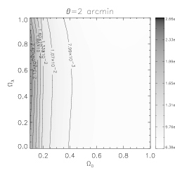
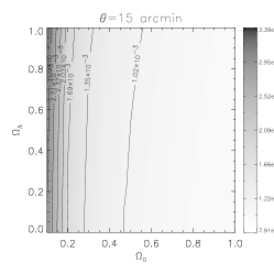
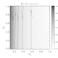
Figure 2: The dependence of $w_{\kappa\delta}$ on $\Omega_{0}$ and $\Omega_{\Lambda}$ is shown for two different angular scales ($\theta=2^{\prime}$, $15^{\prime}$ and $40^{\prime}$). Here we have used a cluster normalised cosmology, with $\Gamma=\Omega_{0}\,h$ and $\bar{b}=1$. On scales greater than one arc minute, the $\Omega_{\Lambda}$-dependence is so weak that this parameter can safely be eliminated.

3.3 Dependence on $\Omega_{0}$ and $\sigma_{8}$

Regarding the dependence of $w_{\kappa\delta}$ on $\Omega_{0}$ and $\sigma_{8}$, a rough inspection of Eq. (6) would give $w_{\kappa\delta}\propto\Omega_{0}\,\sigma_{8}^{2}$, where the factor $\Omega_{0}$ comes from Poisson’s equation, and the scaling $\propto\sigma_{8}^{2}$ reflects the normalisation of the power spectrum. However, closer examination reveals a more complicated dependence. Due to the nonlinear evolution of the power spectrum, $\sigma_{8}$ does not only change the correlation amplitude, but also its shape. Similarly, $\Omega_{0}$ affects the nonlinear evolution of the power spectrum, and therefore also changes the shape of $w_{\kappa\delta}$.

Figure 3 illustrates the dependence of $w_{\kappa\delta}$ on $\Omega_{0}$ and $\sigma_{8}$, at three angular scales, for fixed values of $h$ and $\bar{b}_{\mathrm{R}}$. For measurements taken at a single angular scale only, the dependence on $\Omega_{0}$ and $\sigma_{8}$ is degenerate. At small angular scales, for instance, an increase in $\Omega_{0}$ can be compensated by a decrease in $\sigma_{8}$ (cf. the left panel of Fig. 3). However, this degeneracy can be broken if measurements at different angular scales are combined. At large angular scales, for example, an increase in $\Omega_{0}$ would have to be compensated by an increase in $\sigma_{8}$ (cf. the right panel of Fig. 3). Therefore, the shape of the correlation function contains cosmological information, and it is thus important to measure the correlation signal across a wide range of angular scales. The dashed line in Fig. 3 shows the cluster normalisation constraint given by Eke et al. (1996).

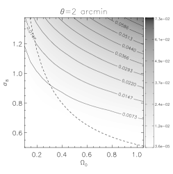
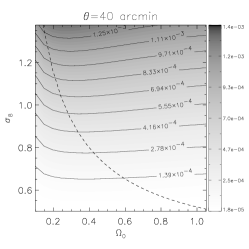
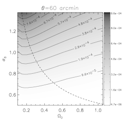
Figure 3: The dependence of $w_{\kappa\delta}$ on $\Omega_{0}$ and $\sigma_{8}$ is shown for three different angular scales ($\theta=2^{\prime}$, $40^{\prime}$ and $60^{\prime}$ from left to right) and assuming $\Gamma=\Omega_{0}\,h$. We kept $h=0.72$ and $\bar{b}=1$ fixed for the plot. As the dependence on $\sigma_{8}$ and $\Omega_{0}$ changes with angular scale, the degeneracy between these two parameters can be broken. At $\sim 40^{\prime}$, the correlation function is almost insensitive to $\Omega_{0}$. The dashed line shows the cluster normalisation from Eke et al. (1996).

We note that there is an interesting angular scale around $40^{\prime}$ where the quasar-galaxy cross-correlation function becomes almost independent of $\Omega_{0}$. The dependence of $w_{\kappa\delta}$ on $\Omega_{0}$ and $\sigma_{8}$ can be understood as follows:

• From Eq. (6), we see that the correlation function is roughly proportional to $\Omega_{0}\times\int s\mathrm{d}s\,P(s)\,\mathrm{J}_{0}(s\theta)$. At small angular scales, the Bessel function is close to unity over a large range of wave numbers $s$, and the result of the integration over $s$ is roughly proportional to $\sigma_{8}^{2}$. Hence, we have $w\propto\Omega_{0}\,\sigma_{8}^{2}$, whatever the value of $\Gamma$.

• At large angular scales, the oscillations of the Bessel function largely cancel the power at high wavenumbers, and thus the $s$ integration is only sensitive to the low-$s$ part of the power spectrum. Since this rising part of the power spectrum decreases rapidly with increasing $\Gamma$ (or equivalently increasing $\Omega_{0}$) and keeping the normalisation constraint fixed, the correlation amplitude decreases as $\Omega_{0}$ increases.

• At intermediate angular scales, the various effects of changing $\Omega_{0}$ cancel each other almost exactly, which leads to the insensitivity of the correlation amplitude to $\Omega_{0}$ at angular scales around $40^{\prime}$.

The overall dependence of $w_{\kappa\delta}$ on $\sigma_{8}$ and $\Omega_{0}$ reflects the physically motivated proportionality $\Gamma\propto\Omega_{0}$, which is the simplest possible relation between these parameters. More general cases will be taken into account in Sect. 4.3.

Our main conclusions from this section are that the dependence of $w_{\kappa\delta}$ on $\Omega_{\Lambda}$ is so weak that it can be neglected, and the degeneracy between $\sigma_{8}$ and $\Omega_{0}$ can be broken by measuring $w_{\kappa\delta}$ over a wide range of angular scales between a few arc minutes and one degree. Assuming $\Gamma=\Omega_{0}\,h$, $w_{\kappa\delta}$ becomes almost independent of $\Omega_{0}$ for angular scales near $40^{\prime}$. At that scale, the amplitude of the correlation function is proportional to $\bar{b}\,\sigma_{8}^{2}$, and a measurement of this product is in principle possible. We will address this point in Sect. 4.2.

4 Expected measurements

We now evaluate how accurately the remaining cosmological parameters can be constrained through measurements of quasar-galaxy cross-correlation functions. For that purpose, we simulate observations of quasar-galaxy cross-correlations expected to be possible with the Sloan Digital Sky Survey data.

4.1 Signal-to-noise estimate

Since our goal is to constrain cosmological parameters from quasar-galaxy cross-correlations, we now assess a strategy for optimally using the data. Within narrow, ring-shaped bins of radius $\theta$ centred on $N_{\mathrm{Q}}$ background QSOs, the total deviation of the galaxy count from its mean is

$$\sum_{i=1}^{N_{\mathrm{Q}}}\left(N_{\mathrm{G},i}-\bar{N}_{\mathrm{G}}\right)\approx N_{\mathrm{Q}}\,\bar{N}_{\mathrm{G}}\,w_{\mathrm{Q}G}(\theta)\;,$$ (9)

where $\bar{N}_{\mathrm{G}}$ is the mean galaxy count obtained from randomly selected fields, and $N_{\mathrm{G},i}$ the galaxy count in the ring centred on the $i$-th QSO. In a stack of such narrow, ring-shaped bins, the signal-to-noise ratio of the detection will be

$$\left(\frac{S}{N}\right)\approx\sqrt{N_{\mathrm{Q}}\,\bar{N}_{\mathrm{G}}}\,w_{\mathrm{QG}}(\theta)\;.$$ (10)

As we saw before, the quasar-galaxy cross-correlation function $w_{\mathrm{QG}}(\theta)$ is larger than the cross correlation $w_{\kappa\delta}$ between convergence and projected density contrast by a factor $2\,(\alpha-1)\,\bar{b}$. The value of the bias factor $\bar{b}_{\mathrm{R}}$ is expected from simulations fall near unity. However, the value of $(\alpha-1)$ depends on the quasar sample.

The measured cumulative quasar number-count function strongly depends on the selection criteria of the quasars. For our measurement, we first need a cut at low redshift to exclude any overlap between the QSOs and the galaxies. Then, for a given magnitude range, we need a clean and complete sample. Since most of the SDSS quasars are photometric, this implies cutting the sample in multicolour space for optimising the selection criteria. We leave this level of detail aside in this paper. We use the fitting function provided by Pei (1995) for estimating the cumulative quasar number-counts as a function of magnitude, i.e. a broken power law with slopes of $\alpha\sim 0.64$ for QSOs fainter than $B\sim 19$, and $\alpha\sim 2.52$ for brighter QSOs.

Since faint QSOs have $\alpha<1$, they are negatively-biased by the lensing magnification. Thus, taking all observed QSOs straightforwardly into account would tend to reduce or even reverse the correlation signal. However, we can separate the dependences of $w_{\mathrm{QG}}(\theta)$ on angular scale (which contains the cosmological information) and on quasar magnitude and thus keep all information required to stack the correlation signal from all quasars in a sample.

The Cauchy-Schwarz inequality provides optimal weights for quasars with respect to magnitude. We find that the signal-to-noise ratio is optimised by

$$\left(\frac{S}{N}\right)_{\rm opt} \approx \frac{\int\mathrm{d}m\,(\alpha(m)-1)^{2}\,N_{Q}(m)}{\int\mathrm{d}m\,|\alpha(m)-1|\,\sqrt{N_{Q}(m)}}\,\sqrt{\bar{N}_{G}}\;2\,\bar{b}_{\mathrm{R}}\,w_{\kappa\delta}(\theta)\;,$$

where $N_{\mathrm{Q}}(m)$ is the number of quasars in the magnitude bin $[m,m+\mathrm{d}m]$, and $\alpha(m)$ is the corresponding slope of the number counts. Therefore, we can consider the following effective correlation function

$$w_{\mathrm{eff}}(\theta)=2\,\bar{b}_{\mathrm{R}}\,(\alpha_{\mathrm{eff}}-1)\,w_{\kappa\delta}(\theta)\;,$$ (11)

where $\alpha_{\mathrm{eff}}$ is an effective slope describing the entire quasar sample,

$$\alpha_{\mathrm{eff}}=1+\frac{1}{\sqrt{N_{Q}}}\frac{\int\mathrm{d}m\,(\alpha(m)-1)^{2}\,N_{Q}(m)}{\int\mathrm{d}m\,|\alpha(m)-1|\,\sqrt{N_{Q}(m)}}\;.$$ (12)

The signal-to-noise ratio of the optimally weighted data can now simply be calculated using $w_{\mathrm{eff}}$ instead of $w_{\mathrm{QG}}$ in Eq. (10). The effective correlation function $w_{\mathrm{eff}}(\theta)$ is related to an average absolute deviation of the galaxy number counts in the vicinity of quasars from their mean, weighted appropriately. In effect, each magnitude bin gives a constructive signal to the cross-correlation, and the weighting ensures a maximised signal-to-noise ratio. To get an idea of a reasonable value for $\alpha_{\mathrm{eff}}$, we use Pei’s (1995) broken power-law fit for a sample of QSOs ranging in magnitude from $m=16$ to $m=21$. Evaluating the integral in Eq. (4.1), we find that $\alpha_{\mathrm{eff}}=1.35$.

Some quasars have a magnitude $m$ for which $|\alpha(m)-1|\approx 0$, so they will only contribute noise to the final correlation function. Those quasars are down-weighted by Eq. (4.1), but the selection can be further restricted by keeping only quasars whose signal-to-noise ratio for the lensing effect exceeds a specified threshold. The sample is then constrained by the condition

$$|\alpha(m)-1|>\frac{1}{\sqrt{N_{\mathrm{Q}}\,\bar{N}_{\mathrm{G}}}\,2\,\bar{b}_{\mathrm{R}}\,w_{\kappa\delta}(\theta)}\;.$$ (13)

The number of quasars satisfying this criterion is expected to be a large fraction of the total available sample. We thus neglect the sample restriction in the following, but it should be taken into account in any measurement of $w_{\mathrm{QG}}$ from real data.

In the previous section, we emphasised the importance of measuring the cross-correlation across a wide range of angular scales with a good signal-to-noise ratio. Thus, the size of the ring-shaped bins around quasars in which galaxies are counted must change with the ring radius $\theta$. At large radii, wide bins are needed, and the earlier narrow-bin calculation no longer holds. The general result for an annular bin is

$$\left(\frac{S}{N}\right)=\sqrt{\bar{n}_{\mathrm{G}}\,N_{\mathrm{Q}}}\,\frac{\int\mathrm{d}^{2}\phi\,w_{\mathrm{eff}}(\phi)\,[U_{\theta^{\prime}}(\phi)-U_{\theta}(\phi)]}{\sqrt{\pi(\theta^{\prime 2}-\theta^{2})}}\;,$$ (14)

where $U_{\theta}$ is a top-hat filter of radius $\theta$. This integration over a disk replaces the zeroth-order Bessel function $\mathrm{J}_{0}(s\theta)$ in Eq. (6) by $2\pi\theta\mathrm{J}_{1}(s\theta)/s$, and thus

$$\int\mathrm{d}^{2}\phi\,w_{\kappa\delta}(\phi)\,U_{\theta}(\phi) = \int\mathrm{d}w\,\frac{p_{\kappa}(w)\,p_{\delta}(w)}{f_{K}^{2}(w)}$$

$$\times \int\mathrm{d}s\,P_{\delta}\left(\frac{s}{f_{K}(w)},w\right)\,\theta\,\mathrm{J}_{1}(s\theta)\;.$$

In order to adapt this model to a forthcoming application to the SDSS data sample, we will use the following parameters:

• The galaxy density is $\bar{n}_{\mathrm{G}}\simeq 3\,\mbox{arcmin}^{-2}$ (Scranton et al. 2001) for SDSS galaxies down to $r^{\prime}=22$. It is shown that masking of stars or bad seeing is important at that magnitude limit, and the usable area of the survey is reduced by a factor 2/3.

• The angular coverage is taken from $\theta=0.5^{\prime}$ to $1^{\circ}$ and separated in 15 logarithmically spaced bins. Below $0.5^{\prime}$, the shot noise becomes important due to the fairly low galaxy number density. Above one degree, the amplitude of the correlation function drops rapidly as shown in Fig. 1, and so does the signal of the galaxy overdensity.

• The effective logarithmic slope of the quasar number-count function is set to $\alpha_{\mathrm{eff}}=1.35$.

• The quasar number $N_{\mathrm{Q}}$ is essential for determining the signal-to-noise ratio. Its value is continuously increasing with the size of the survey and will reach its maximum in 2005. The SDSS Early Data Release contains approximately 4000 spectroscopic quasars and 9000 quasar candidates based on photometry alone. The expected quasar number of the final survey is on the order of $10^{5}$ for spectroscopically identified quasars, and can reach on the order of $10^{6}$ for photometrically selected quasars (G. Richards, private communication). Furthermore, we need a quasar sample which is well separated in redshift from the galaxy sample. For this purpose, we will only use quasars with $z\geq 1$. In order to account for these numbers and for the reduction of the usable survey area due to masking, we will consider an effective number of quasars $N_{\mathrm{Q}}$ between $5\times 10^{3}$ and $5\times 10^{5}$.

  Photometric redshifts will be available for all quasars. The amplitude of $w_{\mathrm{QG}}$ is mainly sensitive to the mean redshift of the considered quasar sample rather than its exact redshift distribution. Therefore we can safely neglect any uncertainties in the redshift estimates.

4.2 Constraints on $\bar{b}(40^{\prime})\,\sigma_{8}^{2}$

We saw earlier that assuming $\Gamma=\Omega_{0}\,h$ (or similar relations) causes the quasar-galaxy cross-correlation to be only weakly sensitive to $\Omega_{0}$ near the angular scale of $\sim 40^{\prime}$ (corresponding to an effective scale of roughly $8\,{\rm h}^{-1}_{50}\,{\rm Mpc}$), and this property can in principle be used to further reduce the parameter space. At angular scales near $40^{\prime}$, the density perturbations probed by the correlation function are well within the linear regime, where the amplitude of the power spectrum simply scales $\propto\sigma_{8}^{2}$. At that scale, the correlation amplitude scales $\propto b(40^{\prime})\,\sigma_{8}^{2}$ to good accuracy, almost independently of the density parameter $\Omega_{0}$ and the cosmological constant $\Omega_{\Lambda}$. Given $\Omega_{0}$, the shape parameter of the power spectrum is fixed by the Hubble constant. The product $\bar{b}(40^{\prime})\,\sigma_{8}^{2}$ can therefore be determined through the correlation amplitude only up to the level of uncertainty reflecting the uncertainty of the Hubble constant, and by the remaining weak dependence on $\Omega_{0}$. Figure 4 shows how the amplitude of the quasar-galaxy cross-correlation function near $40^{\prime}$ changes with the Hubble constant and the density parameter $\Omega_{0}$. The overall uncertainty is on the order of $20\%$.

Figure 4: $w_{\kappa\delta}(\Omega_{0};\theta=40^{\prime})$ is plotted for different values of $\Gamma$. The solid line is for $\Gamma=\Omega_{0}\,h$ with $h=0.72$, and the two dashed line are for $h=0.64$ and $h=0.80$, which are the 1-$\sigma$ confidence limits given by the Hubble Key Project. Here we have used $\sigma_{8}=1$.

The variation of $w_{\kappa\delta}$ with $\Omega_{0}$ can be reduced by narrowing the angular range from which the data are taken, however at the expense of the signal-to-noise ratio. Within an annulus with inner radius $30^{\prime}$ and outer radius $50^{\prime}$, where the amplitude of $w_{\mathrm{QG}}(\Omega_{0})$ changes by less than about $20\%$, the expected signal-to-noise ratio can be determined from Eq. (14) with the appropriate top-hat filters,

$$\left(\frac{S}{N}\right) = \sqrt{\bar{n}_{\mathrm{G}}\,N_{\mathrm{Q}}}\,\frac{\int\mathrm{d}^{2}\phi\,w_{\mathrm{eff}}(\phi)\,[U_{50^{\prime}}(\phi)-U_{30^{\prime}}(\phi)]}{\sqrt{\pi(50^{\prime 2}-30^{\prime 2})}}$$ (16)

$$\simeq 9\,\left(\frac{N_{Q}}{10^{5}}\right)^{1/2}\,\left(\frac{\bar{n}_{\mathrm{G}}}{3}\right)^{1/2}\,\left(\frac{2(\alpha_{\mathrm{eff}}-1)\,b(40^{\prime})}{0.7}\right)\;,$$

where we have used the number of spectroscopic quasars expected to be provided by the SDSS. Using photometric quasars, this signal-to-noise ratio might be improved. Therefore, the accuracy of a measurement of $\bar{b}(40^{\prime})\,\sigma_{8}^{2}$ through quasar-galaxy cross-correlations is limited by the uncertainties in the Hubble constant and the density parameter if $\Omega_{0}$ is treated as unknown. We emphasise the fact that the only external information we use for this method is the Hubble constant. Any additional constraint on $\Omega_{0}$ can substantially increase the precision of the $\bar{b}(40^{\prime})\,\sigma_{8}^{2}$ measurement.

4.3 Parameter estimates: $\Omega_{0}$, $\sigma_{8}$ and $\bar{b}_{\mathrm{R}}$

Figure 5: Expected constraints on the parameters $\Omega_{0}$ and $\bar{b}$ for cluster normalised universes. The input parameters used to create the simulated observation are $(\Omega_{0},\Omega_{\Lambda},\sigma_{8},\Gamma)=(0.3,0.7,1.0,0.21)$, and the bias was set to unity. The panels show the 1-, 2- and 3-$\sigma$ confidence levels for quasar sample sizes of $10^{4}$, $10^{5}$, using the relation $\Gamma=\Omega_{0}\,h$. The symbol ”$+$” shows the location of the input model, and the symbol ”$\times$” shows the minimum of the $\chi^{2}$.

Figure 6: Expected constraints on cosmological parameters. The contours show the 68%, 90%, and 95% confidence levels. The two panels show results for quasar sample sizes of $10^{4}$, $10^{5}$. The parameters of the input model are $(\Omega_{0},\Omega_{\Lambda},\sigma_{8},\Gamma)=(0.3,0.7,1.0,0.21)$, and $\bar{b}_{\mathrm{R}}=1$.

We now investigate possible parameter estimates using the information coming from all angular scales. Using Eqs. (14) and (4.1), we can simulate measurements of $w_{\mathrm{QG}}(\theta)$ and then compute the uncertainty of the parameter constraints we wish to extract from the data.

We saw above that the shape of the correlation function contains important information on the cosmological parameters. For achieving similar signal-to-noise ratios in all annular bins of the measurement, we use logarithmically spaced annuli around the quasars. In order to estimate the uncertainty of our parameters, it is worth noticing that $10^{5}$ quasars spread evenly across the whole survey area are on average separated by about $20^{\prime}$. Given our 15 logarithmically spaced bins covering the angular range introduced above, this means that the errors in the three outer bins would be effectively correlated. The others are only very weakly affected by possible correlations. Given the low amplitude of the cross-correlation, the Poisson noise dominates in our case. Hence, a simple $\chi^{2}$ of the difference between the simulated data and the model enables us to reasonably estimate the uncertainty of the parameters. However, it has to be kept in mind that we are ignoring any angular variation in the bias, which might contribute to the parameter uncertainties.

However, due to the large parameter space and some partial parameter degeneracies, the $\chi^{2}$ minimisation yields allowed ranges for the complete parameter set which are fairly wide compared to the existing parameter constraints. An attempt to find constraints on the full parameter space $(\Omega_{0},\sigma_{8},\Omega_{\Lambda},h,\bar{b}_{\mathrm{R}})$ is therefore not promising. We have to include additional information for better constraining our parameter set.

The prime advantage of the quasar-galaxy cross-correlations compared to other methods for estimating the cosmological parameters is its direct sensitivity to the galaxy bias factor. In addition, it is a weak-lensing based method which can directly measure $\Omega_{0}$ and provide an independent cross-check of results obtained from weak-shear observations, as it does not rely on the assumption of intrinsically uncorrelated galaxy ellipticities. The most accurate measurements of $\Omega_{0}$ will be provided by CMB experiments. They rely on information coming from photons emitted at the recombination epoch ($z\sim 1200$) and depend on the curvature of photon trajectories as they propagate through the Universe. An independent measurement of $\Omega_{0}$ using only low-redshift information probes the consistency of the cosmological model.

For the following, we will use two external pieces of information. The first is an estimate of the power spectrum normalisation $\sigma_{8}$. For this, we use the cluster normalisation relation: $\sigma_{8}=0.52\,\Omega_{0}^{-0.52+0.13\,\Omega_{0}}$ (Eke et al. 1996), since there is no precise and direct measurement of $\sigma_{8}$. The second is an estimate of the peak location of the power spectrum $\Gamma$. We will use either a direct measurement, provided by galaxy surveys, or a measurement of the Hubble constant $h$, if we adopt the relation $\Gamma=\Omega_{0}\,h$. Finally, the remaining unknown parameters of the problem are the density parameter $\Omega_{0}$, the density parameter corresponding to the cosmological constant $\Omega_{\Lambda}$, and the bias parameter $\bar{b}_{\mathrm{R}}$, of which $\Omega_{\Lambda}$ can be ignored.

Other reductions of the parameter space are of course possible, but this one is particularly attractive because it allows a measurement of the galaxy bias and its dependences on scale, galaxy morphology, magnitude etc. In what follows, our first fiducial model has $\Gamma=\Omega_{0}\,h$, $h=0.72$, in agreement with recent constraints from the Hubble Key Project (Freedman et al. 2001), and is cluster normalised. We will later drop this relation between $\Gamma$ and $\Omega_{0}$. Hence, we compute

$$\chi^{2}(\Omega_{0},b)=\sum_{i}\frac{\left[\delta N_{\mathrm{M}}(\theta_{i};\Omega_{0},\bar{b}_{\mathrm{R}})-\delta N_{\mathrm{obs}}(\theta_{i};\Omega_{0},\bar{b}_{\mathrm{R,0}})\right]^{2}}{\sigma_{i}^{2}}\;,$$ (17)

where $\delta N_{\mathrm{M}}(\theta_{i})$ and $\delta N_{\mathrm{obs}}(\theta_{i})$ are the overdensities of galaxies in bin number $i$ expected in the model and detected in the simulated observation, respectively, and $\sigma_{i}$ is the Poisson noise in that bin.

The results are shown in Fig. 5. For this example, we have assumed a cosmological model with $\Omega_{0}=0.3$, $\Omega_{\Lambda}=0.7$ and a galaxy bias factor of unity. The contours show the 68.3%, 95.5%, and 99.7% confidence levels. Results for two different quasar sample sizes are presented, namely $10^{4}$ and $10^{5}$ quasars, from left to right. We see that a large quasar sample is required in order to at least confirm a low $\Omega_{0}$.

Previous quasar surveys listed only a few thousand objects, therefore we expect the SDSS to provide us with the first quasar-galaxy cross-correlation measurement with a reasonable signal-to-noise ratio that allows the extraction of some cosmological information. The two contour plots show a near-degeneracy between $\Omega_{0}$ and $\bar{b}_{\mathrm{R}}$, for low $\Omega_{0}$. Indeed, by lowering $\Omega_{0}$ the correlation function increases due to the cluster normalisation. For low $\Omega_{0}$, mainly the amplitude of the correlation function changes rather than its shape. Low values of the bias parameter can compensate for this change and still allow a good fit. Thus, assuming the relation $\Gamma=\Omega_{0}\,h$, quasar-galaxy correlations can provide an estimate of $\Omega_{0}$, but only poorly constrain $\bar{b}_{\mathrm{R}}$. Figure 5 also shows that $\bar{b}$ can be measured with good accuracy if the cosmological parameters are assumed to be known; $\Delta\bar{b}_{\mathrm{R}}\approx 15\%$ for $\Omega_{0}=0.3$.

As we discussed before, it is possible to probe other parameters with the quasar-galaxy cross-correlation function. For example, Fig. 6 shows what confidence intervals we can expect for $\Omega_{0}$ and $\sigma_{8}$, assuming $h=0.72$ and $\bar{b}_{\mathrm{R}}=1$. For instance, an independent measurement of the bias can be obtained combining cosmic shear and galaxy counts provided similar galaxy samples are considered (cf. Schneider 1998 and van Waerbeke 1998 for the theory, and Hoekstra et al. 2001b, in preparation, for a measurement using a joint analyses of the Red Cluster Survey and the VIRMOS-DESCART Survey). Using external information on $\bar{b}_{\mathrm{R}}$, we see that interesting constraints on $\Omega_{0}$ and $\sigma_{8}$ can be derived: we find $\Delta\Omega_{0}\sim 10\%$ and $\Delta\sigma_{8}\sim 5\%$.

Figure 7: Expected constraints on cosmological parameters. The contours show the 68%, 90%, and 95% confidence levels, for a quasar sample size of $10^{5}$, considering the fixed value $\Gamma=0.21$. The parameters of the input model are $(\Omega_{0},\Omega_{\Lambda},\sigma_{8},\Gamma)=(0.3,0.7,1.0,0.21)$, and $\bar{b}_{\mathrm{R}}=1$. The frame in the left panel shows how the 1-$\sigma$ contour moves by considering $\Gamma=0.21$, but having $\Gamma_{\mathrm{true}}=0.19$ or $0.23$.

The validity of the assumed relation $\Gamma=\Omega_{0}\,h$ (or more generalised relations taking baryons and neutrinos into account) depends on the matter and radiation content of the Universe, which is presently uncertain. For a more conservative approach, one can drop this relation and use measurements for $\Gamma$. The two plots in Figure 7 show the corresponding changes of the confidence levels. In the $\Omega_{0}$-$\bar{b}_{\mathrm{R}}$ plane, we see that we then get interesting constraints of the parameters. As we can expect in the $\Omega_{0}$-$\sigma_{8}$ plane, the contours are not significantly affected, and an interesting sensitivity on $\Omega_{0}$ and $\sigma_{8}$ remains. Similar contour plots can be obtained from cosmic-shear measurements (e.g. Van Waerbeke et al. 2001) by assuming a fixed value for $\Gamma$. As shown in Figure 7, quasar-galaxy cross-correlations measured with the SDSS will soon enable us to probe these parameters equally well as cosmic shear does with current deep imaging surveys.

Regarding $\Omega_{0}$ and $\bar{b}_{\mathrm{R}}$, we saw from the different contour plots that we achieve much higher sensitivity by using external information on $\Gamma$. Table 1 summarises the uncertainties on $\Omega_{0}$ and $\bar{b}_{\mathrm{R}}$ we can achieve, depending on the quasar sample size. We can reasonably expect the final usable quasar number to be at least of the order of $10^{5}$, which means an independent measurement of $\Omega_{0}$ with an accuracy of $\sim 17\%$, and of $\bar{b}_{\mathrm{R}}$ with an accuracy of $\sim 10\%$, should be feasible.
Clearly, the final goal of using quasar-galaxy correlations is probing the galaxy bias, but as these plots show, this method can also be used for constraining cosmological parameters.

effective quasar number	$\Delta\Omega_{0}$	$\Delta\bar{b}_{\mathrm{R}}$
$1\times 10^{4}$	$0.14$	$0.25$
$5\times 10^{4}$	$0.07$	$0.12$
$1\times 10^{5}$	$0.05$	$0.09$

Table 1: 1-$\sigma$ uncertainties expected for $\Omega_{0}$ and $\bar{b}_{\mathrm{R}}$ as functions of the effective quasar number, using SDSS parameters and the input values $\Omega_{0}=0.3$ and $\bar{b}_{\mathrm{R}}=1$. Here, we consider a cluster normalised $\Lambda$CDM cosmology and a fixed value for $\Gamma$.

The additional parameter $\Gamma$ is now known to approximately $20\%$ (Dodelson et al. 2001), and its accuracy is expected to greatly improve with SDSS in the near future. However, this uncertainty adds to the uncertainty of $\Omega_{0}$ and $\bar{b}_{\mathrm{R}}$. To see the implications, the frame in the left panel of Fig. 7 shows the effect on the 1-$\sigma$ confidence level of using different values of $\Gamma$. The dashed line represents the 1-$\sigma$ contour computed for the correct value of $\Gamma$ used for the simulations ($\Gamma=0.21$); the upper and lower contours are computed for $\Gamma=0.23$ and $\Gamma=0.19$, respectively. From this plot, we can see that mistaking $\Gamma$ by $10\%$ will introduce a systematic of about $16\%$ in $\bar{b}_{\mathrm{R}}$ and $10\%$ in $\Omega_{0}$.

5 Conclusion and prospects

Background quasars and foreground galaxies are cross-correlated on angular scales between $\sim 1^{\prime}$ and $\sim 1^{\circ}$ through the magnification bias due to weak lensing by large-scale structures. The effect probes the dark matter distribution in the Universe in much the same way as measurements of cosmic shear do, but by counting objects instead of measuring shapes, and thus without the crucial assumption that the ellipticities of background galaxies are uncorrelated. In addition, the lensing-induced QSO-galaxy correlations probe the relation between the distributions of galaxies and dark matter.

The existence of statistically significant correlations between foreground galaxies and background quasars has firmly been established. Up to now, however, the quasar-galaxy correlation function $w_{\mathrm{QG}}$ could not be reliably measured because homogeneous, sufficiently deep, wide-field galaxy surveys were missing. With the advent of such surveys, for which the Sloan Digital Sky Survey (SDSS) is the prototypical example, a measurement of this weak lensing effect with high signal-to-noise ratio is now within reach.

Using quasar-galaxy cross-correlations and assuming a linear and deterministic bias, Benítez & Sanz (2000) showed how to measure $\Omega_{0}/\bar{b}$ at a given angular scale from the ratio $w_{\mathrm{QG}}(\theta)/w_{\mathrm{GG}}(\theta)$ between the quasar-galaxy cross-correlation and the galaxy-galaxy autocorrelation functions. However, their method discards the information contained in the amplitude and angular shape of $w_{\mathrm{QG}}$. In this paper, we investigated what kind of cosmological information can be expected from an accurate measurement of $w_{\mathrm{QG}}$ using the SDSS data. Our main assumptions were that

• galaxies are biased relative to the dark matter, possibly in a non-linear or stochastic way.

• the shape parameter of the power spectrum either satisfies $\Gamma\propto\Omega_{0}\,h$, or can be fixed by the peak location in galaxy power spectra;

• the power spectrum is normalised such that the local abundance of rich galaxy clusters is reproduced; and

• the lensing magnification is weak. $|\mu-1|\ll 1$.

Under these assumptions, $w_{\mathrm{QG}}$ depends in principle on the density parameter $\Omega_{0}$, the cosmological constant $\Omega_{\Lambda}$, the Hubble constant $h$ (or $\Gamma$), the normalisation of the power spectrum $\sigma_{8}$, and the bias parameter $\bar{b}$. This parameter range is too large to allow any accurate cosmological constraints from the quasar-galaxy correlations alone. However, the parameter range can safely be reduced. We showed that:

1. the dependence of the quasar-galaxy cross-correlation function on the cosmological constant $\Omega_{\Lambda}$ is entirely negligible on scales above one arc minute;

2. assuming the relation $\Gamma=\Omega_{0}\,h$, we find an interesting angular range within which the amplitude of $w_{\mathrm{QG}}$ is insensitive to $\Omega_{0}$, and where its amplitude is simply proportional to $\bar{b}(40^{\prime})\,\sigma_{8}^{2}$;

3. neglecting any relation between $\Gamma$ and the other parameters and using the cluster normalisation, the matter density and the bias parameter can be constrained with with $17\%$ and $10\%$ relative accuracy, respectively;

4. knowing the value of the bias parameter, it is possible to accurately measure of $\Omega_{0}$ and $\sigma_{8}$, namely with $17\%$ and $7\%$ relative accuracy, respectively.

We used a scale-independent bias, but models or measured constraints on $\bar{b}(\theta)$ can be included into the calculation of the cross-correlation function $w_{\mathrm{QG}}(\theta)$.

Our knowledge of the cosmological parameters will greatly improve over the next few years, partly through the wide-field galaxy surveys themselves, but most dramatically through the CMB experiments. Therefore, the quasar-galaxy cross-correlations will be less important for determinations of cosmological parameters, although they will allow important consistency checks. However, the most important contribution from a measurement of $w_{\mathrm{QG}}$ will be a direct determination of the galaxy bias factor on a broad range of scales, for different luminosities and morphological types of galaxies.

Williams & Irwin (1998) and Norman & Williams (2000) cross-correlated APM galaxies with LBQS and 1-Jansky quasars and claimed significant galaxy overdensities around quasars on angular scales of order one degree. As the amplitude of their correlations cannot be explained in terms of weak lensing by large-scale structures in a CDM universe, it is highly important to reexamine them.

Finally, the shape of $w_{\mathrm{QG}}$ depends on the shape of the underlying dark-matter power spectrum, and a measurement of $w_{\mathrm{QG}}$ will therefore test whether the CDM power spectrum adequately describes the weak-lensing effects by large-scale structure. This, of course, is also probed by cosmic shear, but only under the assumption that intrinsic galaxy ellipticities are uncorrelated. Measuring $w_{\mathrm{QG}}$ thus provides a useful, independent, weak-lensing based method for directly constraining the dark-matter power spectrum.

- (1) Bacon, D., Refregier, A., Ellis, R. S. 2000, MNRAS 318, 625
- (2) Bardeen, J. M., Bond, J. R., Kaiser, N.; Szalay, A. S., 1986, ApJ 304, 15
- (3) Bartelmann, M., 1995, A&A, 298, 661
- (4) Bartelmann, M. & Schneider, P., 1993, A&A, 271, 421
- (5) Bartelmann, M. & Schneider, P., 1994, A&A, 284, 1
- (6) Bartelmann, M., Schneider, P., & Hasinger, G., 1994, A&A, 290, 399
- (7) Bartelmann, M. & Schneider, P., 2001, Physics Reports 340, 291
- (8) Benítez, N., Martínez-González, E., 1995, ApJ 448, L89
- (9) Benítez, N., Sanz, 2000, ApJ 525, L1
- (10) Benítez, N., Sanz, J. L., Martínez-González, E., 2001, MNRAS 320, 241
- (11) Bernardeau, F., Van Waerbeke, L., Mellier, Y., 1997, A&A 322, 1
- (12) Dekel, A. & Lahav, O., 1999, ApJ, 520, 24
- (13) Dolag, K. & Bartelmann, M., 1997, MNRAS 291, 446
- (14) Dodelson, S., Narayanan V. K., Tegmark, M., Scranton, R., Budavari, T., Connolly, A., Csabai, I., Eisenstein, D., Frieman, J. A., Gunn, J. E., Hui, L., Jain, B., Johnston, D., Kent, S., Loveday, J., Nichol, R. C., O’Connell, L., Scoccimarro, R., Sheth, R. K., Stebbins, A., Strauss, M. A., Szalay, A. S., Szapudi, I., Vogeley, M. S., Zehavi, I., et al., for the SDSS Collaboration, astro/ph 0107421
- (15) Eke, V. R., Cole, S., Frenk, C. S., 1996, MNRAS 282, 263
- (16) Fugmann, W., 1990, A&A, 240, 11
- (17) Guimarães, A., C., C., van de Bruck, C., Brandenberger, R., H., 2001, MNRAS 325, 278
- (18) Freedman, W. L., Madore, B. F., Gibson, B. K., Ferrarese, L., Kelson, D. D., Sakai, S., Mould, J. R., Kennicutt, R. C. Jr., Ford, H. C., Graham, J. A., Huchra, J. P., Hughes, S. M. G., Illingworth, G. D., Macri, L. M., Stetson, P. B., 2001, ApJ 553, 47
- (19) Heavens, A., Refregier, A., Heymans, C. 2000, MNRAS 319, 649
- (20) Hoekstra, H., Franx, M., Kuijken, K., 2000, ApJ 532, 88
- (21) Hoekstra, H., Yee, H.K.C, Gladders, M., 2001a, astro-ph/0107413
- (22) Hoekstra, H., et al., 2001b, in preparation
- (23) Kaiser, N., Wilson, G., Luppino, G. A., 2000, astro-ph/0003338
- (24) Kauffmann, G., Colberg, J. M., Diaferio, A., White, S. D. M., 1999, MNRAS 307, 529
- (25) Norman, D. J. & Impey, C. D., 1999, AJ 118, 613
- (26) Norman, D. J. & Impey, C. D., 2001, ApJ 552, 473
- (27) Norman, D. J., Williams, L. L. R. 2000, AJ 119, 2060
- (28) Peacock, J.A, Dodds, S.J., 1996, MNRAS 280, L19
- (29) Pei, Y. C., 1995, ApJ 438, 623
- (30) Rodrigues-Williams, L. L. & Hogan, C. J., 1994, AJ, 107, 451
- (31) Sanz, J. L., Martínez-González, E., Benítez, N., 1997, MNRAS 291, 418
- (32) Schneider, P. 1998, ApJ 498, 43
- (33) Scranton, R., Johnston, D., Dodelson, S., Frieman, J. A., Connolly, A., Eisenstein, D. J., Gunn, J. E., Hui, L., Jain, B., Kent, S., Loveday, J., Narayanan, V., Nichol, R. C., O’Connell, L., Scoccimarro, R., Sheth, R. K., Stebbins, A., Strauss, M. A., Szalay, A. S., Szapudi, I.,Tegmark, M., Vogeley, M., Zehavi, I. & the SDSS Collaboration, 2001, astro-ph/0107416
- (34) Sugiyama, N., 1995, ApJS 100, 281
- (35) van Waerbeke, L. 1998, A&A 334, 1
- (36) van Waerbeke, L., Bernardeau, F., Mellier, Y., 1999, A&A 342, 15
- (37) van Waerbeke, L., Mellier, Y., Radovich, M., Bertin, E., Dantel-Fort, M., McCracken, H. J., Le Fèvre, O., Foucaud, S., Cuillandre, J.-C., Erben, T., Jain, B., Schneider, P., Bernardeau, F., Fort, B., 2001, A&A 374, 757
- (38) Williams, L. L. R., Irwin, M. 1998, MNRAS 298, 378
- (39) Wang, X., Tegmark, M., Zaldarriaga, M., 2001, astro-ph/0105091
- (40) Wittman, D. M., Tyson, J. A., Kirkman, D., Dell’Antonio, I., Berstein, G. 2000, Nature 405, 143
- (41) York, D. G., Adelman, J., Anderson, J. E., Anderson, S. F., et al. 2000, AJ, 120, 1607