Laminar plasma dynamos

Abstract

A new kind of dynamo utilizing flowing laboratory plasmas has been identified. Conversion of plasma kinetic energy to magnetic energy is verified numerically by kinematic dynamo simulations for magnetic Reynolds numbers above 210. As opposed to intrinsically-turbulent liquid-sodium dynamos, The proposed plasma dynamos correspond to laminar flow topology. Modest plasma parameters, 1–20 eV temperatures, $10^{19}$–$10^{20}$ m^-3 densities in 0.3–1.0 m scale-lengths driven by velocities on the order of the Alfvén Critical Ionization Velocity (CIV), self-consistently satisfy the conditions needed for the magnetic field amplication. Growth rates for the plasma dynamos are obtained numerically with different geometry and magnetic Reynolds numbers. Magnetic-field-free coaxial plasma guns can be used to sustain the plasma flow and the dynamo.

PACS numbers: 52.30.-q; 47.65.+a; 52.65.Kj; 52.72.+v

Dynamo action[1, 2] is believed to be the fundamental mechanism that creates the magnetic field commonly observed from planetary to galactic scales[3]. Conversion of kinetic (flow) energy into magnetic energy is the best known explanation for observed magnetic fields in the universe that are persistent against resistive diffusion. A direct experimental proof of the conversion of plasma flow energy to magnetic energy has not been accomplished to date. Another motivation of this letter is to show dynamo experiments can be performed in plasmas, as an alternative to liquid sodium or other conducting liquids[4]. The plasma dynamos discussed here are funadmentally different from what has generally been known for spheromaks[5, 6] and reversed field pinches[7, 8], when the term ‘dynamo’ has traditionally been invoked to explain conversion of one type of magnetic flux into another (toroidal flux into poloidal flux in the spheromak case). Because in these previous cases, the total magnetic field energy does not increase. In the present case, the plasma flow energy is converted into magnetic energy, and magnetic field is amplified accordingly.

Existing and proposed laboratory dynamo experiments [9, 10, 11] have used liquid sodium as conducting medium. Liquid sodium has low resistivity and viscosity[12] for conduction of electricity and fluid flow, as well as a low melting temperature which eases the creation of the liquid state for the conductor. A constraint on liquid sodium dynamos is intrinsically turbulent flow due to the small ratio of viscosity to resistivity[12]. The turbulent flow makes it difficult to make detailed comparisons between experiments and theories. Also, resistivity of the liquid sodium is only variable within a factor of two[10], which implies the magnetic Reynolds number, $Re_{m}$, may be varied only within a small range, primarily by variation of the experimental dimensions. Even with the high conductivity of the liquid sodium, existing technologies can only move liquid sodium at velocities no more than 20 m/sec[12]. Therefore $\sim$1 meter in size is necessary to have a dynamo excitation for a liquid sodium experiment, and $Re_{m}$ has been limited to values below a few hundred[10, 12].

Dynamo action is described by the induction equation[1, 2, 12]

$$\frac{\partial{\bf B}}{\partial t}=\nabla\times\left(\bf U\times{\bf B}\right)+\frac{\eta}{\mu_{0}}\nabla^{2}{\bf B},$$ (1)

where ${\bf U}$ is the fluid flow velocity, and $\eta$ is the resistivity. Without the flow U, the induction equation is a diffusion equation for magnetic field ${\bf B}$ with the characteristic diffusion time determined by the dimension of the field and resistivity. Only when U does not vanish may ${\bf B}$ grow by transfering the flow energy. The magnetic Reynolds number $Re_{m}\equiv\mu_{0}LU_{0}/\eta$ measures the relative amplitude of the flow drive to diffusion in Eq. (1), where $L$, $U_{0}$ and $\eta$ are characteristic values for the dimension, velocity field, and resistivity. Theories[12, 13] predict that only when the magnetic Reynolds number $Re_{m}$ exceeds certain threshold values (from 20 to 200, depending on the geometry), is dynamo action possible.

$Re_{m}$ greater than 200 appears easily achievable in flowing laboratory plasmas by this analysis. Thus an experiment is possible to create magnetic field energy that grows by transformation of the plasma flow energy alone. Such a new plasma dynamo can cover a wide range of magnetic Reynolds numbers both below and above the threshold by controlling the plasma flow velocity and the plasma resistivity. In the entire plasma system, one may encounter various length scales $L$, velocities $U$, as well as uncertain resistivity (the plasma resistivity is often ”anomalous”). Average, “global” values characteristic of the entire flow appear reasonable to use for comparison to theoretical threshold values of $Re_{m}$. In the plasma regime considered here where the flow is laminar (see below), the scale length $L$ is close to the dimension of the boundary. The characteristic velocity $U_{0}$ is representative of a Beltrami-flow profile[14], which is a flow satisfying $\nabla\times{\bf U}=\lambda_{B}{\bf U}$ with constant parameter $\lambda_{B}$. Spitzer resistivity provides a realistic estimate since the magnetic field is weak during the initial growth of the magnetic field, and the long plasma lifetimes imply local thermal equilibrium. In addition, energy balance is dominated by atomic physics (radiation by the electrons and boundary losses by the ions) and classical thermal conduction[15], and the plasma temperatures will be close to being in equilibrium and in the 1–20 eV range, even with substantial high-$Z$ impurities.

One key feature of these laboratory plasma dynamos is the high speed plasma flows (see Fig. 1) which will be on the order of the critical ionization velocity (CIV)[16]. CIV, denoted as $U_{c}$, is defined as $U_{c}\equiv\sqrt{2E_{i}/M_{i}}$, where $E_{i}$ is the ionization energy and $M_{i}$ the ion mass. A velocity of this magnitude is routinely achieved using plasma accelerators or thrusters[17]. For hydrogen gas, $U_{c}$ is 51 km/sec. For ease of estimation, the electron temperature determining the resistivity can be assumed to be in equilibrium with the ion temperature which is itself set to the “flow equivalent temperature” $T_{i}=(M_{i}U^{2})/2$. With this simplifying assumption, $Re_{m}$ scales as $Re_{m}=15T_{i}^{2}$[eV] $L$ [m]. For $L$ about 0.5 m and $T_{i}$ ranging from 1 to 20 eV, the $Re_{m}$ varies from 7.5 to 3000. The threshold $Re_{m}=200$ corresponds to $T_{i}=5.2$ eV, or a flow velocity of 31 km/sec for hydrogen, and hence in the expected range of CIV velocities. Because of the high plasma flow velocity, $Re_{m}$ in a plasma dynamo can be well above the threshold magnetic Reynolds number for magnetic field to grow, even considering that the resistivity of the plasma is much greater than that of liquid sodium. In Fig. 1, these plasma dynamos are compared with existing and proposed sodium dynamos, which are the only known laboratory dynamos so far.

Another unique feature of the new plasma dynamo is laminar flow. Flow topology is determined by the kinetic Reynolds number, $Re$, which characterizes the relative amplitude of the fluid convection to viscous dissipation in the Navier-Stokes equation. The critical Reynolds number for onset of turbulence $Re$ is more than a few thousand, and fluid motion is laminar for $Re$ below this threshold[18]. Plasmas discussed here can be approximated as fluids because the mean free path for particle motion is much less than the system dimension. The kinetic Reynolds number $Re$ then scales with the device dimension and plasma ion temperature as $Re=4.0\times 10^{-16}L$ [m] $n_{e}$ [m^-3]/$T_{i}^{2}$ [eV]. An experimental dimension $L$ of 0.5 m is adequate to meet the conditions of a plasma dynamo, with density 10¹⁹ to 10²⁰ m^-3 and temperature 1–20 eV. This corresponds to the kinetic Reynolds number $Re$ varying from 5 to 20000, which imply that plasma flow will be mostly laminar.

Plasma flow can be created using coaxial plasma guns, or Marshall guns[5, 19]. For the gun plasma momentum to be effectively transferred to the bulk plasma in a chamber, the mean free-path, $\lambda_{mfp}$, of the gun plasma ions should be less than the size of the dynamo chamber, that is, $\lambda_{mfp}<L$ is required. This is equivalent to $Re>2.5$, and hence the kinetic Reynolds number cannot be too small. The magnetic Prandtl number ($Pr_{m}$) is defined as the ratio $Pr_{m}=Re_{m}/Re$ and scales as $T_{i}^{4}/n_{e}$ with values in the range of 3.7$\times 10^{-4}$ to 600 for the plasma parameters above. In comparison, the $Pr_{m}$ for liquid sodium experiments is $\sim 10^{-5}$. The plasma Prandtl number can be very similar to that of the interior of the sun or the galactic plasma dynamos, albeit at very much lower Reynolds numbers.

The gun-plasma momentum transfer is also affected by ion-neutral collisions, which include ion-neutral momentum transfer and ion-neutral charge exchange. The ion-neutral momentum transfer cross section is 100 times less than that of ion-ion collision[20]. Therefore, as long as the ionization fraction is greater than 1%, ion-neutral momentum transfer can be neglected. The charge exchange cross section is about half of that of ion-ion momentum transfer. Therefore ion-ion momentum transfer is the dominant process for gun-plasma momentum transfer. Generation of toroidally rotating plasmas is most efficient when the ionization fraction is greater than 30%.

A possible experimental configurationtion is shown in Fig. 2, when one ‘main gun’ (Labeled as MG) is used together with three ‘toroidal guns’ (TG, not shown) to produce toroidal and poloidal plasma flows. Kinetic energy density for a 13 eV and 10¹⁹ m^-3 plasma is equivalent to a magnetic field strength of 53 gauss at the same energy density. Theoretical studies indicate that the fraction of the plasma flow kinetic energy that can be converted into magnetic field depends on the ratio of the magnetic Reynolds number to the kinetic Reynolds number[21]. As much as 20% of the flow energy was seen to convert into magnetic field numerically. If this is the case, magnetic field of up to 24 gauss may be generated when the back-reaction of the magnetic field on plasma flow is taken into account.

Numerical results confirm the existence of laminar plasma dynamos. The plasma flow is approximated by a Beltrami flow, $\nabla\times{\bf U}=\lambda_{B}{\bf U}$, which corresponds to a state of maximum kinetic helicity [$\int dV({\bf U}\cdot{\nabla\times{\bf U}})$] for a given total kinetic energy and a given boundary condition. We can use the Beltrami flow approximation because the flow is laminar here, large coherent flow pattern can be established. The Beltrami flow is also an eigenmode for the cylindrical boundary condition considered. Theoretical results indicate that large kinetic helicity content can lead to large dynamo growth rate. The solution of axisymmetric Beltrami flow inside the cylinder $0<r<R$ and $-L/2<z<L/2$ may be written in terms of a poloidal flux function $\Psi(r,z)$

$$\Psi=rJ_{1}\left(j_{11}\frac{r}{R}\right)\cos\frac{\pi z}{L}\mbox{,}$$ (2)

$$U_{r}=-\frac{1}{r}\frac{\partial\Psi}{\partial z}\mbox{,}\quad U_{z}=\frac{1}{r}\frac{\partial\Psi}{\partial r}\mbox{,}\quad U_{\phi}=\frac{\lambda_{B}\Psi}{r}$$ (3)

where $J_{1}(x)$ is a first order Bessel function in its standard notation, and $j_{11}$ is the first root of $J_{1}(x)=0$, $\lambda_{B}^{2}=j_{11}^{2}/R^{2}+\pi^{2}/L^{2}$. The velocity components $U_{r}$, $U_{z}$, and $U_{\phi}$ have been normalized to a characteristic velocity $U_{0}$.

The kinematic dynamo problem for Beltrami flows satisfying Eqs. (2) and (3) is implemented numerically as follows. The flow field is taken as given and the back reaction of the growing magnetic field on the flow is neglected. This approximation is justified for the initial stage of the exponential dynamo growth, when the magnetic field is weak and does not influence the flow. Instead of solving the induction equation Eq. (1) for ${\bf B}$ directly, potentials ${\bf A}$ and $\varphi$ are introduced. Using the gauge condition $\varphi-{\bf U}\cdot{\bf A}+(\eta/\mu_{0})\nabla\cdot{\bf A}=0$ [22], one can derive the following equation of evolution for the vector potential ${\bf A}$,

$$\frac{\partial A^{i}}{\partial t}=-A_{k}\frac{\partial U^{k}}{\partial x^{i}}-U^{k}\frac{\partial A^{i}}{\partial x^{k}}+\frac{\eta}{\mu_{0}}\frac{\partial^{2}A^{i}}{\partial x^{k}\partial x_{k}}\mbox{,}$$ (4)

where the resistivity $\eta$ is assumed to be constant throughout the cylinder and the coordinate notations refer to a Cartesian coordinate system $x^{i}$. A 3D kinematic dynamo code is used to solve Eq. (4). Then, the magnetic field can be obtained at any time by taking the curl of ${\bf A}$. The code is written for cylindrical coordinates, and it uses an explicit scheme with central spatial differencing in the advection term and standard nine points stencil for the diffusion term. Since the conductivity of metallic walls is much higher than the conductivity of the plasma, a perfectly conducting boundary is a good approximation. All boundaries of the cylinder ($r=R$, $z=-L/2$, and $z=L/2$) are assumed to be perfect conductors. Then, the boundary conditions for ${\bf A}$ at perfectly conducting boundaries compatible with the gauge can be chosen as follows: both the components of ${\bf A}$ parallel to the boundary and the divergence of ${\bf A}$ at the boundaries are zero. This gives three boundary conditions for three components of vector potential. Eq. (4) has a unique solution. A detailed description of the code, of the gauge choices, and of the implementation of the boundary conditions can be found in Ref. [23].

In the case of axisymmetric flow, the nonaxisymmetric modes of the magnetic field, which are proportional to $\exp(in\phi-i\omega t)$ with different azimuthal wavenumbers $n$ (also known as toroidal mode numbers), are decoupled from each other and are eigenmodes of Eq. (1) or Eq. (4). The 3D kinematic code picks up the fastest growing mode of the dynamo, which turns out to be the $n=1$ mode. Since the structure of each eignemode is two dimensional in $(r,z)$ coordinates, a 2D code involving only the azimuthal component of the magnetic field saves much time for simulations with varying boundary parameters. Such a 2D code for the vector potential evolution has also been written and used to calculate the dependencies of the growth rates of the $n=1$ mode on the boundary dimensions. The growth rates and the structure of the $n=1$ modes obtained using the 3D dode agree remarkably well with that using the 2D code. The modes have an oscillatory nature, i.e. the oscillation frequency $\omega=\omega^{\prime}+i\gamma(U_{max}/L)$ has real and imaginary parts, where both the rotation frequency $\omega^{\prime}$ and the dimensionless growth rate $\gamma$ are real. $U_{max}/L$ is about 100 kHz. $U_{max}$ is the maximum absolute velocity inside the cylinder. Exponentially growing (or decaying) magnetic fields also rotate with certain frequency, which comparable to the frequency of the fluid rotation, $\omega^{\prime}\sim 100$ kHz.

Dependence of the growth rate $\gamma$ on the magnetic Reynolds number $Re_{m}$ and on the aspect ratio $R/L$ of the cylinder is explored. Fig. 3a shows the dependence of $\gamma$ on $Re_{m}$ for a fixed aspect ratio $R/L=1$. Negative values of $\gamma$ correspond to decaying magnetic field. For $Re_{m}$ smaller than the threshold value of 210, the dynamo will not grow. With increasing $Re_{m}$, the growth rate first increases up to the maximum value $\sim 0.022$ (a growth time of 0.45 msec) at $Re_{m}=500$, and it subsequently decreases to smaller values but remains positive. Such behavior is typical for slow dynamos (for example, see Ref. [3]). Thus, these laminar plasma dynamos are slow dynamos, for which $\gamma$ asymptotically goes to zero for $Re_{m}\to\infty$. The laminar and regular (as opposed to chaotic) fluid motion stretches the magnetic field linearly in time. Exponential growth is only possible due to small diffusivity of the magnetic field, which recreates the component of the magnetic field perpendicular to the flow. When the diffusion of the magnetic field becomes very small ($R_{m}\rightarrow\infty$), the growth rate $\gamma$ also decreases to 0. Fig. 3b shows the dependence of $\gamma$ on the aspect ratio $R/L$ for a fixed $Re_{m}=500$. Dynamo does not exist for very long or very short cylinders. It is necessary to have comparable $R$ and $L$ for efficient excitation of the dynamo. In particular, at an experimentally feasible value of $Re_{m}=500$, the maximum growth rate $\gamma=0.055$ is achieved at $R/L=0.6$. These results suggest that a somewhat elongated cylindrical vessel will be the best for the excitation of dynamo. Pulsed plasma flow of several msec long should be sufficient to excite the laminar dynamos.

In conclusion, a theoretical study has shown dynamo can be excited to convert plasma kinetic energy into magnetic field energy in a laboratory environment. These plasma dynamos are laminar because of the low kinetic Reynolds number. Modest plasma parameters self-consistently satisfy the conditions needed for the dynamo. Numerical calculation yields a threshold magnetic Reynolds number of 210 for exponential growth of the laminar plasma dynamos in a cylindrical boundary with Beltrami flows. These results indicate that a new type of laboratory dynamo experiments is possible.

We thank Drs. Hui Li and Stirling Colgate for many useful suggestions to this work. One of us, VIP, would also like to thank Dr. John Finn for his advice on numerical simulations. This work is supported by U.S. DOE Contract No. W-7405-ENG-36. VIP acknowledges partial support from DOE grant DE-FG02-00ER54600

Figures

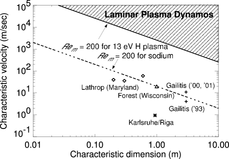
FIG. 1.:  Flow velocity vs experimental size for various sodium dynamos and for laminar plasma dynamos (Shaded region). Specific region of the laminar plasma dynamos may vary with gas species.

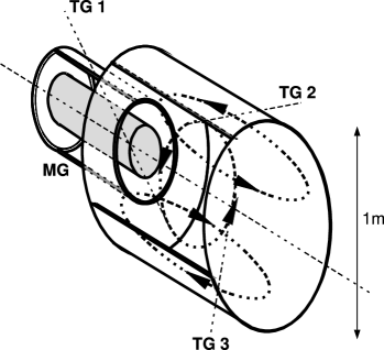
FIG. 2.:  A possible laminar plasma dynamo configuration using coaxial plasma guns.

FIG. 3.:  The dimensionless growth rate of the toroidal mode $n=1$ of a laminar plasma dynamo ($\gamma$) as a function of the magnetic Reynolds number, $Re_{m}$, for aspect ratio $R/L=1$.

FIG. 4.:  Dependence of the dimensionless growth rate of the toroidal mode $n=1$ of a laminar plasma dynamo ($\gamma$) on the aspect ratio, $R/L$, for fixed magnetic Reynolds number $Re_{m}=500$.

REFERENCES

- [1] H. K. Moffat, Magnetic Field Generation in Electrically Conducting Fluids, (Cambridge University Press, Cambridge, UK 1978).
- [2] R. M. Kulsrud, Annu. Rev. Astron. Astrophys. 37, 37 (1999).
- [3] See, for example, Ya B. Zeldovich, A. A. Ruzmaikin and D. D. Sokoloff, Magnetic Field in Astrophysics, Gordon & Breach, (London, 1983); P. H. Roberts, and A. M. Soward, Ann. Rev. Fluid Mech. 24, 459 (1992).
- [4] A. Tilgner, Phys. Earth Planet. Inter. 117, 171 (2000)
- [5] T. R. Jarboe, Plasma Phys. Control. Fusion 36, 945 (1994).
- [6] C. W. Barnes, J. C. Fernandez, I. Henins, et al., Phys. Fluids 29, 3415 (1986).
- [7] K. F. Schoenberg, R. W. Moses, and R. L. Hagenson, Phys. Fluids 27, 1671 (1984).
- [8] H. Ji, S. C. Prager, A. F. Almagri, J. S. Scarff, Y. Yagi, Y. Hirano, K. Hattori, and H. Toyama, Phys. Plasmas 3, 1935 (1996).
- [9] A. Gailitis, O. Lielausis, E. Platacis, S. Dement’ev, A. Cifersons, G. Gerbeth, T. Gundrum F. Stefani, M. Christen and G. Will, Phys. Rev. Lett. 86, 3024 (2001).
- [10] A. B. Reighard and M. R. Brown, Phys. Rev. Lett. 86, 2794 (2001).
- [11] N. L. Peffley, A. B.Cawthorne, D. P. Lathrop, Phys. Rev. E 61, 5287 (2000).
- [12] P. H. Roberts, and T. H. Jensen, Phys. Fluids B 5, 2657 (1992)
- [13] G. A. Glatzmaier and P. H. Roberts, Int. J. Eng. Sci. 36, 1325 (1998).
- [14] A. Kageyama and T. Sato, Phys. Plasmas 6, 771 (1999).
- [15] S. I. Braginskii, in Reviews of Plasma Physics, Vol. 1, (consultant Bureau, New York, 1965), p. 205.
- [16] N. Brenning, Space Sci. Rev. 59, 209 (1992).
- [17] K. F. Schoenberg, R. A. Gerwin, R. W. Moses, Jr. , J. T. Scheuer, and H. P. Wagner, Phys. Plasmas 5, 2090 (1998).
- [18] V. V. Vasilev and V. E. Strelnitskij, Diam. Related Mater. 8, 202 (1999).
- [19] Z. Wang and C. W. Barnes, Phys. Plasmas 8, 4218 (2001).
- [20] R. J. Goldston and P. H. Rutherford, Introduction to Plasma Physics, (IoP Publishing, Bristol, UK, 1995).
- [21] R. G. Kleva, and J. F. Drake, Phys. Plasmas 2, 4455 (1995).
- [22] V. I. Pariev, S. A. Colgate, and J. M. Finn, to submit to Astrophys. J. .
- [23] V. I. Pariev, Ph. D Thesis, University of Arizona (Tucson, 2001).