Gravitational Lensing of the SDSS High-Redshift Quasars

Abstract

We predict the effects of gravitational lensing on the color-selected flux-limited samples of $z_{\rm s}\sim 4.3$ and $z_{\rm s}\gtrsim 5.8$ quasars, recently published by the Sloan Digital Sky Survey (SDSS). Our main findings are: (i) The lensing probability should be 1–2 orders of magnitude higher than for conventional surveys. The expected fraction of multiply-imaged quasars is highly sensitive to redshift and the uncertain slope of the bright end of the luminosity function, $\beta_{h}$. For $\beta_{h}=2.58$ (3.43) we find that at $z_{\rm s}\sim 4.3$ and $i^{*}<20.0$ the fraction is $\sim 4\%$ ($13\%$) while at $z_{\rm s}\sim 6$ and $z^{*}<20.2$ the fraction is $\sim 7\%$ ($30\%$). (ii) The distribution of magnifications is heavily skewed; sources having the redshift and luminosity of the SDSS $z_{\rm s}\gtrsim 5.8$ quasars acquire median magnifications of $med(\mu_{obs})\sim 1.1$–$1.3$ and mean magnifications of $\langle\mu_{obs}\rangle\sim 5$–$50$. Estimates of the quasar luminosity density at high redshift must therefore filter out gravitationally-lensed sources. (iii) The flux in the Gunn-Peterson trough of the highest redshift ($z_{\rm s}=6.28$) quasar is known to be $f_{\lambda}<3\times 10^{-19}{\rm erg\,sec^{-1}\,cm^{-2}\AA^{-1}}$. Should this quasar be multiply imaged, we estimate a 40% chance that light from the lens galaxy would have contaminated the same part of the quasar spectrum with a higher flux. Hence, spectroscopic studies of the epoch of reionization need to account for the possibility that a lens galaxy, which boosts the quasar flux, also contaminates the Gunn-Peterson trough. (iv) Microlensing by stars should result in $\sim 1/3$ of multiply imaged quasars in the $z_{\rm s}\gtrsim 5.8$ catalog varying by more than 0.5 magnitudes over the next decade. The median emission-line equivalent width of multiply imaged quasars would be lowered by $\sim 20\%$ with respect to the intrinsic value due to differential magnification of the continuum and emission-line regions.

1 Introduction

The Sloan Digital Sky Survey (SDSS; Fukugita et al 1996; Gunn et al. 1998; York et al. 2001) has substantially increased the number of quasars known at a redshift $z_{\rm s}>3.5$ (Fan et al. 2000; Fan et al. 2001a,b,c; Schmidt et al. 2001; Anderson et al. 2001). In this paper we study the effects of gravitational lensing on two color-selected flux-limited samples of SDSS quasars published by Fan et al. (2000; 2001a,b,c). The first is a sample of 39 luminous quasars with redshifts in the range $3.6<z_{\rm s}<5.0$ (median of $\sim 4.3$) selected at a magnitude limit $i^{*}<20.0$. The second sample was selected at a magnitude limit $z^{*}<20.2$ out of $i^{*}$-band dropouts ($i^{*}-z^{*}>2.2$) and consists of 4 quasars with redshifts $z_{\rm s}\gtrsim 5.8$ [one of these, SDSS 1044-0125, was later found to have $z_{\rm s}=5.73$ (Djorgovski, Castro, Stern & Mahabal 2001)], including the most distant quasar known at $z_{\rm s}=6.28$. These samples are very important for studies of quasar evolution and early structure formation (e.g. Turner 1991; Haiman & Loeb 2001) as well as the ionizing radiation field at high redshift (e.g. Madau, Haardt & Rees 1999; Haiman & Loeb 1998). In this paper we examine the effects of gravitational lensing by foreground galaxies on the observed properties of the SDSS quasars.

The significance of galaxy lensing for the statistics of very luminous quasars was pioneered by Ostriker & Vietri (1986), while the importance of gravitational lensing for high redshift samples has been emphasized by Barkana & Loeb (2000), who made specific predictions for future observations by the Next Generation Space Telescope (planned for launch in 2009). Among existing samples, the SDSS high-redshift samples are unique in that they are likely to yield a very high lensing probability. This follows from two trends. First, the lensing optical depth rises towards higher redshifts (Turner 1991; Barkana & Loeb 2000). More importantly, extrapolations of the quasar luminosity evolution indicate that the SDSS limiting magnitude is several magnitudes brighter than the luminosity function break. The fact that the entire $z_{\rm s}\sim 4.3$ and $z_{\rm s}\gtrsim 5.8$ quasar samples reside in the part of the luminosity function with a steep slope results in a very high magnification bias (Turner 1980; Turner, Ostriker & Gott 1984). This situation stands in contrast to the typical survey at redshifts $z_{\rm s}\lesssim 3$ for which the limiting magnitude is fainter than the break magnitude at $m_{B}\sim 19$. In addition to having multiply-imaged sources, the high magnification bias in SDSS should result in a high spatial correlation of high-redshift quasars with foreground galaxies. Moreover, we expect some of these quasars to be microlensed by the stellar populations of the lens galaxies; this should result in variability of both the flux and emission-line equivalent widths of the quasars (Canizares 1982).

The outline of the paper is as follows. In § 2 we summarize the lens models and the assumed quasar luminosity function, and present the formalism for calculating the expected distribution of magnifications due to gravitational lensing. In § 3 we calculate the fraction of multiply-imaged sources and discuss their effect on the observed luminosity function. In §4 we discuss the distribution of magnifications for the high-redshift quasar samples and in §5 we find the level of flux contamination within the Gunn-Peterson trough (Gunn & Peterson 1965; Becker et al. 2001) of a $z_{\rm s}\sim 6$ lensed quasar due to the emission by its foreground lens galaxy. Finally §6 discusses the variability in flux and in the distribution of equivalent widths due to microlensing. Throughout the paper we assume a flat cosmology having density parameters of $\Omega_{m}=0.35$ in matter, $\Omega_{\Lambda}=0.65$ in a cosmological constant, and a Hubble constant $H_{0}=65{\rm\,km\,sec^{-1}\,Mpc^{-1}}$.

2 Lens Models and Quasar Luminosity Function

2.1 Lens Population

We consider the probability for gravitational lensing by a constant co-moving density of early type (elliptical/S0) galaxies which comprise nearly all of the lensing optical depth (Kochanek 1996). The lensing rate for an evolving (Press-Schechter 1974) population of lenses differs only by $\lesssim 10\%$ (Barkana & Loeb 2000) and is not considered. The distribution of velocity dispersions for the galaxy population is described by a Schechter function with a co-moving density of early type galaxies $n_{\star}=0.27\times 10^{-2}{\rm\,Mpc^{-3}}$ (Madgwick et al. 2001), and the Faber-Jackson (1976) relation with an index of $\gamma=4$. We adopt $\sigma_{\star}=220~{}{\rm km\,sec^{-1}}$ for the velocity dispersion of an $L_{\star}$ galaxy, and assume that the dark matter velocity dispersion equals that of the stars $\sigma_{\rm DM}=\sigma_{\rm stars}$. Because the high redshift quasars are color selected, foreground galaxies that would be detected by SDSS must be removed from the population of potential lens galaxies. In this paper we assume that lens galaxies having $i^{*}_{gal}>22.2$ will result in a high redshift quasar missing the color selection cuts. This value is 2.2 magnitudes fainter than the $i^{*}$ limit of the $z_{\rm s}\sim 4.3$ survey, and 2 magnitudes fainter than the $z^{*}$ limit of the $z_{\rm s}\gtrsim 5.8$ survey (corresponding to the $i^{*}$-band dropout condition $i^{*}-z^{*}>2.2$). We calculate the apparent magnitude of a galaxy with velocity dispersion $\sigma$ at redshift $z_{\rm d}$ to be

$$i^{*}\approx M_{i^{*}}-10\log_{10}\left(\frac{\sigma}{\sigma_{\star}}\right)+K(z_{\rm d})+2.5\log_{10}\left[10^{-0.6z_{\rm d}}\right]+5\log_{10}\left(\frac{d_{L}(z_{\rm d})}{10}\right),$$ (1)

where $M_{i^{*}}$ is the $i^{*}$-band absolute magnitude of an $L_{\star}$ early type galaxy (Madgwick et al. 2001; and color corrections from Fukugita, Shimasaku & Ichikawa 1995 and Blanton et al. 2001), $d_{L}$ is the luminosity distance in parsecs and $K(z_{\rm d})$ is the $k$-correction (from Fukugita, Shimasaku & Ichikawa 1995). The fourth term in equation (1) is derived from the evolution of mass to rest frame B-band luminosity ratios of lens galaxies [$\frac{d\log(M/L)}{dz_{\rm d}}=-0.6$; Koopmans & Treu (2001)]. The main results of this paper are only weakly dependent on the detailed surface brightness and color evolution of the lens galaxies.

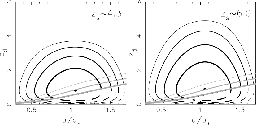
Figure 1: Contours of joint probability of multiple image optical depth for $\sigma/\sigma_{\star}$ and $z_{\rm d}$ assuming lens galaxies fainter than $i^{*}_{gal}=22.2$ (solid contours), and for all lens galaxies (dashed contours). The dots are placed at the distribution mode, and the contours are plotted at 1/3, 1/9, 1/27 and 1/81 the peak height. The thick grey line shows the locus of galaxies having $i^{*}_{gal}=22.2$, the thinner grey line $i^{*}_{gal}=23.2$ and the thinnest grey line $i^{*}_{gal}=24.2$.

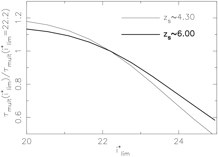
Figure 2: The multiple image optical depth $\tau_{mult}$ for different bright lens galaxy limits $i^{*}_{gal}$, normalized by the optical depth for a limit of $i^{*}_{gal}=22.2$.

Figure 1 shows the joint probability contours of multiple image optical depth for $\sigma/\sigma_{\star}$ and $z_{\rm d}$ assuming sources at redshifts of $z_{\rm s}\sim 4.3$ (left) and $z_{\rm s}\sim 6.0$ (right). The solid contours represent the undetected lens galaxies which are included in calculations of the lensing statistics through the remainder of this paper, and the dashed lines represent the rest of the potential lens galaxy population. The $i^{*}_{gal}=22.2$ borderline that separates these populations of galaxies is also shown. The fraction of the lens population lost due to the requirement of non-detectability of the lens galaxy is 20–30%. Figure 1 also shows loci corresponding to $i^{*}_{gal}=23.2$ and 24.2. These give an indication of the effect on lens statistics of disregarding still fainter lens galaxies. As a further guide to the sensitivity of the lens statistics on the assumed bright lens galaxy limit, we have computed the optical depth for different bright lens galaxy limits and plotted them as a fraction of the optical depth for a limit of $i^{*}_{gal}=22.2$ in Figure 2. This figure may be used to estimate the variation of the lensing probabilities calculated in this paper with the absence of lens galaxies brighter than different limiting values $i^{*}_{gal}$. For example, excluding lens galaxies down to $i^{*}_{gal}=23.2$ will reduce the multiple imaging rates presented in this paper to $\sim 80-90\%$ of their quoted values. In addition to the aforementioned samples we will also consider for reference the statistics of lensing by the entire E/S0 galaxy population of quasars with $z_{\rm s}=2.1$.

The galaxy mass distribution is modeled as a combination of stars and a smooth dark matter halo having in total a mass profile of a singular isothermal sphere (SIS). The stars are distributed according to de-Vaucouleurs profiles having characteristic radii and surface brightnesses determined as a function of $\sigma_{star}$ from the relations of Djorgovski & Davis (1987). A constant mass-to-light ratio as a function of radius is assumed. The inclusion of stars allows us to calculate three possible effects due to microlensing: (i) a possible increase in the magnification of bright quasars; (ii) short-term variability of the quasar flux; and (iii) changes in the equivalent width of the broad emission lines in the quasar spectrum due to differential magnification of the continuum and emission-line regions. We compute the microlensing statistics by convolving a large number of numerical magnification maps with the distribution of microlensing optical depth and shear for lines of sight to random source positions (Wyithe & Turner 2002). We assume a source size of $10^{15}{\rm cm}$ (corresponding to 10 Schwarzschild radii of a $3\times 10^{8}M_{\odot}$ black hole) and microlens masses of $0.1M_{\odot}$. The microlens surface mass density is evolved with redshift in proportion to the fraction of the stellar mass that had formed by that redshift. We assume a constant star formation rate at $z>1$ and a rate proportional to $(1+z)^{3}$ at $z<1$ (Hogg 1999 and references therein; Nagamine, Cen & Ostriker 2000). The mass-to-light ratios were normalized so that the elliptical/S0 plus spiral populations at redshift zero contain a cosmological density parameter in stars of $\Omega_{\star}=0.005$ (Fukugita, Hogan & Peebles 1998). The model for elliptical galaxies therefore has two characteristic angular scales. On arcsecond scales the mass distribution follows the radial profile of an isothermal sphere (which determines the macrolensing cross-section). On micro-arcsecond scales, the grainy mass distribution of the stars yields different phenomena related to microlensing.

The inclusion of non-sphericity in the lenses is beyond the scope of this paper. Although previous studies (Kochanek & Blandford 1987; Blandford & Kochanek 1987) found that the introduction of ellipticities $\lesssim 0.2$ into nearly singular profiles has little effect on the lensing cross-section and image magnification, the strong magnification bias will favor a high fraction of 4-image lenses (Rusin & Tegmark 2001) as well as an increase in the number of multiple image systems. One consequence of this effect will be to double the expected microlensing rate (see §6). We also do not include source extinction by the lens galaxy, which should arise primarily in the rarer spiral galaxy lenses. Spiral galaxies may be more common at the higher lens redshifts encountered for the high redshift quasar catalogs, and should be considered in future extensions of this work.

2.2 Magnification Distribution

We define $dP/d\mu$ as the normalized differential probability per unit magnification and $\tau_{mult}$ as the multiple-image optical depth. The magnification distributions were computed for singly-imaged quasars [$(1-\tau_{mult})\frac{dP_{sing}}{d\mu}$], multiply-imaged quasars [$\tau_{mult}\frac{dP_{mult}}{d\mu}$, where $\mu$ is the sum of the multiple image magnifications], and all quasars [$\frac{dP_{tot}}{d\mu}=(1-\tau_{mult})\frac{dP_{sing}}{d\mu}+\tau_{mult}\frac{dP_{mult}}{d\mu}$]. These are illustrated in Figure 3 for $z_{\rm s}=2.1$ (top column), $z_{\rm s}=4.3$ (central column) and $z_{\rm s}=6.0$ (lower column). The histograms show the spread resulting from microlensing around the usual SIS distributions (which are shown for comparison by the dot-dashed lines), including a non-zero probability for single images with magnifications larger than 2, and a nonzero probability for the total magnification of a multiply-imaged source to be smaller than 2. The method described in Wyithe & Turner (2002) does not determine the magnification along all lines of sight. Specifically, those source positions whose lines of sight have microlensing optical depth $\kappa<10^{-4}$ and hence magnifications near 1 are not considered. However the average magnification for a random source position must be unity, and we add probability smoothly to the single image distribution in the bins between 0.9 and 1.1 such that [$\frac{dP_{tot}}{d\mu}$] has unit mean and [$(1-\tau_{mult})\frac{dP_{sing}}{d\mu}$] is normalized to $1-\tau_{mult}$. The detail of the treatment of the distributions near $\mu=1$ has no barring on the resulting lens statistics.

In order to find the fraction of multiply-imaged sources, the magnification distributions need to be convolved with the quasar luminosity function. We discuss the luminosity function next.

2.3 Quasar Luminosity Function

The standard double power-law luminosity function (Boyle, Shanks & Peterson 1988; Pei 1995) for the number of quasars per comoving volume per unit luminosity

$$\phi(L,z_{\rm s})=\frac{\phi_{\star}/L_{\star}(z_{\rm s})}{[L/L_{\star}(z_{\rm s})]^{\beta_{l}}+[L/L_{\star}(z_{\rm s})]^{\beta_{h}}}$$ (2)

provides a successful representation of the observed quasar luminosity function at redshifts $\lesssim 3$. The functional dependence on redshift is in the break luminosity $L_{\star}$ indicating pure luminosity evolution. At $z_{\rm s}\ll 3$ the break luminosity evolves as a power-law in redshift and the number counts increase with redshift; higher redshift surveys indicate that there is a decline in the space density of bright quasars beyond $z_{\rm s}\sim 3$ (Warren, Hewett & Osmer 1994; Schmidt, Schneider & Gunn 1995; Kennefick, Djorgovski & de Carvalho 1995). Madau, Haardt & Rees (1999) suggested an analytic form for the evolution of $L_{\star}$ of the form

$$L_{\star}(z_{\rm s})=L_{\star,0}(1+z_{\rm s})^{-(1+\alpha)}\frac{e^{\zeta z_{\rm s}}(1+e^{\xi z_{\star}})}{e^{\xi z_{\rm s}}+e^{\xi z_{\star}}},$$ (3)

where $\alpha$ is the slope of the power-law continuum of quasars (taken to be -0.5 throughout this paper). Fan et al. (2001b) found from their sample of SDSS quasars at $z_{\rm s}\sim 4.3$ that the slope of the bright end of the luminosity function has evolved to $\beta_{h}\sim 2.58$ from the $z_{\rm s}\sim 3$ value of $\beta_{h}\sim 3.43$. This result supported the findings of Schmidt, Schneider & Gunn (1995). We therefore consider two luminosity functions in this study. In one case we consider $\beta_{h}=3.43$ below $z_{\rm s}=3$ and $\beta_{h}\sim 2.58$ above $z_{\rm s}=3$. As a second case, we assume that the slope of the bright end $\beta_{h}=3.43$ does not evolve above $z_{\rm s}\sim 3$ and so we adopt pure luminosity evolution at all redshifts. We emphasize that while $\beta_{h}=3.43$ is found not to vary at $z_{\rm s}\lesssim 3$, the (small) samples of quasars at $z_{\rm s}\gtrsim 4$ suggest the flatter slope ($\beta_{h}=2.58$) for the bright end of the luminosity function. Thus currently a luminosity function having $\beta_{h}=2.58$ best fits the high redshift data. In the remainder of the paper, discussions of numerical results will list those for $\beta_{h}=2.58$ first.

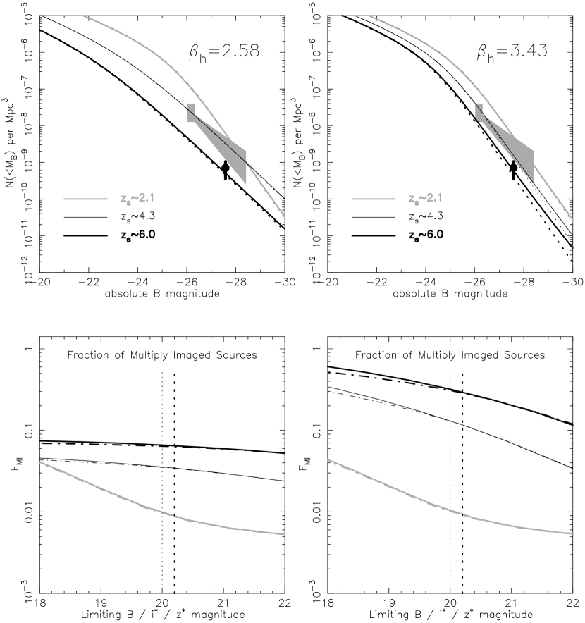
Figure 4: Upper panels: The cumulative quasar luminosity functions at $z_{\rm s}\sim 2.1$ (thick light lines), $z_{\rm s}\sim 4.3$ (thin dark lines) and $z_{\rm s}\sim 6.0$ (thick dark lines). The solid and dotted lines show the lensed and intrinsic luminosity functions, respectively. The solid grey region represents the non-parametric luminosity function from the SDSS $z_{\rm s}\sim 4.3$ quasar sample (Fan et al. 2001b), and the dark point with vertical error bar shows the measured space density of quasars at $z_{\rm s}\sim 6.0$ (Fan et al. 2001c). The left and right panels show luminosity functions with $\beta_{h}=3.43$ for $z_{\rm s}<3$ but $\beta_{h}=2.58$ and $\beta_{h}=3.43$ respectively for $z_{\rm s}>3$. Lower panels: The fraction, $F_{\rm MI}$, of multiply-imaged quasars with redshifts $z_{\rm s}\sim 2.1$, $4.3$ and $6.0$, as a function of limiting $B$, $i^{*}$ and $z^{*}$ magnitudes, respectively. The solid and dot-dashed lines correspond to calculations that include microlensing and those that only consider a smooth lensing mass distribution. The limiting magnitudes are marked by the vertical dotted lines, and the line types are the same as in the upper panels.

With the above two prescriptions, the evolution of $L_{\star}$ is adjusted to adequately describe the low redshift luminosity function (Hartwick & Schade 1990), and the space density of quasars at $z_{\rm s}\sim 4.3$ and $z_{\rm s}\sim 6$ measured by Fan et al. (2001b,c). The resulting luminosity functions at $z_{\rm s}\sim 2.1$, $z_{\rm s}\sim 4.3$ and $z_{\rm s}\sim 6.0$ are plotted in the upper panels of Figure 4 and the corresponding parameters for equations (2) and (3) are listed in Table 3. The dotted line shows the unlensed luminosity function and the solid line shows the lensed luminosity function (e.g. Pei 1995b) including microlensing. Note that for $\beta_{h}=3.43$ the number density of quasars at $z_{\rm s}\sim 6.0$ with $M_{B}<-27.6$ is increased by a factor of $\sim 1.5$ due to lensing. For the computation of lens statistics for flux limited samples of quasars we use the cumulative version of equation (2), namely $N(>L,z_{\rm s})=\int_{L}^{\infty}dL^{\prime}\phi(L^{\prime},z_{\rm s})$.

3 Multiple Imaging Rates

We now combine the magnification distributions described in §2.2 with the luminosity functions of §2.3 to find the fraction of multiply imaged quasars,

$$F_{\rm MI}(z_{\rm s})=\frac{\int_{0}^{\infty}d\mu^{\prime}\tau_{\rm mult}\frac{dP_{\rm mult}}{d\mu^{\prime}}N(>\frac{L_{\rm lim}}{\mu^{\prime}},z_{\rm s})}{\int_{0}^{\infty}d\mu^{\prime}\left[\tau_{\rm mult}\frac{dP_{\rm mult}}{d\mu^{\prime}}+(1-\tau_{\rm mult})\frac{dP_{\rm sing}}{d\mu^{\prime}}\right]N(>\frac{L_{\rm lim}}{\mu^{\prime}},z_{\rm s})},$$ (4)

where the multiple image optical-depth obtains values of $\tau_{\rm mult}=0.0019$, 0.0040 and 0.0059 for $z_{\rm s}=2.1$, 4.3 and 6.0 respectively, and $L_{lim}$ is the limiting luminosity at a redshift $z_{\rm s}$ corresponding to the limiting survey magnitude $m_{lim}$. The limiting luminosity $L_{\rm lim}$ was determined from $m_{lim}$ using the luminosity distance for the assumed cosmology and a $k$-correction computed from a model quasar spectrum including the mean absorption by the intergalactic medium (M$\o$ller & Jakobsen 1990; Fan 1999). Note that equation (4) reduces to the usual approximation for magnification bias in the limit of small $\tau_{mult}$ and shallow luminosity functions.

The lower panels of Figure 4 show the predicted lens fraction for samples of quasars at $z_{\rm s}\sim 2.1$ (thick light lines), $z_{\rm s}\sim 4.3$ (thin dark lines) and $z_{\rm s}\sim 6.0$ (thick dark lines) as a function of the limiting survey magnitude. The solid lines show the fraction found when microlensing is included while the dot-dashed lines show results for pure SIS lenses. Results have been computed for the two luminosity functions discussed in §2.3. The vertical lines mark the limiting magnitudes for the high redshift samples, namely $i^{*}\sim 20.0$ for the $z_{\rm s}\sim 4.3$ survey and $z^{*}\sim 20.2$ for the $z_{\rm s}\gtrsim 5.8$ survey. The magnification bias and hence the multiple image fraction is significantly higher for brighter limiting magnitudes. The lens fraction asymptotes to a constant value at the brighter limits considered here since these are sufficiently brighter than the break magnitude that only very large and hence rare magnifications could result in the inclusion of quasars fainter than $L_{\star}$. Therefore at these bright limits the luminosity function can be considered as a single power-law with a resulting bias that is insensitive to the limiting magnitude. Obviously a steeper bright end slope leads to a larger magnification bias and a higher multiple image fraction. We find that a typical survey of quasars at low redshift ($z_{\rm s}\sim 2.1$) has $F_{\rm MI}\sim 0.01$ (for a limiting B-magnitude of $m_{B}=20$). This estimate is consistent with the measured lens fraction in the HST Snapshot Survey (Maoz et al. 1993). However as argued by Barkana & Loeb (2000), bright high redshift quasar surveys should find much higher values of $F_{\rm MI}$. For $\beta_{h}=2.58$ we find $F_{\rm MI}\sim 0.04$ at $z_{\rm s}\sim 4.3$ and $F_{\rm MI}\sim 0.07$ at $z_{\rm s}\sim 6.0$, respectively. For $\beta_{h}=3.43$ the fractions are even higher, $F_{\rm MI}\sim 0.13$ at $z_{\rm s}\sim 4.3$ and $F_{\rm MI}\sim 0.30$ at $z_{\rm s}\sim 6.0$ respectively. Note the inferred absolute quasar luminosity is quite sensitive to the $k$-correction, particularly from the absorption spectrum since quasars at $z_{\rm s}\sim 6$ are nearly completely absorbed blueward of Ly$\alpha$. As a result the inferred lens fraction for a fixed apparent magnitude limit is also sensitive to the $k$-correction. However we find that microlensing makes little difference to the multiple imaging fraction unless the survey limit is very bright.

We have extrapolated the luminosity function at $z_{\rm s}\sim 4.3$ and $z_{\rm s}\sim 6$ from the well-studied luminosity function at lower redshifts. We now consider how the results may be affected should this extrapolation be invalid. Conversely, given the large multiple image fraction it may be possible in the future to use the observed fraction of multiple images in these samples to constrain properties of the luminosity function (modulo systematics in lens modeling and cosmology). As a demonstration of this potential use, we calculate multiple image fractions for sources at $z_{\rm s}\sim 4.3$ with $i^{*}<20.0$ and at $z_{\rm s}\sim 6.0$ with $z^{*}<20.2$ assuming values of break luminosity that are within factors of 10 above and below the corresponding values of $L_{\star}$ listed in Table 3. The results are plotted in Figure 5 (line types as in Figure 4). We see that the multiple image fraction is rather insensitive to the location of the break for the shallow ($\beta_{h}=2.58$) luminosity function. However the location of the break plays a more significant role for the steep ($\beta_{h}=3.43$) luminosity function, particularly at $z_{\rm s}\sim 4.3$ where the limiting magnitude is closer to the extrapolated location of the break.

4 Magnification of Observed Sources

In §2.2 we considered the probability of magnification along lines of sight to random sources. In this section we expand on the discussion in Wyithe & Loeb (2002) and calculate the a-posteriori probability for the magnification of a known quasar in the high-redshift samples. If a quasar is observed with a magnification of $\mu_{obs}$, then it is intrinsically fainter by a factor of $\mu_{obs}$ and therefore more abundant by a factor of $[\phi(L/\mu_{obs})/(\mu_{obs}\phi(L))]$. The distribution of magnifications observed at redshift $z_{\rm s}$ in a flux-limited sample is

$$\frac{dP}{d\mu_{\rm obs}}=\frac{\left[\tau_{\rm mult}\frac{dP_{\rm mult}}{d\mu}|_{\mu=\mu_{\rm obs}}+(1-\tau_{\rm mult})\frac{dP_{\rm sing}}{d\mu}|_{\mu=\mu_{\rm obs}}\right]N(>\frac{L_{\rm lim}}{\mu_{\rm obs}})}{\int_{0}^{\infty}d\mu^{\prime}\left[\tau_{\rm mult}\frac{dP_{\rm mult}}{d\mu}|_{\mu=\mu^{\prime}}+(1-\tau_{\rm mult})\frac{dP_{\rm sing}}{d\mu}|_{\mu=\mu^{\prime}}\right]N(>\frac{L_{\rm lim}}{\mu^{\prime}})}.$$ (5)

The bias in this equation introduces additional skewness into the magnification distribution. This effect is particularly severe for the high-redshift samples in which quasars are selected to be bright (so that they reside in the steep part of the luminosity function).

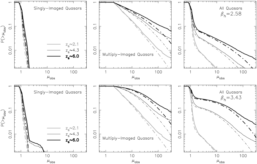
Figure 6: The probability for observing a magnification larger than $\mu_{\rm obs}$ of quasars in flux-limited samples. The left, center and right panels show distributions for singly-imaged quasars, for the sum of images of a multiply-imaged quasar, and for the combination of the two (i.e. all quasars). The upper and lower panels show results for luminosity functions with $\beta_{h}=3.43$ for $z_{\rm s}<3$ but $\beta_{h}=2.58$ and $\beta_{h}=3.43$ respectively for $z_{\rm s}>3$. In each panel we show the distributions at quasar redshifts of $z_{\rm s}\sim 2.1$ (thick light lines), $z_{\rm s}\sim 4.3$ (thin dark lines) and $z_{\rm s}\sim 6.0$ (thick dark lines) for limiting magnitudes of $m_{B}=20.0$, $i^{*}=20.0$ and $z^{*}=20.2$ respectively. The solid and dot-dashed lines correspond to calculations that include microlensing and those that only consider a smooth lensing mass distribution, respectively.

Figure 6 shows the cumulative distributions of observed magnifications for sources at redshifts $z_{\rm s}\sim 2.1$, $4.3$ and $6.0$ (line types as in Figure 4) in samples of quasars with $m_{B}<20.0$, $i^{*}<20.0$ and $z^{*}<20.2$ respectively. Distributions are shown for single images, for the sum of multiple images and for all images. The upper and lower panels show results for luminosity functions with $\beta_{h}=2.58$ and $\beta_{h}=3.43$ (at $z_{\rm s}>3$), respectively. The distributions are highly skewed, having medians near unity but means as high as a few tens (values are listed in Table 3). Note that with $\beta_{h}=3.43$, multiple images generate a fairly flat distribution out to high magnifications for the $z_{\rm s}\sim 4.3$ and $z_{\rm s}\sim 6.0$ samples. This follows from the fact that at luminosities above $L_{\star}$ the integrated luminosity function is nearly as steep as the high magnification tail of the magnification distribution. As a result of microlensing the single image distributions show a small probability for magnifications larger than 2. Microlensing also causes a significant increase in the probability of observing the very largest magnifications in multiply-imaged sources. Highly magnified multiple images are more likely in the high redshift samples because of the larger magnification bias. This trend combined with the fact that multiple images are more common in general at high redshift results in a very large difference between the probabilities of observing $\mu_{\rm obs}>10$ at the different redshifts considered.

The a-posteriori multiple image fraction and distribution of magnifications observed for sources having a luminosity $L$ and a redshift $z_{\rm s}$ are

$$F_{\rm MI}(z_{\rm s})=\frac{\int_{0}^{\infty}d\mu^{\prime}\tau_{\rm mult}\frac{dP_{\rm mult}}{d\mu^{\prime}}\frac{\phi(L/\mu^{\prime},z_{\rm s})}{\mu^{\prime}}}{\int_{0}^{\infty}d\mu^{\prime}\left[\tau_{\rm mult}\frac{dP_{\rm mult}}{d\mu^{\prime}}+(1-\tau_{\rm mult})\frac{dP_{\rm sing}}{d\mu^{\prime}}\right]\frac{\phi(L/\mu^{\prime},z_{\rm s})}{\mu^{\prime}}},$$ (6)

and

$$\frac{dP}{d\mu_{\rm obs}}=\frac{\left[\tau_{\rm mult}\frac{dP_{\rm mult}}{d\mu}|_{\mu=\mu_{\rm obs}}+(1-\tau_{\rm mult})\frac{dP_{\rm sing}}{d\mu}|_{\mu=\mu_{\rm obs}}\right]\frac{\phi(L/\mu_{\rm obs})}{\mu_{obs}}}{\int_{0}^{\infty}d\mu^{\prime}\left[\tau_{\rm mult}\frac{dP_{\rm mult}}{d\mu}|_{\mu=\mu^{\prime}}+(1-\tau_{\rm mult})\frac{dP_{\rm sing}}{d\mu}|_{\mu=\mu^{\prime}}\right]\frac{\phi(L/\mu^{\prime})}{\mu^{\prime}}}.$$ (7)

We have calculated these quantities for the 4 SDSS $z_{\rm s}\gtrsim 5.8$ quasars discovered by Fan et al. (2000; 2001c). The results are plotted in Figure 7, and the resulting medians, means and multiple imaging fractions are listed in Table 3. Assuming $\beta_{h}=2.58$ (3.43) the probability for multiple imaging is $F_{\rm MI}\sim 0.06-0.07$ ($0.3-0.4$) for these quasars, with expected magnifications of $\langle\mu_{\rm obs}\rangle\sim 4.5-5.5$ ($23-50$). Thus, if the bright end of the luminosity function is shallow ($\beta_{h}=2.58$) as suggested by Fan et al. (2001b) then we do not expect any lenses among the existing $z_{\rm s}\gtrsim 5.8$ sample. On the other hand, if $\beta_{h}=3.43$ (as extrapolated from the pure luminosity evolution observed at low redshifts) then we expect one or two out of the four $z_{\rm s}\gtrsim 5.8$ quasars to be multiply imaged and magnified by a large factor, while the others should have magnifications $\lesssim 2$.

5 Lens Galaxy Light and the Gunn-Peterson Trough

The spectra of quasars at $z_{\rm s}\sim 6$ provide an exciting probe of the epoch of reionization. The spectrum of the very highest redshift quasar discovered to date was found by Becker et al. (2001) to have higher than expected neutral hydrogen absorption, indicating a possible Gunn-Peterson trough due to the pre-ionized intergalactic medium (Gunn & Peterson 1965). While we have required that lens galaxies not be detected by the SDSS imaging survey, it is possible that lens galaxies would contribute flux in deeper follow-up observations. The high fraction of lensed quasars expected in the SDSS catalog at $z_{\rm s}\sim 6$ implies that light from the lens galaxy may contaminate the Gunn-Peterson trough for a substantial fraction of all quasars. This has the potential to limit the ability of deep spectroscopic observations to probe the evolution of the neutral hydrogen fraction during the epoch of reionization in some cases.

We have estimated the distribution of flux per unit wavelength, $f_{\lambda}$, in the Gunn-Peterson trough due to lens galaxy light for multiply-imaged $z_{\rm s}\sim 6$ quasars as a function of lens galaxy velocity dispersion and redshift, and convolved the result with the joint probability distribution shown in Figure 1. We used the $i^{*}$-band absolute magnitude of an $L_{\star}$ early-type galaxy (Madgwick et al. 2001; and color corrections from Fukugita, Shimasaku & Ichikawa 1995 and Blanton et al. 2001) and computed the apparent flux assuming the Faber-Jackson (1976) relation, the mean galaxy spectrum from Kennicutt (1992), and a rest-frame mass-to-light ratio that evolves as $\frac{dlog(M/L)}{dz}=-0.6$ (Koopmans & Treu 2001). We further assumed that all of the galaxy light is added to the quasar spectrum. Figure 8 shows the probability that flux at a level greater than $f_{\lambda}$ will be observed in the Gunn-Peterson trough. Probabilities are shown assuming lens galaxies fainter than $i^{*}_{gal}=22.2$, 23.2 and 24.2. The spectra of the $z_{\rm s}=6.28$ quasar published by Becker et al. (2001) and Pentericci (2001) show that the flux in the Gunn-Peterson trough is $\lesssim 3\times 10^{-19}{\rm\,erg\,sec\,cm^{-2}\,\AA}$. We estimate that $\sim 40\%$ of lens galaxies should contribute flux above this level ($i^{*}_{gal}=22.2$). Hence, the observed flux limit in the Gunn-Peterson trough does not rule out lensing for this object. On the other hand the probability is not negligible and demonstrates the need to account for the possibility of a contaminating lens galaxy.

6 Microlensing and the High-redshift Quasar Samples

So far, we have found that the rare high magnifications caused by microlensing due to stars do not significantly affect the multiple image fraction, but do result in a significant excess of the highest magnifications. We now consider more direct manifestations of microlensing. In particular, we compute the fraction of all quasars that should vary by more than $\Delta m$ magnitudes during a 10 year period, and the expected microlensing-induced distortion of the distribution of equivalent widths for the broad emission lines of quasars. The results in this section have been computed assuming a luminosity function having $\beta_{h}=3.43$ at all redshifts, which yield larger lensing fractions as discussed in previous sections. However we point out how the results can be applied to the case of $\beta_{h}=2.58$ where appropriate.

6.1 Quasar Flux Variability due to Microlensing

Microlensing induces quasar variability due to the relative angular motion of the observer, lens and source. The variability occurs on a shorter timescale for lens galaxies at lower redshifts due to the larger projected transverse velocity. Since the SDSS high-redshift samples select against low-redshift lens galaxies, we expect measurable microlensing variability to be rare. On the other hand, the high magnification bias for these samples suggests a high multiple imaging rate and a large galaxy-quasar angular correlation, bringing more lines of sight to regions on the sky with a significant microlensing optical depth. We have computed the fraction of quasar images that vary by more than $\Delta m$ magnitudes during the 10 years following discovery using the methods described in Wyithe & Turner (2002). Magnification bias is calculated based on the magnification of the first light-curve point (the sum of magnifications for a multiply-imaged source). The effective transverse source plane velocity was computed from the two transverse velocity components for each of the source, lens and observer (Kayser, Refsdal & Stabell 1986). We assume each component to be Gaussian-distributed with a dispersion of 400${\rm\,km\,sec^{-1}}$.

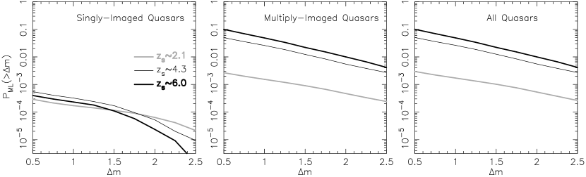
Figure 9: The fraction of quasars that are microlensed by more than $\Delta m$ during the 10 years following their discovery. The left, center and right panels show results for singly-imaged quasars, for the images of a multiply-imaged quasar (with each image considered separately), and for all quasars. The luminosity function is assumed to have $\beta_{h}=3.43$ at all redshifts. In each panel we show results at quasar redshifts of $z_{\rm s}\sim 2.1$ (thick light lines), $z_{\rm s}\sim 4.3$ (thin dark lines) and $z_{\rm s}\sim 6.0$ (thick dark lines) for limiting magnitudes of $m_{B}=20.0$, $i^{*}=20.0$ and $z^{*}=20.2$ respectively.

Figure 9 shows the resulting probabilities for the variability amplitude of quasars at $z_{\rm s}\sim 2.1$, $4.3$ and $6.0$, with line types as in Figure 4. The fraction of quasars that are singly-imaged and microlensed is shown in the left panel, the fraction of quasar images (counting each image separately) that appear in multiple image systems and are microlensed is shown in the central panel, and the fraction of all quasar images to be microlensed is shown in the right panel. Microlensing variability is dominated by multiple-image systems. This is particularly true for the high redshift samples, where the high magnification bias results in a large multiple-image fraction. While only 1 in 300 images at $z_{\rm s}\sim 2.1$ vary by more than $\Delta m=0.5$ magnitudes, we find that at $z_{\rm s}\sim 6$ the fraction has risen to $\sim 10\%$. The fraction of quasars at $z_{\rm s}\sim 6$ that are multiply-imaged and microlensed assuming the flat luminosity function having $\beta_{h}=2.58$ is approximately obtained by multiplying the above result by $0.07/0.30$ to correct for the multiple image rate.

Since the multiple image fraction is $\sim 0.3$ we find that $\sim 1$ in 3 multiply-imaged quasars at $z_{\rm s}\sim 6$ will show microlensing of more than $\Delta m=0.5$ magnitudes in one of their images during the 10 years following discovery. Similarly we find that at $z_{\rm s}\sim 4.3$, $\sim 5\%$ of quasars will vary by more than $\Delta m=0.5$ magnitudes. Since the multiple image fraction is $\sim 0.13$, this indicates that $\sim 1$ in 3 multiply-imaged sources will exhibit microlensing above this level in one of their images. These fractions hold if $\beta_{h}=2.58$. Quasars also vary intrinsically. However, while microlensing causes independent variability of the quasar images, intrinsic variability is observed in all images separated by the lens time delay (e.g. Kundic et al. 1997). After the lens time delay is determined, it should be possible to separate microlensing variability from intrinsic variability.

The SDSS is expected to discover $\sim 30$ quasars with $z_{\rm s}\gtrsim 5.8$ when completed. If $\beta_{h}=3.43$, monitoring of these quasars should yield $\sim 3$ microlensing events. Unlike lensed quasars with lens galaxies having $z_{\rm d}\ll 1$, the source to lens angular diameter distance ratio in these cases is near unity. The source size is therefore comparable to the projected microlens Einstein radius and so proposed caustic crossing experiments to map the structure of the accretion disc (e.g. Agol & Krolik 1999) will not be applicable. Nonetheless, the microlens Einstein radius still represents an interesting characteristic scale, and the detection of microlensing would provide an upper limit on the extent of the source size. If the source emission is interpreted as originating from a smooth accretion disk, then microlensing variability would place an upper limit on the mass of the quasar black hole. This, in turn, would yield a lower limit on the ratio between the quasar luminosity and its maximum (Eddington) value which would be useful in constraining models for early structure formation (Haiman & Loeb 2001).

6.2 Distortion in the Equivalent Width Distribution of Quasar Emission Lines

Fan et al. (2001c) noted that their high redshift quasar ($z>5.8$) selection criteria favor objects with strong emission lines (particularly Ly$\alpha$). Since microlensing results in variability of emission-line equivalent-widths by differentially magnifying the compact continuum region compared to the more extended region that produces the lines (Canizares 1982; Delcanton et al. 1994; Perna & Loeb 1998), it is important to quantify how large this effect might be in the high-redshift quasar samples. We follow Perna & Loeb (1998) and compute the distribution of relative magnifications ${dP}/{d(\mu/\langle\mu\rangle)}$ (where $\langle\mu\rangle$ is the mean magnification near the line of sight) which is then convolved with the intrinsic log-normal equivalent width distribution. We consider magnification bias when constructing ${dP}/{d(\mu/\langle\mu\rangle)}$. Microlensing is more likely to lower the observed equivalent width because sources are more likely to be selected when their continuum magnification is above the average. Results are shown in Figure 10 for the $z_{\rm s}\sim 2.1$ (upper row), $z_{\rm s}\sim 4.3$ (central row), and $z_{\rm s}\sim 6.0$ (lower row) samples. The distributions for singly imaged sources show almost no departure from the intrinsic distribution, while the median of the multiply-imaged source distribution is lowered by $\sim 10\%$, $\sim 20\%$ and $\sim 30\%$ respectively for the $z_{\rm s}\sim 2.1$, $4.3$, and $6.0$ samples. These values are slightly reduced if $\beta_{h}=2.58$. Microlensing results in a net reduction in the median equivalent width for $z_{\rm s}\sim 6.0$ quasars of $\sim 15\%$ relative to its intrinsic value. Thus, we expect the observed equivalent width distribution to be altered from its intrinsic state, but the level of variation to be smaller than the intrinsic spread. Hence, the distortion of equivalent widths due to microlensing should not bias against the selection of lensed quasars in the sample of Fan et al. (2000c).

7 Summary

We have shown that gravitational lensing should be more common by 1–2 orders of magnitude in the high-redshift quasar catalogs at $z_{\rm s}\sim 4.3$ and $z_{\rm s}\gtrsim 5.8$ recently published by the Sloan Digital Sky Survey (SDSS), as compared to previous quasar samples. The reasons for this large increase are twofold. First, the optical depth for multiple imaging increases with redshift. Second, all quasars in the SDSS high redshift catalogs populate the bright end of the luminosity function making the magnification bias stronger. Using extrapolations of the luminosity function having bright-end slopes of $-2.58$ (suggested by observations at $z_{\rm s}\sim 4.3$) and $-3.43$ (found at all $z_{\rm s}\lesssim 3$) we find that multiple image fractions of $\sim 4\%$ $(13\%)$ for quasars at $z_{\rm s}\sim 4.3$ (brighter than $i^{*}=20.0$) and $\sim 7\%$ ($30\%$) for quasars at $z_{\rm s}\sim 6.0$ (brighter than $z^{*}=20.2$). These fractions depend sensitively on the value of the break luminosity and the bright-end slope. Thus, the observed lensing rate in these bright samples can be used to constrain the parameters of the quasar luminosity function at high redshifts.

We have computed the distribution of magnifications for quasars in flux limited samples. A steep bright-end slope results in high probabilities for very large magnifications because the slope of the luminosity function is comparable to the slope of the high magnification tail of the magnification distribution. Assuming bright end luminosity function slopes of $-2.58$ and $-3.43$, the median and mean magnifications are $med(\mu_{obs})=1.02$ (1.09) and $\langle\mu_{obs}\rangle=2.09$ (6.00) for quasars at $z_{\rm s}\sim 4.3$ (brighter than $i^{*}=20.0$), and $med(\mu_{obs})=1.09$ (1.19) and $\langle\mu_{obs}\rangle=4.55$ (23.0) for quasars at $z_{\rm s}\sim 6.0$ (brighter than $z^{*}=20.2$). The considerable abundance of systems with high magnifications implies that estimates of the quasar luminosity density need to be done with care after taking out gravitationally lensed systems.

Observations of the highest redshift quasar ($z_{\rm s}=6.28$) show a complete Gunn-Peterson trough at a level $<3\times 10^{-19}{\rm\,erg\,sec\,cm^{-2}\,\AA}$. We find that $\sim 40\%$ of multiple image lens galaxies (fainter than $i^{*}_{gal}=22.2$) will contribute flux in the Gunn-Peterson trough (of a $z_{\rm s}\sim 6$ quasar) at a level above $3\times 10^{-19}{\rm\,erg\,sec\,cm^{-2}\,\AA}$. For some quasars the contamination of the Gunn-Peterson trough with flux from lens galaxies may therefore limit the ability of deep spectroscopic observations to probe the evolution of the neutral hydrogen fraction during the epoch of reionization.

We have also computed microlensing statistics for high redshift quasars in flux limited samples, and found that microlensing will be dominated by multiply-imaged sources. One third of multiply-imaged quasars at $z_{\rm s}\sim 4.3$ (brighter than $i^{*}=20.0$) and one third of multiply-imaged quasars at $z_{\rm s}\sim 6.0$ (brighter than $z^{*}=20.2$) will vary due to microlensing by more than 0.5 magnitudes during the decade following discovery. This variability allows for the exciting possibility of using differential microlensing magnification to probe the smallest scales of bright quasars beyond a redshift of 6. Finally, we find that microlensing lowers the median of the distribution of emission-line equivalent-widths for multiply-imaged quasars at $z_{\rm s}\sim 6.0$ (brighter than $z^{*}=20.2$) by $\sim 15\%$ relative to its intrinsic value. This effect is smaller than the intrinsic spread and should therefore not bear on the quasar selection function.

Figure 3: Magnification distributions for quasars. The left, center and right panels show distributions for singly-imaged quasars, for the sum of images of multiply-imaged quasars, and for the combination of the two (i.e. all quasars). The top, central and lower rows show cases where $z_{\rm s}\sim 2.1$, $z_{\rm s}\sim 4.3$ and $z_{\rm s}\sim 6.0$.

Figure 5: The fraction, $F_{\rm MI}$, of multiply-imaged quasars $z_{\rm s}\sim 4.3$ (thin dark lines) and $z_{\rm s}\sim 6.0$ (thick dark lines) for limiting magnitudes of $i^{*}=20.0$ and $z^{*}=20.2$ respectively, as a function of the break luminosity in units of the value quoted in Table 3. The left and right panels show luminosity functions with $\beta_{h}=3.43$ for $z_{\rm s}<3$ but $\beta_{h}=2.58$ and $\beta_{h}=3.43$ respectively for $z_{\rm s}>3$. The solid and dot-dashed lines correspond to calculations that include microlensing and those that only consider a smooth lensing mass distribution, respectively.

Figure 7: The probability of observing a magnification larger than $\mu_{\rm obs}$ for quasars having the fluxes and redshifts of the four SDSS $z_{\rm s}\gtrsim 5.8$ quasars. The thin and thick lines show results for luminosity functions with $\beta_{h}=3.43$ for $z_{\rm s}<3$ but $\beta_{h}=2.58$ and $\beta_{h}=3.43$ respectively for $z_{\rm s}>3$. The solid and dot-dashed lines correspond to calculations that include microlensing and those that only consider a smooth lensing mass distribution, respectively. In Table 3 we list the multiple image probability, $F_{\rm MI}$, and the distribution mean, $\langle\mu_{obs}\rangle$, and median, $med(\mu_{obs})$, for each of these quasars.

Figure 8: The probability that a lens galaxy responsible for a multiply imaged quasar will contribute a flux greater than $f_{\lambda}$ in the Gunn-Peterson trough of a quasar at $z_{\rm s}\sim 6$. Three lines are shown corresponding to lens galaxies fainter than $i^{*}_{gal}=22.2$, 23.2 and 24.2 (thicker lines denote brighter magnitude limits).

Figure 10: The microlensed distribution (solid lines) of equivalent-widths ($W$) for the broad emission lines of quasars. The left, center and right panels show results for singly-imaged quasars, for the sum of images in multiply-imaged quasars, and for all quasars, respectively. The luminosity function is assumed to have $\beta_{h}=3.43$ at all redshifts. The upper, central and lower panels show results at quasar redshifts of $z_{\rm s}\sim 2.1$, $4.3$ and $6.0$ with limiting magnitudes of $m_{B}=20.0$, $i^{*}=20.0$ and $z^{*}=20.2$, respectively. The dot-dashed lines show the assumed intrinsic distribution.

Table 1: Parameters for the luminosity function described by equations (2) and (3).

$\beta_{h}$ $(z_{\rm s}>3)$	$\beta_{h}$ $(z_{\rm s}<3)$	$\beta_{l}$	$\phi_{\star}$ $({\rm Gpc^{-3}})$	$L_{\star,0}$ ($L_{\odot}$)	$z_{\star}$	$\zeta$	$\xi$
2.58	3.43	1.64	624	$1.50\times 10^{11}$	1.60	2.65	3.30
3.43	3.43	1.64	624	$1.50\times 10^{11}$	1.45	2.70	2.90

Table 2: Multiple image fractions ($F_{\rm MI}$), mean magnifications ($\langle\mu_{obs}\rangle$) and median magnifications [$med(\mu_{obs})$] for samples of quasars with different source redshifts ($z_{\rm s}$) and limiting magnitudes ($m_{lim}$).

			$\beta_{h}(z_{\rm s}>3)=2.58$				$\beta_{h}(z_{\rm s}>3)=3.43$
$z_{\rm s}$	$m_{lim}$		$F_{\rm MI}$	$\langle\mu_{obs}\rangle$	$med(\mu_{obs})$		$F_{\rm MI}$	$\langle\mu_{obs}\rangle$	$med(\mu_{obs})$
2.1	$m_{B}=20.0$		0.009	1.09	0.98		0.009	1.09	0.98
4.3	$i^{*}=20.0$		0.036	2.09	1.02		0.13	6.00	1.09
6.0	$z^{*}=20.2$		0.065	4.55	1.09		0.30	23.0	1.19

Table 3: Multiple image fractions ($F_{\rm MI}$), mean magnifications ($\langle\mu_{obs}\rangle$) and median magnifications [$med(\mu_{obs})$] for the four SDSS $z_{\rm s}\gtrsim 5.8$ quasars with their corresponding $z^{*}$ magnitudes.

				$\beta_{h}(z_{\rm s}>3)=2.58$				$\beta_{h}(z_{\rm s}>3)=3.43$
	$z_{\rm s}$	$z^{*}$		$F_{MI}$	$\langle\mu_{obs}\rangle$	$med(\mu_{obs})$		$F_{\rm MI}$	$\langle\mu_{obs}\rangle$	$med(\mu_{obs})$
SDSS 1044-0125	5.80	19.20		0.07	4.76	1.09		0.34	29.8	1.22
SDSS 0836-0054	5.82	18.74		0.07	5.56	1.10		0.40	49.8	1.28
SDSS 1306-0356	5.99	19.47		0.06	4.68	1.09		0.32	25.4	1.20
SDSS 1030-0524	6.28	20.05		0.07	4.76	1.09		0.31	23.0	1.20

References

- (1) Agol, E., & Krolik, J. 1999, ApJ, 524, 49
- (2) Anderson, S.F., et al., 2001, AJ, 122, 503
- (3) Barkana, R., & Loeb, A. 2001, Phys. Rep., 349, 125-238
- (4) Barkana, R., & Loeb, A. 2000, ApJ, 531, 613
- (5) Becker, R.H., et al. 2001, AJ, 122, 2850
- (6) Blandford, R. D., & Kochanek, C. S. 1987, ApJ, 321, 658
- (7) Blanton, M.R., et al. 2001, AJ, 121, 2358
- (8) Boyle, B.J., Shanks, T., & Peterson, B.A. 1988, MNRAS, 235, 935
- Canizares (1982) Canizares, C. R. 1982, ApJ, 263, 508
- (10) Delcanton, J. J., Canizares, C. R., Granados, A., Steidel, C. C., & Stocke, J. T. 1994, ApJ., 424, 550
- (11) Djorgovski, S., & Davis, M. 1987, ApJ, 313, 59
- (12) Djorgovski, S. G., Castro, S., Stern, D., & Mahabal, A.A. 2001, ApJ, 560, L5
- (13) Fan, X. 1999, AJ, 117, 2528
- (14) Fan, X., et al. 2000, AJ, 120, 1167
- (15) Fan, X., et al. 2001a, AJ, 121, 31
- (16) Fan, X., et al. 2001b, AJ, 121, 54
- (17) Fan, X., et al. 2001c, AJ, 122, 2833
- (18) Fukugita, M., Shimasaku, K., & Ichikawa, T. 1995, PASP, 107, 945
- (19) Fukugita, M., Hogan, C. J., & Peebles, P. J. E. 1998, ApJ, 503, 518
- (20) Gunn, J. E., & Peterson, B. A. 1965, ApJ, 142, 1633
- (21) Haiman, Z., & Loeb, A. 1998, ApJ, 503, 505
- (22) Haiman, Z., & Loeb, A. 2001, , ApJ, 503, 505
- (23) Hartwick, F.D.A., & Schade, D. 1990, ARA&A, 28, 437
- (24) Hogg, D. 2001, astro-ph/105280
- (25) Kennefick, J.D., Djorgovski, S.G., de Carvalho, R.R., 1995, AJ, 110, 2553
- (26) Kochanek, C. S. 1993, ApJ, 419, 12
- (27) Kochanek, C. S. 1994, ApJ, 436, 56
- (28) Kochanek, C. S. 1996, ApJ, 466, 638
- (29) Kochanek, C. S., & Blandford, R. D. 1987, ApJ, 321, 676
- (30) Koopmans, L.V.E., Treu, T., 2002, ApJ, 568, L5
- (31) Kundic, T., et al., 1997, ApJ, 482, 75
- (32) Madau, P., Haardt, F., & Rees, M.J. 1999, ApJ, 514, 648
- (33) Madgwick, D.S., et al. 2001, astro-ph/0107197
- (34) Maoz, D., et al., 1993, ApJ, 409, 28
- (35) Mller, P., & Jakobsen, P. 1990, A & A, 228, 299
- (36) Nagamine, K., Cen, R., & Ostriker, J. P. 2000, ApJ, 541, 25
- (37) Ostriker, J.P., Vietri, M., 1986, APJ, 300, 68
- (38) Pei, Y. C. 1995, ApJ, 438, 623
- (39) Pei, Y. C. 1995b, ApJ, 440, 485
- (40) Pentericci, L., et al. 2001, astro-ph/0112075
- (41) Press, W. H., & Schechter, P. 1974, ApJ, 187, 425
- (42) Rusin, D., Tegmark, M., 2001, ApJ, 553, 709
- (43) Schneider, D. P., et al. 2001, AJ, 121, 1232
- (44) Schmidt, M., Schneider, D.P., Gunn, J.E., 1995, AJ, 110, 68
- (45) Turner, E. L. 1991, AJ, 101, 5
- (46) Turner, E. L. Ostriker, J.P., & Gott, R., 1984, ApJ, 284, 1
- (47) Turner, E. L. 1990, ApJ, 365, L43
- (48) Turner, E. L. 1980, ApJ, 242, L135
- (49) Warren, S.J., Hewett, P.C., Osmer, P.S., 1994, ApJ., 421, 412
- (50) Witt, H. J., Kayser, R., & Refsdal, S. 1993, Astron. Astrophys.,268, 501
- (51) Wyithe, J. S. B., & Loeb, A., 2002, Nature, in press
- (52) Wyithe, J. S. B., & Turner, E. L., 2002, ApJ, in press