New Solar Seismic Models and the Neutrino Puzzle

Abstract

The SoHO spacecraft made astrophysicists achieve a major breakthrough in the knowledge of the Sun. In helioseismology, both GOLF and MDI experiments aboard SoHO greatly improve the accuracy of seismic data. More specifically, the detection of an enhanced number of low degree low order modes improves the accuracy on the sound speed and density profiles in the solar core. After a description of these profiles, we build solar seismic models. Different models are considered and enable us to derive precise emitted neutrino fluxes. These ones are validated by the seismic data and are in agreement with the recent detected neutrinos, assuming 3 neutrino flavors. The seismic models are also used to put limits on large scale magnetic fields in the solar interior. This analysis puts some upper bounds of $\simeq 3\times 10^{7}$ G in the radiative zone. Such a field could slightly improve the emitted neutrino flux, which remains in agreement with the Sudbury Neutrino Observatory result of 2001. From the models we deduce gravity mode predictions, and the electron and neutron radial densities that are useful to calculate the neutrino oscillations. We also begin to discuss how the external magnetic field may influence such quantities.

1 INTRODUCTION

Since the detection of oscillations at the surface of the Sun in the early sixties (Leighton, Noyes & Simon 1962), and their later interpretation as trapped acoustic waves, helioseismology turned out to be a very powerful tool to probe the solar interior. Compared to ground networks, the Solar and Heliospheric Observatory spacecraft (SoHO) allows very long and continuous measurements leading to very low amplitude detections (down to $3\ \mathrm{mm\,s^{-1}}$ after $4$ years): we detect the low frequency part of the oscillation spectrum, not polluted by the turbulent surface. We also gained confidence in the frequency measurements from comparisons between both the Global Oscillation at Low Frequency (GOLF, see Gabriel et al. 1995) and Michelson Doppler Interferometer (SOI/MDI, see Scherrer et al. 1995) instruments aboard SoHO: these comparisons pointed out the consistency between the two data sets for modes between 1.4 and 3.7 mHz (Bertello et al. 2000a). The SoHO data are of high quality, since roughly speaking the frequencies measured with GOLF are affected by an error one order of magnitude smaller than the one of 1995. Moreover, the data quality was enforced by progresses in the spectral analysis methods. For instance, Bertello et al. (2000a) use the new RLSCSA method, while García et al. (2001) use probability computations and different spectral methods (periodogram, random-lag average cross-spectrum, homomorphic deconvolution…). The improvement of seismic data, the addition of new low degree low order p modes (Bertello et al. 2000b; García et al. 2001), and the comparison between independent instruments make us confident in the results of the inversions based on the GOLF and SOI/MDI data.

Therefore, we utilize these inversions to build solar seismic models. Usually, the term “seismic models” refers to models that have been directly derived from seismic data (e.g. Kosovichev & Fedorova 1991; Dziembowski et al. 1995; Basu & Thompson 1996; Shibahashi & Takata 1996; Antia & Chitre 1998). These models use the primary inversion of seismic data that returns the sound speed $c_{s}(r)$ and the density $\rho(r)$ profiles inside the Sun. By assuming hydrostatic equilibrium, it is straightforward to derive the pressure profile $P(r)$. With additional conditions on the input physics, the temperature $T(r)$ and helium abundance $Y(r)$ profiles can be determined. The knowledge of these different quantities as a function of the fractional radius defines a “seismic model”.
In our case this term refers to something different: we stay in the classical framework of stellar evolution and we use a 1D stellar evolution code to compute a model in agreement with the seismic observations. This agreement is obtained by varying a few physical parameters inside their error bars. This is possible now, thanks to $10$ years of improvements in solar modelling with the introduction of updated physics, microscopic diffusion, & turbulence at the base of the convection zone (e.g. Turck-Chièze et al. 1988; Turck-Chièze & Lopes 1993; Dzitko et al. 1995; Brun, Turck-Chièze, & Morel 1998; Brun, Turck-Chièze, & Zahn 1999).

The seismic models detailed in this paper are used to derive the neutrino fluxes emitted by the Sun. The main interest is that these fluxes include observational data, meaning that helioseismology can help in properly determining the neutrino production: a key point for the neutrino puzzle.
We have presented this first result in Turck-Chièze et al. (2001b) showing a remarkable agreement with the detections of the Sudbury Neutrino Observatory (hereafter SNO) plus SuperKamiokande (SK) experiments. In this paper, we detail and generalize our approach. In section 2 we introduce the data we use and the major features of the evolution code that permits us to compute models. In section 3 we discuss the way the sound speed and density inversions are carried out. In section 4 we derive the seismic models and discuss about their uniqueness. In section 5 we compute the seismic oscillation frequencies. In section 6 we compare the predicted neutrino fluxes to the ones detected by the terrestrial experiments like SK or SNO, and derive some quantities useful to the determination of the neutrino oscillation parameters. In section 7 we focus on the magnetic field and the way we can put upper bounds on it. Finally we conclude in section 8.

2 THE HELIOSEISMIC OBSERVATIONS AND THE PHYSICAL INPUTS OF THE SOLAR MODELS

To derive the sound speed ($c_{s}$) and density ($\rho$) of the Sun, we use the data from both the GOLF and MDI instruments and the inversion procedure described in the next section. For the p modes with $\ell\leq 2$, we use Bertello et al. (2000a, 2000b). These frequencies are extracted from GOLF data. For the p modes with $\ell\geq 3$, we use Rhodes et al. (1997) who utilized data from the SOI/MDI instrument. The quality of these modes has been discussed in Turck-Chièze et al. (2001b) showing the results of some inversions with different values of the radial order $n$; in section 5 we show, by comparing observed and calculated frequencies, how the SoHO observations have improved the quality of the seismic data.

The solar models are computed with the CESAM code (Code d’Evolution Stellaire Adaptatif et Modulaire, see Morel 1997). This is a 1D quasi-static stellar evolution code that solves the stellar structure equations by a spline collocation method. We always start the evolution from the pre-main sequence (PMS). The basic physical characteristics of the models are:

• the nuclear reaction rates from Adelberger et al. (1998), with Mitler intermediate screening (Mitler 1977). For the $\mathrm{{}^{7}Be(p,\gamma)^{8}B}$ reaction, we use the $S(0)_{17}$ value derived by Hammache et al. (1998). For the $\mathrm{{}^{7}Li(p,^{4}He)^{4}He}$ astrophysical factor we use Engstler et al. (1992). In order to properly compute the lithium burning on PMS, we adjust the time step and the rotation law, according to Piau & Turck-Chièze (2001);

• the opacities are derived from the OPAL95 opacity tables (Iglesias & Rogers 1996) for temperatures larger than $5600K$. For lower temperatures, we use the Alexander opacities (Alexander & Ferguson 1994);

• the equation of state (EOS) is OPAL (Rogers & Iglesias 1996);

• the microscopic diffusion is taken into account with the prescription of Michaud & Proffitt (1993);

• the turbulent mixing at the base of the convection zone (hereafter BCZ) is treated, following Brun et al. (1999).

The references listed emphasize the improvement in the solar interior physics that occured in the last decade, in parallel to the improvement of the seismic data. This allowed us to reject some extra physical processes like large screening and mixing in the central region (e.g. Turck-Chièze et al. 2001a).

3 SEISMIC DATA AND THE INVERSION OF THE SOLAR SOUND SPEED AND DENSITY

The inversion results for the sound-speed and density profiles are obtained by using the Optimally Localized Averaging (OLA) method (see Kosovichev 1999 —hereafter K1999— for mathematical details). In this method the differencies between the observed and model frequencies are expressed as a sum of two linear integrals for the corresponding relative differences in the sound speed and density (see eq. [52] of K1999). The sensitivity kernels in these integrals are calculated by using a variational principle for adiabatic non-radial oscillations that allows us to neglect the variations of the eigenfunctions to the first order of approximation. The non adiabatic effects, and the uncertainties in the physics of the near-surface layers, are taken into account by adding a term to the two integrals related to the frequency differences. This term is a smooth function of frequency, scaled with the mode inertia (see eq. [72] of K1999).

The estimates of the localized averages for the sound-speed and density corrections to the solar models are obtained by considering linear combinations of the integral relations for the frequency differences. We proceed such that the corresponding linear combinations of the sensitivity kernels form narrow localized, Gaussian-type, kernels at various target positions along the solar radius for one of the variables (sound speed or density) and are negligible for the other variable. The inversion procedure includes additional constraints to eliminate the surface term approximated by a linear combination of Legendre polynomials of degree less than 5, and also to minimize the errors of the sound-speed and density corrections. The later constraint is based on observational error estimates of the mode frequencies, and includes a regularization parameter that controls the trade-off between the spatial resolution of the inversions (measured as a “spread” of the averaging kernels) and the error magnification. The regularization parameter is chosen to provide a sufficiently smooth radial dependence of the sound-speed and density corrections.

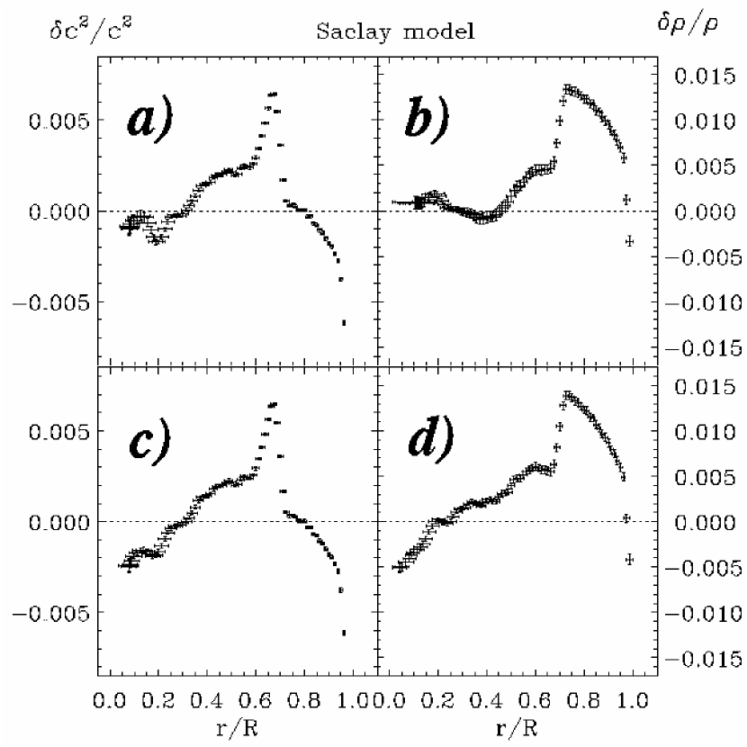
Figure 1: Sound speed and density inversion using a standard Saclay model (Brun et al. 1999). In these plots, panels a) and b) are obtained from the GOLF modes of l=0-2 above 1 mHz (Bertello et al. 2000a,b) and MDI medium-l data (l=3-250); the total number of modes is 2183. Panels c) and d) are obtained by adding three modes provided by Bertello et al. (2000b)(l=0, n=3,5,6) to the previous combination of p modes.

The results are presented in our figures in the form of the horizontal and vertical bars centered at the center of gravity of the localized averaging kernels. The size of the horizontal bars corresponds to a characteristic width (“spread”) of the averaging kernels and provides an estimate of the spatial resolution, and the vertical bars correspond to 1$\sigma$ formal error of the sound-speed and density corrections (see Table 1 of Turck-Chièze et al. 2001b). The standard solar model of Brun et al. (1999) was used as a reference. The inversion procedure was tested by using various other solar models as Sun’s proxy, and adding random Gaussian noise to calculated frequencies of these models to simulate the observational errors.

Figure 1 shows the inversions obtained for the sound speed and the density. This figure highlights how the low order modes impact deeply on the density profile and how they slightly improve the sound speed in the solar core. In the following, we shall call seismic model a model that reproduces as well as possible the observed sound speed profile. We will not take the density as a reference yet, since we first wait for confirmation of its profile by new detections at low frequencies, due to its extreme sensitivity to these modes. The density appears more sensitive to the detailed physics than the sound speed. It will be used in the future to progress on the dynamics of the Sun.

4 BUILDING THE SEISMIC MODELS

4.1 Starting Point

Figure 2: Upper figure: the contribution of the heavy elements to the opacity (plain curve). Superimposed is the profile of the Rosseland opacities $\kappa_{ross}$ (dot-dashed curve). Lower figure: number fraction of three elements related to the metal number fraction: the carbon (plain curve), the nitrogen (dashed curve), and the oxygen (dot-dashed curve). Solar composition at $4.6$ Gyr.

In this study, our goal is to cancel the discrepancy on $c_{s}$ between the solar models and the real Sun. To this end, we slightly modify a few physical parameters used in CESAM. Of course, we derive seismic models that are not unique: we could obtain similar results on the sound speed by adjusting different parameters. However, we justify our choices in section 4.3. We adjust the physical quantities the sound speed is sensitive enough to, and modify them within their error bars. It is decided to change as little parameters as possible.

We start from a specific solar model: the non-standard Btz model of Brun et al. (1999). This model was designed to reduce the discrepancy on $c_{s}$ between the standard models and the Sun at the BCZ, by taking into account the horizontal motion produced by the sudden disappearance of the differential rotation profile in the tachocline. Doing so, they get for the first time a correct $\mathrm{{}^{7}Li}$ abundance at the solar surface ($A_{\mathrm{{}^{7}Li}}=1.16\pm 0.10$ dex according to Grevesse & Noels 1993 [hereafter G&N93]): the only abundance that was not predictable before. It is a real improvement since the standard solar models do not consider any turbulent mixing at the BCZ. It is well known that the lithium is the only indicator of the internal structure for numerous stars and its abundance is very difficult to predict in classical stellar evolution. However, the adopted tachocline prescription is purely hydrodynamic and does not account for any magnetic field, eventhough the magnetic dynamo process is thought to occur in the thin tachocline.

The main impacts of this prescription are: to reduce the influence of the microscopic diffusion —the diffusion of heavy elements toward the center of the Sun is slowed down— and to burn $\mathrm{{}^{7}Li}$ on the main sequence. Three parameters define the tachocline:

• its current width, taken as $d=0.05R_{\odot}$;

• the Brünt-Väisälä frequency at the BCZ, $N=25\,\mu$Hz;

• the present rotation rate at the BCZ, $\Omega_{0}=415$ nHz.

Moreover, the turbulent diffusion coefficient in the tachocline is time-dependent, since it is related to the rotation rate. In the Btz model the rotation as a function of time follows the Skumanich’s law (Skumanich 1972).

4.2 The First Seismic Model: Seismic₁

Starting from Btz, we undertake the construction of a first seismic model (already presented in Turck-Chièze et al. 2001b). We focus primarily on the solar core where the energy generation and neutrino production occur: to adjust the physical parameters, we take advantage of our knowledge of the sensitivity of the model to the physical ingredients (through, for instance, Turck-Chièze & Lopes 1993; Dzitko et al. 1995; Turck-Chièze et al. 1997; Turck-Chièze et al. 2001a).

Figure 3: Seismic₁ model (plain curve with error bars) : a) difference in the square of the sound speed between the Sun and the model; b) difference in the density between the Sun and the model. The plain curves with no error bar are for the Saclay standard solar model, while the dashed curves are for the Btz model. Two other models based on seismic₁ are considered on the density figure: the model with the ${}^{3}He(^{4}He,\gamma)^{7}Be$ reaction rate reduced by $10\%$ (dot-dot-dot-dashed curve) and the model with the CNO poly-cycle reaction rates reduced by $70\%$ (dot-dashed curve) [From Turck-Chièze et al. 2001b].

We increase the $p-p$ cross section (hereafter $S(0)_{p-p}$) by $1\%$: usually $S(0)_{p-p}=4.00(1\pm 0.007^{+0.020}_{-0.011})10^{-22}$ keV b (Adelberger et al. 1998). As this cross section is only known theoretically, we try to constrain it by helioseismology. The change of $S(0)_{p-p}$ has a rather large impact on $c_{s}$. An increase of this cross section induces a decrease of the core temperature, since the model is calibrated to obtain the solar luminosity.

In parallel to this modification, we adjust the initial metallicity ($Z_{0}$) of the Sun. Compared to Btz ($Z_{0}=0.01959$), we increase it by $3.9\%$. In the radiative interior, a major contribution to the opacities comes from the heavy elements (see Fig. 2): at $0.6R_{\odot}$, about $85\%$ of the opacities are due to the metals. In the solar core, this part is still $45\%$, in this case all the elements are almost fully ionised, except iron. Actually, the opacities in the core are primarily due to inverse brehmstrahlung and electron scattering, while at $0.6R_{\odot}$ the bound-bound processes dominate. By increasing $Z_{0}$, we change both the Rosseland opacities ($\kappa_{ross}$) and the mean molecular weight ($\mu$), explaining why the sound speed of the seismic model decreases in the core and goes up in the radiative zone: in the core, the raise of $\mu$ dominates the raise in temperature produced by the increase of $\kappa_{ross}$; beyond $0.3R_{\odot}$, the raise in temperature overcomes the increase of $\mu$. A last change is carried out: the OPAL EOS is tabulated and depends on $Z_{0}$. Instead of $Z_{0}=0.01959$ used to compute the EOS table for Btz, we use a table computed with $Z_{0}=0.0203$. Actually, this change has no important impact on the sound speed profile.

Having reduced the discrepancy on $c_{s}$ in the radiative zone, we undertake to diminish it at the BCZ. To this end we modify the parameters defining the tachocline: we reduce its width from $0.05R_{\odot}$ to $0.025R_{\odot}$, in accordance with the most recent helioseismic results (e.g. Elliott et al. (1998) announce $d=0.02R_{\odot}$, Corbard et al. (1999) announce $d<0.05R_{\odot}$); we also increase the present rotation rate $\Omega_{0}$ from 415 to 430 nHz (Corbard et al. 1999). Moreover, to retrieve a good $\mathrm{{}^{7}Li}$ abundance at the surface, we increase the Brünt-Väisälä frequency $N$ from 25 to 105 $\mu$Hz. This frequency undergoes a dramatic change when approaching the convection zone. An increase of $N$ reduces the efficiency of the turbulent mixing and diminishes the $\mathrm{{}^{7}Li}$ depletion.

Another improvement is the change in the rotation law. Instead of the Skumanich’s law, which is far less realistic on the PMS, we utilize the law proposed by Bouvier et al. (1997), following Piau & Turck-Chièze (2001): the rotation rate of the Sun slightly goes down during the early evolution phase, and experiences a rapid acceleration at $10$ million years when the circumstellar accretion disk separates from the young Sun. Finally, the rotation rate decreases following the Skumanich’s law because of the magnetic breaking. Eventhough the impact of such a rotation law on the solar evolution is rather weak, its use is more realistic. To reach a correct $\mathrm{{}^{7}Li}$ content at $4.6$ Gyr, we suppose that the Sun was a slow rotator on the PMS (this is why we choose a disk separation at $10$ million years).

To complete the building of the seismic model, we concentrate on the outer part of the $\delta c_{s}^{2}/c_{s}^{2}$ profile: it is still far from flat, since no appropriate model exists for the upper layers with a 1D code. However, it is possible to obtain a better agreement with the Sun by calibrating the seismic model at a radius $R_{1}$ different from the standard one $R_{\odot}=6.9599\times 10^{10}$ cm deduced from photometric observations (e.g. Allen 1976). Recent analyses based on f-mode frequencies (e.g. Schou et al. 1997; Antia 1998) worked out seismic radii, respectively $R$ = 695.78 Mm and $R$ = 695.68 Mm, slightly smaller than the photometric one. This latter is greater than the recent optical determination $R$ = 695.51 Mm by Brown & Christensen-Dalsgaard (1998). There is neither a firm answer explaining the origin of these discrepancies, nor the effect of the solar cycle on the radius. Thus, we calibrate the seismic₁ model with $R_{1}=6.95936\times 10^{10}$ cm, with a consequent ad hoc improvement in the convective zone. Nevertheless, the inversion of the density and sound speed was carried out assuming the standard value for $R_{\odot}$.

The Table 1 lists all the main features of the models described in this paper. The seismic₁ model is also available on the web site http://apc-p7.org/Neutrino_APC/Sismic_model.html, with the detailed values of many parameters for a large number of shells (including the electron number density, see sect. 6.3).

4.3 Justification of the Changes for the Seismic₁ Model

The adjustments made increase the overall agreement between the Sun and the solar model on the $c_{s}$ profile (see Fig. 3). The improvement is less obvious when checking at the density profile but the progress is real too. To reach this improvement in the core and the radiative zone, we restricted the modifications to two parameters, $S(0)_{p-p}$ and $Z_{0}$. With such a restriction, it can be shown that we need to increase both these quantities to cancel (at least reduce) the discrepancy on $c_{s}$.

First, G&N93 work out $(Z/X)_{s}=0.0245\pm 10\%$ at the solar surface; this ratio has an impact on $Z_{0}$, whose value is larger than the present photospheric $Z$ value because of the microscopic diffusion. Let us suppose we want to cancel the sound speed difference by increasing $Z_{0}$ and reducing (or not changing) $S(0)_{p-p}$: to keep a $(Z/X)_{s}$ ratio within its error bar, we must limit the raise of $Z_{0}$ to $\approx 5.5\%$. This raise is lower than the one needed to cancel $\delta c_{s}^{2}/c_{s}^{2}$. Thus, if we increase $Z_{0}$, we also need an increase of $S(0)_{p-p}$ to get $\delta c_{s}^{2}/c_{s}^{2}=0$. Second, let us suppose we diminish $Z_{0}$: to cancel the sound speed difference in the core, we need to increase $S(0)_{p-p}$ beyond its upper error bar (equal to $2.0\%$).

Thus, the error bars on $S(0)_{p-p}$ and on $(Z/X)_{s}$ imply an increase of both parameters to cancel the discrepancy on $c_{s}$ below $0.6R_{\odot}$.

4.4 Non Uniqueness of the Seismic₁ Model: Alternative Seismic Models

Of course, the seismic₁ model is not unique:

First, we could have changed other nuclear cross sections instead of $S(0)_{p-p}$. Yet, Turck-Chièze et al. (2001a) highlight the lack of sensitivity of the sound speed to the other nuclear reactions, like $\mathrm{{}^{3}He(^{3}He,2p)^{4}He}$, $\mathrm{{}^{3}He(^{4}He,\gamma)^{7}Be}$ or the CNO bi-cycle. For instance, an increase of 25$\%$ for the first two reactions mentioned changes $\delta c_{s}^{2}/c_{s}^{2}$ by only $\approx 0.1-0.2\%$, and thus does not improve significantly the agreement with the Sun. On the other side, the sound speed is sensitive enough to the $p-p$ reaction rate. Therefore it seems more appropriate to only adjust $S(0)_{p-p}$: we build the best model with the most simple assumptions. On Fig. 3, you can see that the density is a little bit more sensitive to these reaction rates than the sound speed.

Second, with the accuracy reached on the sound speed, this quantity is sensitive to many physical parameters whose uncertainties can be quite large. It is primarily sensitive to $S(0)_{p-p}$, the opacities, the heavy element abundances, the microscopic diffusion process, but it can also undergo changes under “secondary” parameters such as the solar age or the solar radius.

4.4.1 The Seismic₂ Solar Model

Figure 4: Same caption as the previous figure for the seismic₂ model (left panels) and the seismic₃ model (right panels) (see text).

Actually, a second seismic model is constructed from Btz by modifying the opacities $\kappa_{ross}$, reducing $Z_{0}$ by $3.5\%$ and increasing $S(0)_{p-p}$ (we also calibrate this model to $R_{2}=6.95866\times 10^{10}$ cm). Its main advantage is to reach a $(Z/X)_{s}$ ratio equal to the one proposed by G&N93, while the one of the seismic₁ model approaches the upper limit of the error bar. By lowering $Z_{0}$ we reduce the mean molecular weight in the central part of the Sun, and the opacities as well. On the other side, we raise $\kappa_{ross}$ following Brun et al. (1998), by simulating an increase of about $7.5\%$ in the C, N, and O opacities. This raise could be attributed to uncertainties in the bound-bound and bound-free processes, i.e. to an intrinsic error in the opacity calculations. The change in the opacities of the CNO elements produces an increase of about $1.5\%$ in $\kappa_{ross}$ in the solar core, and about $4.5\%$ below the convection zone. This raise compensates for the decrease due to the reduction of $Z_{0}$, so that we get roughly: no opacity change in the core and an increase of about $1.5\%$ at $0.6R_{\odot}$. We just operate this ad hoc adjustment below $0.6R_{\odot}$ to diminish the discrepancy on $c_{s}$ at the BCZ. As for the first seismic model, we also need an increase of $S(0)_{p-p}$: by $1.3\%$. This seismic₂ model produces a sound speed profile similar to the one of the seismic₁ model, and even better at the BCZ (see Fig. 4).

However, for the rest of the paper, we just consider the seismic₁ model to derive the neutrino fluxes and to test the magnetic field: this model contains no ad hoc adjustment, less parameters were changed & the error bars on $S(0)_{p-p}$ and $Z_{0}$ (through the $(Z/X)_{s}$ ratio) are more or less well known while the uncertainties on $\kappa_{ross}$ remain unknown. However, the great effort done by laser measurements and the theoretical successes of the Livermore group lead to specific uncertainties on $\kappa_{ross}$ of the order of $5\%$.

4.4.2 The Opacities and the Change in Metal Abundances

Just a few words about these opacities: the OPAL95 tables we use to interpolate the $\kappa_{ross}$ values were calculated assuming a G&N93 mixture. Along the solar evolution the metal composition in the core changes: because of the CNO poly-cycle and the microscopic diffusion, the relative number fractions of the metals are modified (see Fig. 2 for the composition at $4.6$ Gyr). This should have an impact on the opacities: we have to correct them as soon as the solar core composition is “far” from the G&N93 mixture (this occurs at an age of, roughly, 100 million years). Starting from the seismic₁ model, we compute a very similar model but with a correction for $\kappa_{ross}$ below $0.15\,R_{\odot}$ to take into account the change in the composition. Actually, this correction is very small: from $-0.88\%$ at $0R_{\odot}$ to $-0.5\%$ at $0.15R_{\odot}$, for the Sun at $4.6$ Gyr. It has a minute impact on the sound speed profile: it just increases $\delta c_{s}^{2}/c_{s}^{2}$ by $0.0005$ in the core! However, with the precision we reach on $c_{s}$, we can test such a small effect. This latter leads to that, instead of increasing $S(0)_{p-p}$ by $1\%$ for the seismic₁ model, an increase by only $0.75\%$ is enough.

4.4.3 The Impact of the Age: Seismic₃

Finally, we also check the sensitivity of $c_{s}$ to the solar age ($t_{\odot}$). A recent work by Dziembowski et al. (1999) used helioseismology to determine $t_{\odot}$. Depending on the method they use, they derive very different results. However, using the small frequency separation which they claim to be the most accurate measure, they conclude that $t_{\odot}=4.66\pm 0.11$ Gyr (the lifetime on the PMS must be added). Starting from Btz, we compute the seismic₃ model: those are basically the same models except that $t_{\odot}=4.735$ Gyr for the second one, the tachocline parameters are changed (as for the previous seismic models), and we calibrate at $R_{2}$. The augmentation by only $\approx 2.9\%$ of $t_{\odot}$ produces a rather important change in the $c_{s}$ profile and reduces the discrepancy with the Sun, eventhough the reduction is less significant than with the other seismic models (see Fig. 4). The seismic₃ model shows that, supposing we under-estimate the solar age, an increase of $S(0)_{p-p}$ and $Z_{0}$ less important is needed to retrieve the flat $\delta c_{s}^{2}/c_{s}^{2}$ profile of the seismic₁ model. Eventhough this does not challenge the need to raise both $S(0)_{p-p}$ and $Z_{0}$, this reduces the amplitude of the increase. On the contrary, a solar age less than $4.6$ Gyr would favor a larger increase of the two parameters. It is noticeable that the density profile greatly disfavors the seismic₃ model (see Fig. 4, right figure, panel b), unlike the sound speed profile.

Table 1: Main Features of the Solar Models

	Btz	Seismic1	Seismic2	Seismic3	Seismic1B1	Seismic1B11
Age (Gyr)	4.6	4.6	4.6	4.735	4.6	4.6
Radius ($10^{10}\,\mathrm{cm}$)	6.9599	6.95936	6.95866	6.95866	6.95866	6.95866
$X_{0}$	0.70817	0.70377	0.70663	0.70958	0.69193	0.70081
$Z_{0}$	0.01959	0.02035	0.01893	0.01959	0.02035	0.02035
$(Z/X)_{0}$	0.02766	0.02892	0.02679	0.02761	0.02942	0.02904
$\alpha$	1.755	1.934	1.751	1.776	1.753	1.770
$(Z/X)_{s}$	0.0255	0.02628	0.02449	0.02521	0.02684	0.02654
$Y_{s}$	0.2508	0.2508	0.2507	0.2470	0.2631	0.2549
$\mathrm{{}^{7}Li}$ (dex)	1.14	1.10	NR	NR	NR	NR
d ($R_{\odot}$)	0.05	0.025	0.025	0.025	0.025	0.025
N ($\mu$Hz)	25	105	45	45	45	45
$\Omega_{0}$ (nHz)	415	430	430	430	430	430
BCZ ($R_{\odot}$)	0.7142	0.7115	0.7144	0.7121	0.7137	0.7122
$\mathrm{{}^{71}Ga}$ (SNU)	127.1	128.0	125.9	127.9	135.1	129.8
$\mathrm{{}^{37}Cl}$ (SNU)	7.04	7.47	7.11	7.47	8.88	7.81
$\mathrm{{}^{8}B}$ ($10^{6}\,\mathrm{cm^{-2}\,s^{-1}}$)	4.98	4.98	4.71	4.98	6.04	5.23
Atm	H	K	H	H	H	H

4.5 Constraints Suggested by the Seismic Models

In the previous sections we emphasize the sensitivity of $c_{s}$ to a large set of parameters used to work out different seismic models: that makes it difficult to draw firm conclusions concerning the changes in just a few parameters, since these modifications cannot be proved to be the unique solution. However, under the assumption that the major uncertainties in the solar models (for the core and radiative zone) are due to some reaction rates, the metallicity and the opacities, our seismic models shed new lights on these physical quantities.

First, the different seismic models we computed all favor a slight increase in the $S(0)_{p-p}$ factor: from $0.75\%$ to $1.3\%$ depending on the model. The strong influence of the $p-p$ reaction was known for a long time (Turck-Chièze & Lopes 1993) and a raise was also recently proposed by Antia & Chitre (1998). However, the increase we work out is less than theirs (due to the data improvement) and could be even less if the solar age turned out to be slightly larger than $4.6$ Gyr (on the contrary, a lower age implies a larger increase of $S(0)_{p-p}$). Incidentally, this result confirms that the calculations of $S(0)_{p-p}$ are quite good despite their purely theoretical base.

Figure 5: Weighted difference between the p mode frequencies of the seismic₁ model and the observed frequencies. These latter are the one of GOLF for $\ell\leq 3$ (García et al. 2001 and Bertello et al. 2000a), and the one of MDI for $\ell>3$ (Rhodes et al. 1997).

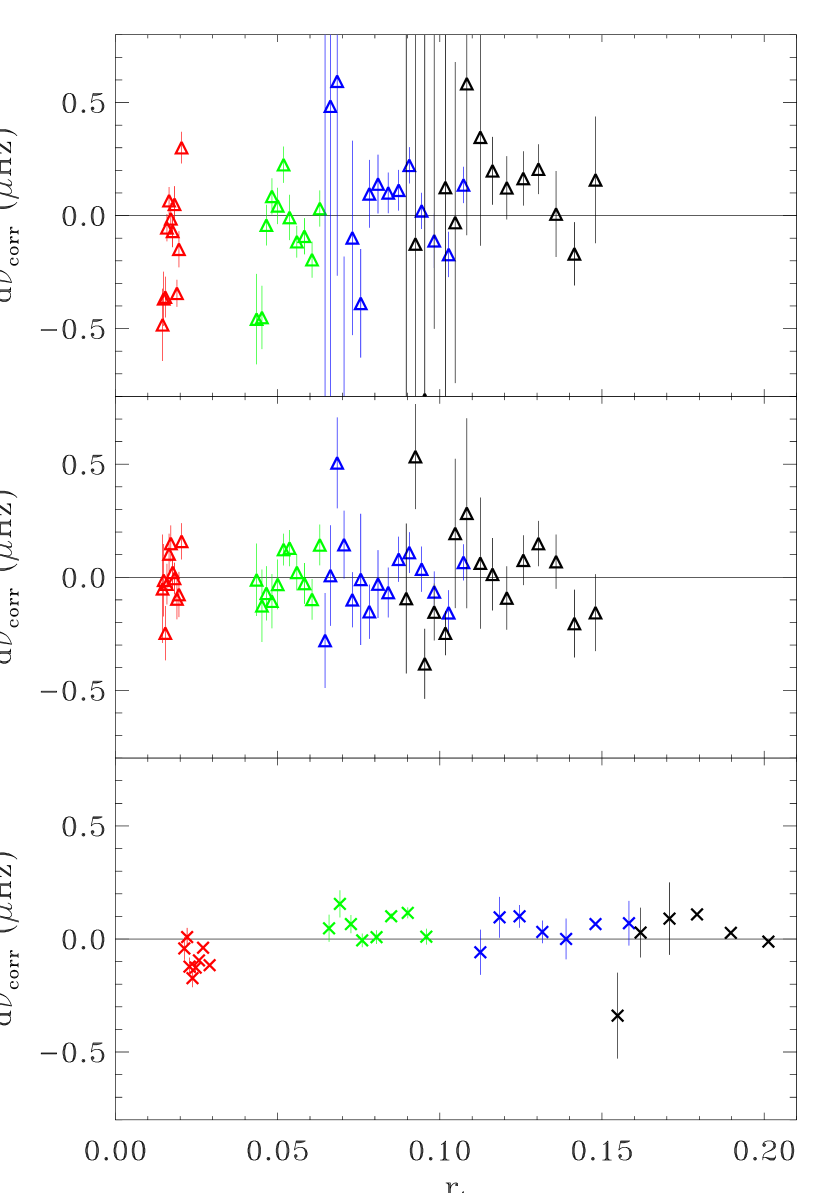
Figure 6: Difference between the p mode frequencies of the seismic₁ model and the observed frequencies from GOLF, as a function of the internal turning point. In the upper figure: we have used the frequencies of Lazrek et al. (1997). In the middle and lower figures: García et al. (2001) and Bertello et al. (2000a). For the upper and middle figures we show the modes with $n\geq 15$, for the lower figure we show $n\leq 14$. We have corrected the frequency differences by the usual $Q_{nl}$ factors, and by removing the surface effects (we fitted the slope by a polynomial). Color code: the red symbols are for $\ell=0$, the green ones for $\ell=1$, the blue for $\ell=2$, and the black for $\ell=3$.

Concerning $Z_{0}$, an increase by $3.9\%$ is strongly favored by the seismic₁ model, while the seismic₂ model shows that an increase of $\kappa_{ross}$ combined with a decrease of $Z_{0}$ yields the same result in terms of $c_{s}$. Since either solutions are acceptable, we cannot favor the increase or decrease of $Z_{0}$. Opacities and heavy element abundances are closely related, and part of the error bars on $\kappa_{ross}$ are due to the uncertainty on $Z$.

However, this change by almost $4\%$ in $Z$ is far from trivial if you consider that the microscopic diffusion changed $Z$ by only $10\%$ since the beginning of the hydrogen burning. Actually, the need to increase $Z_{0}$ —in the seismic₁ model— could be the manifestation of some forgotten hydrodynamic phenomenon. The use of both the density and rotation profiles in the core may help to solve this point. Gravity modes may also be helpful. For now, we only have a static view of the radiative region (contrary to the convective one). For instance, we cannot introduce the history of the angular momentum in the stellar equations: therefore, it seems that only hydrodynamical simulations will be able to reproduce the real Sun. Nevertheless, the present analysis tends toward a reduced effect on the neutrino prediction when we do not correctly simulate the dynamical phenomena. Thus, this static view of the Sun remains an astrophysical problem that could have a larger impact on other stars.

Concerning $t_{\odot}$, the sound speed and density profiles change in an opposite way: while a raise in $t_{\odot}$ reduces the discrepancy on $c_{s}$ below $0.2R_{\odot}$, it increases it for $\rho$. If we refer to the density profile, which is more sensitive, it seems that $t_{\odot}=4.6$ Gyr is a satisfactory value for the solar age (the value needed to best reduce the discrepancy on $\rho$ below $0.6R_{\odot}$ is $4.55$ Gyr). Moreover, an augmentation of $t_{\odot}$ is strongly disfavored by the density, while the sound speed does not rule it out (but does not strongly support it too).

Finally, it seems that calibrating the solar models to a radius slightly smaller than the usual one (by 50-125 km, this value depends on the atmosphere model) improves the agreement between the Sun and the models above $0.9\,R_{\odot}$.

5 THE OSCILLATION FREQUENCIES

An important result of the solar models is the computation of the oscillation frequencies for the p and g modes. We use the seismic₁ model: it was derived using the MHD EOS (Mihalas, Däppen & Hummer 1988) and the k5777 $T(\tau)$ law (derived from a Kurucz’s model) for the atmosphere model (with a reconnection at $\tau$ = $20$ following Morel et al. (1994)). This is an improvement in comparison with our previous Btz model using the $T(\tau)$ Hopf’s law, with the CEFF EOS (Christensen-Dalsgaard & Däppen 1992).

The Figure 5 shows the difference —scaled by the usual $Q_{n,l}$ factors— between the theoretical and the observed p-mode frequencies, up to $\ell=200$, versus the inner turning point $r_{t}$ expressed as:

$$\frac{w^{2}+4\pi G\rho}{c_{s}^{2}}=\frac{L^{2}}{r_{t}^{2}}$$ (1)

$w$ is the mode frequency, $G$ the gravity constant and $L=(\ell+0.5)$ with $\ell$ the mode degree. We have taken the self-gravity of plane acoustic waves into account.

As usual, there is a very good agreement for frequencies smaller than 2 mHz and a worse one at larger frequencies, mainly due to the difficulty to model the turbulent surface. The Table 2 gives the frequencies of the low degree g modes.

The Figure 6 details the quality of the seismic data we use by showing the weighted difference between calculated and observed frequencies, as a function of the internal turning point. The surface effect has been removed by a polynomial fit of the general trend above 2.2 mHz. We separate the modes in two ranges: in the first two figures we draw modes with $n>14$ and in the third one, those with $n\leq 14$. It appears clearly that the use of the higher frequency domain is not disfavored by the general trend previously observed. The real difficulty comes from the stochastic excitation and the mode correlated lifetime. This leads to a bad determination of the frequencies after 8 months of measurement (Fig. 6a). The situation is improved by a longer integration time (here 1290 days) (Fig. 6b) but it is obvious that the comparison computed/observed frequencies is better when we access to the low frequency range ($n<15$ or $\nu<2.2$ mHz). In this case, the modes have a longer lifetime and an insight into the very central core (which is important for high energy neutrino fluxes) could be obtained with a large increase of the sensitivity. Therefore, the inversion of the sound speed is better determined (even if the use of the sole low order modes reduce the radial accuracy), as for the density profile. This is natural since we also reach the modes that have a mixed gravity and acoustic character.

Table 2: G-mode Frequencies with the Seismic₁ Model

$\ell$	$n$	$\nu$ ($\mu$Hz)	$\ell$	$n$	$\nu$ ($\mu$Hz)	$\ell$	$n$	$\nu$ ($\mu$Hz)	$\ell$	$n$	$\nu$ ($\mu$Hz)	$\ell$	$n$	$\nu$ ($\mu$Hz)
1	-6	95.47	3	-16	93.12	4	-13	136.49	5	-14	150.83	6	-17	147.70
1	-5	109.28	3	-14	104.21	4	-12	145.31	5	-13	159.55	6	-15	162.42
1	-4	127.79	3	-13	110.84	4	-11	155.27	5	-12	169.27	6	-14	170.87
1	-3	153.25	3	-12	118.37	4	-10	166.60	5	-11	180.14	6	-13	180.19
1	-2	191.55	3	-11	126.96	4	-9	179.62	5	-10	192.39	6	-12	190.49
1	-1	262.73	3	-10	136.85	4	-8	194.59	5	-9	206.31	6	-11	201.94
2	-11	94.91	3	-9	148.33	4	-7	211.92	5	-8	222.13	6	-10	214.69
2	-10	102.68	3	-8	161.72	4	-6	231.62	5	-7	240.19	6	-9	229.05
2	-9	111.82	3	-7	177.46	4	-5	250.39	5	-6	260.12	6	-8	245.20
2	-8	122.63	3	-6	195.93	4	-4	265.08	5	-5	272.04	6	-7	263.41
2	-7	135.59	3	-5	217.07	4	-3	291.42	5	-4	288.27	6	-6	283.04
2	-6	151.26	3	-4	238.35	4	-2	328.10	5	-3	316.38	6	-5	289.06
2	-4	194.06	3	-3	261.31	4	-1	368.29	5	-2	350.90	6	-4	308.82
2	-3	222.02	3	-2	296.50	5	-17	129.44	5	-1	385.55	6	-3	335.81
2	-2	256.09	3	-1	340.07	5	-16	135.89	6	-19	135.32	6	-2	367.39
2	-1	296.38	4	-14	128.64	5	-15	142.98	6	-18	141.25	6	-1	396.69

Figure 7: Neutrino production as a function of the fractional radius. In the upper figure, we have drawn the p-p (plain curve), $\mathrm{{}^{8}B}$ (dot-dashed curve), $\mathrm{{}^{7}Be}$ (dashed curve), and the pep (dot-dot-dot-dashed curve) neutrinos. In the lower figure, the $\mathrm{{}^{13}N}$ (plain curve), $\mathrm{{}^{15}O}$ (dashed curve), and $\mathrm{{}^{17}F}$ (dot-dashed curve) neutrino production is shown. For each neutrino “type”, we have drawn $(1/F_{t})\,(dF/dr)$ where $F$ is the flux in $\mathrm{s^{-1}}$, $r$ the fractional radius, and $F_{t}$ the total flux for this neutrino type (integrated over the entire Sun).

6 SEISMIC PREDICTED NEUTRINO FLUXES

6.1 The Solar Neutrino Predictions

Since the neutrino production is not pointlike, the precise calculation of the expected emitted $\nu_{e}$ flux requires to know where the neutrinos are produced. The Figure 7 recalls the production zones for the p-p, pep, $\mathrm{{}^{8}B}$, $\mathrm{{}^{7}Be}$, $\mathrm{{}^{13}N}$, $\mathrm{{}^{15}O}$ and $\mathrm{{}^{17}F}$ neutrino fluxes. As it clearly appears on the figure, most of them depend on the very central part. Now we recall that the first radius we have for the sound speed is at $0.07\pm 3.6\%R_{\odot}$ (Table 1 of Turck-Chièze et al. 2001b), and only gravity modes may improve this situation.

Neutrino predicted fluxes have been calculated for the three seismic models (see Table 1). We may note that they do not differ significantly. Moreover, they are only slightly different from our previous predictions in Brun et al. (1999) or from the recent solar models (e.g. Bahcall et al. 2001). This is logical since the last modifications we introduced are minor. In Turck-Chièze (2001), we recall the progress made to stabilize these fluxes. Detailed neutrino capture predictions are shown for the seismic₁ model (see Table 3).

The present predictions are of great interest (in comparison with those obtained ten years ago) since they include helioseismic data that validate the updated physics at the needed level (see Table 2 of Turck-Chièze et al. 2001a). The emitted neutrino fluxes we predict are not only theoretical but also partly deduced from precise seismic “observations” of the solar core, and they confirm the discrepancy between predictions and detections, favouring the neutrino flavor transformation. The next step is to sum the fluxes of these different flavors received on Earth. Such data are now available thanks to the SNO experiment.

Table 3: Neutrino Fluxes of the Seismic₁ Model

	pp	pep	$\mathrm{{}^{7}Be}$	$\mathrm{{}^{8}B}$	$\mathrm{{}^{13}N}$	$\mathrm{{}^{15}O}$	$\mathrm{{}^{17}F}$
Sun	1.673$\times\,10^{38}$	3.936$\times\,10^{35}$	1.372$\times\,10^{37}$	1.408$\times\,10^{34}$	1.631$\times\,10^{36}$	1.404$\times\,10^{36}$	8.718$\times\,10^{33}$
Earth	5.916$\times\,10^{10}$	1.392$\times\,10^{8}$	4.853$\times\,10^{9}$	4.979$\times\,10^{6}$	5.767$\times\,10^{8}$	4.967$\times\,10^{8}$	3.083$\times\,10^{6}$
$\mathrm{{}^{71}Ga}$	69.34	2.840	34.79	11.95	3.483	5.648	3.512$\times\,10^{-2}$
$\mathrm{{}^{37}Cl}$	0.000	2.228$\times\,10^{-1}$	1.155	5.676	9.573$\times\,10^{-2}$	3.283$\times\,10^{-1}$	2.057$\times\,10^{-3}$
Capture Predictions for
$\mathrm{{}^{71}Ga}$ : $128.1\pm 8.9$ SNU, $\mathrm{{}^{37}Cl}$ : $7.48\pm 0.97$ SNU, water experiments : $4.98\pm 0.73\,\times 10^{6}$ $\mathrm{cm^{-2}\,s^{-1}}$

6.2 Comparison of the $\mathrm{{}^{8}B}$ Emitted Flux with the SNO & Superkamiokande Results

Ahmad et al. (2001) announced the first results of the SNO collaboration on charged current (CC) and elastic scattering off electrons (ES) reactions.

The CC reaction is only sensitive to electron-type neutrinos, while the ES reaction, also measured in the Superkamiokande experiment, is sensitive to all flavors. The measured $\mathrm{{}^{8}B}$ neutrino fluxes for the CC and ES reactions are:

$$\Phi^{CC}_{SNO}(\nu_{e})=1.75\pm 0.07({stat.})^{+0.12}_{-0.11}({sys.})10^{6}\mathrm{cm^{-2}s^{-1}}$$

$$\Phi^{ES}_{SNO}(\nu_{x})=2.39\pm 0.34({stat.})^{+0.16}_{-0.14}({sys.})10^{6}\mathrm{cm^{-2}s^{-1}}$$

The present statistical error on the elastic scattering is still large and the sensitivity to the $\nu_{\mu}$, $\nu_{\tau}$ or anti $\nu_{\mu}$, $\nu_{\tau}$ (only $16\%$ in comparison to $100\%$ for $\nu_{e}$) is low. Therefore, it is not possible yet to properly extract the different flavors from the SNO experiment alone, despite the difference in the two measured fluxes. Fortunately, the ES result is in agreement with the measure from the SK experiment (Fukuda et al. 2001):

$$\Phi^{ES}_{SK}(\nu_{x})=2.32\pm 0.03({stat.})^{+0.08}_{-0.07}({sys.})10^{6}\mathrm{cm^{-2}s^{-1}}$$

This flux is equal to $\simeq 47-48\%$ of the seismic₁ model $\mathrm{{}^{8}B}$ neutrino prediction (Turck-Chièze et al. 2001b):

$$\Phi(\nu_{x})=4.98\pm 0.73\times 10^{6}\mathrm{cm^{-2}s^{-1}}$$

It is widely known that the $\mathrm{{}^{8}B}$ neutrino flux is the most difficult to predict and is very dependent on the physics of the core. A fundamental improvement achieved by the seismic model is the reduction of the error bars in the neutrino prediction, through the reduction of the uncertainty on the $p-p$ reaction rate, the $(Z/X)_{s}$ ratio… This point has already been discussed in the Table 2 of Turck-Chièze et al. (2001b) that gives the detailed uncertainties on neutrino predictions. We point out that the neutrino fluxes derived here are not only “observational” (to a certain extent) but are also affected by reduced uncertainties. They also include the recent rejection of several astrophysical solutions to the neutrino puzzle proposed in the past.

Nevertheless, the $S(0)_{17}$ factor has no impact on the structure and was badly determined more than 4 years ago (see Turck-Chièze 2001). For instance, Adelberger et al. (1998) propose $S(0)_{17}=19^{+4}_{-2}$ eV b. But the experimental measurements have been largely improved. In our models, we use the value of Hammache et al. (1998) of $18.5\pm 1$ eV b. Unfortunately, the recent result of Junghans et al. (2002) of $22.3\pm 0.7$ eV b, is only marginally in agreement with the previous one. Thus the uncertainty on the present predicted neutrino flux, including the one of the seismic₁ model, could be a bit larger today.

Actually, the major result of the last year is the one obtained by the SNO collaboration when they add the estimated number of detected muon and tau type neutrinos to the electronic ones (using the SK results); they find:

$$\Phi(\nu_{x})=5.44\pm 0.99\times 10^{6}\mathrm{cm^{-2}s^{-1}}$$

a result very consistent with the previous value validated by the present helioseismic data.

This strongly favors or even “proves” the existence of neutrino oscillations: a part of the $\nu_{e}$ must be converted into $\nu_{\mu}$ and $\nu_{\tau}$, as far as new seismic results do not lead to other conclusion. Actually the present study stays in the framework of a static solar core, with classical phenomena. This representation is compatible with the present seismic results but we still need to extract the rotation and magnetic field in the radiative zone to check this assumption.

6.3 The Neutrino Oscillation Related Quantities

Figure 8: Upper figure: the electron number density for the seismic₁ model. The approximation proposed by Bahcall (for instance Bahcall et al. 2001) has also been drawn (dashed curve). Lower figure: the neutron number density for the seismic₁ model (we show the $n_{e}/n_{n}$ ratio).

6.3.1 The Electron Number Density

Following this framework, a part of the neutrino oscillations could be explained by the well-known Mikheyev-Smirnov-Wolfenstein effect (MSW effect, see e.g. Mikheyev & Smirnov 1986): an electron type neutrino may undergo a resonant oscillation in the Sun and then be converted into a muon or tau type neutrino. This effect assumes that the neutrinos have masses and that the flavor eigenstates are different from the mass eigenstates.

For the sake of simplicity, we suppose two flavors ($\nu_{e}$ and $\nu_{\mu}$) and two mass eigenstates ($\nu_{1}$ and $\nu_{2}$). We assume that $\nu_{1}$ is close to $\nu_{e}$, and $\nu_{2}$ is close to $\nu_{\mu}$. When an electron type neutrino is created in the solar core, the flavor eigenstates are almost “propagation eigenstates”, because of the high electron number density ($n_{e}$). But during the propagation from the neutrino toward the solar surface, $n_{e}$ decreases and the flavor states are no more propagation eigenstates: the neutrino state vector starts to oscillate around the new propagation eigenstate. This latter changes with the further decrease of $n_{e}$, and gets closer to $\nu_{2}$ (initially, it was close to $\nu_{e}$). Depending on the variation of $n_{e}$, this change is more or less rapid and said adiabatic or not. In the case of an adiabatic change, the probability for an emitted electron type neutrino to be detected as a muon type neutrino at the solar surface is rather simple to calculate. In the non-adiabatic case, the conversion probability is more tricky to work out. In both cases, the electron number density is needed with a high accuracy all along the solar radius, to compute the conversion probabilities.

Therefore, we derive $n_{e}$ for the seismic₁ model. To do so, we use the precise mass fractions returned by CESAM: we know the mass fractions for the $\mathrm{{}^{1}H}$, $\mathrm{{}^{2}H}$, $\mathrm{{}^{3}He}$, $\mathrm{{}^{4}He}$, $\mathrm{{}^{7}Li}$, $\mathrm{{}^{7}Be}$, $\mathrm{{}^{9}Be}$, $\mathrm{{}^{12}C}$, $\mathrm{{}^{13}C}$, $\mathrm{{}^{14}N}$, $\mathrm{{}^{15}N}$, $\mathrm{{}^{16}O}$, & $\mathrm{{}^{17}O}$ chemical elements, plus an extra element (with $A=28$ and $Z=13$), as a function of the fractional radius. We just have to derive the number fractions of all these elements, and multiply these number fractions by the electron number of the corresponding chemical element. By adding all the terms we obtained this way, we determine the electon number density as a function of the radius. The result is drawn in the upper part of Fig. 8.

6.3.2 The Neutron Number Density

If the neutrino has a magnetic moment (either a dipole or/and transition moments), it might interact with the solar magnetic field. Provided that the magnetic moment and the magnetic field are large enough, this field could flip the spin of the neutrino: a left-handed neutrino could become right-handed. Moreover, the possible flavor transition magnetic moments could result in a spin-flavor precession: the neutrino could change both its chirality and its flavor. This double precession could be matter-enhanced through the interactions of neutrino with the electrons, protons and neutrons: this is the Resonant Spin-Flavor Precession process (RSFP, e.g. Lim & Marciano 1988). To compute the conversion probabilities for the RSFP, the neutron number density $n_{n}$ is needed (see the lower part of Fig. 8): we derive it the same way as the electon number density, but instead of using the electron number of each chemical element, we use its neutron number. It is important to note that both the MSW and RSFP processes could cohabit inside the Sun.

The detailed $n_{e}$ and $n_{n}$ profiles are available with the seismic₁ model on the web site whose address was previously mentioned, in order to calculate quantities related to the neutrino oscillations.

7 UNSOLVED PROBLEMS IN THE SEISMIC MODELS

Despite the overall agreement in the sound speed between the Sun and the seismic models below $0.6R_{\odot}$, two regions of our star remain poorly described: the tachocline region and the upper layers, both are expected to undergo dynamic effects. Moreover the central rotation law is not taken into account in this analysis (Garcia, R. A., Couvidat, S., Turck-Chièze, S. et al., in preparation).

In the superadiabatic region it is well known that the turbulent pressure becomes non negligible compared to the gas pressure. Moreover, the tachocline and the upper solar layers are shear layers in which rotation rates change rapidly (e.g. see the rotation curve of Howe et al. 2000). A 1D stellar evolution code cannot afford an efficient treatment of these dynamic regions. Neither the rotation of the Sun nor its magnetic field are taken into account, whereas it is widely thought that the tachocline is the base of the magnetic dynamo process. Of course, the neutrino emission and the solar core physics are rather insensitive to the tachocline and beyond, but the neutrino behaviour may depend on these layers. Progresses are needed to connect interior phenomena related to these neutrinos, to what is observed out of the star. If the neutrinos have a magnetic moment, they could interact with the solar interior magnetic field. In the next section we focus on the solar large-scale magnetic field: we add magnetic pressure and derive new solar models.

7.1 The Magnetic Field Tested by the Sound Speed

The goal of this analysis is to test the sensitivity of $c_{s}(r)$ to the magnetic field and constrain the amplitude of this field. We also check (and use) the sensitivity of the density.

Basically, the presence of a magnetic field changes the wave velocity in two ways:

• it changes the gas pressure because of the hydrostatic equilibrium;

• it adds a part of the Alfvén speed $v_{a}=B^{2}/(4\pi\rho)$ (in cgs units) to the wave velocity.

Thus, any magnetic field should be imprinted in the “magneto-acoustic” wave velocity. Of course, the 3D structure of the field is of great importance since the angle between the field lines and the seismic waves determines the way these latter are accelerated: the wave velocity is no more an isotropic quantity. Unfortunately, we cannot account for the field structure with a 1D stellar code, and so we just add a magnetic pressure term $P_{mag}$ in the stellar structure equations: $P_{mag}=B^{2}/(8\pi)$ (in cgs units). Therefore, the basic hydrostatic equilibrium equation is changed into:

$$\frac{dP_{gas}}{dm}=-\frac{GM}{4\pi r^{4}}-\frac{dP_{mag}}{dm}$$ (2)

The main problem is to choose an appropriate magnetic field $\bf{B(r)}$ for the solar interior, since little is known about the inner field. Roughly speaking, it seems that large scale magnetism may be important in three regions: the radiative zone, the tachocline, and just below the solar surface.

7.2 Origin of a Large Scale Magnetic Field

Parker presented the hydromagnetic dynamo theory for the Sun in 1955. The $\alpha-\omega$ kinematic dynamo needs both differential latitudinal rotation (parameter $\omega$) and turbulent —cyclonic— movements (parameter $\alpha$). The differential rotation produces a toroidal magnetic field from a poloidal one, while the cyclonic movements slow down the lift and twist of this toroidal field which has enough time to get amplified. The lift of the field is due to the magnetic buoyancy, while the twist results from the Coriolis force. Both these actions induce a poloidal field from the toroidal one, thus restoring the initial field. This basic picture has been widely reviewed as different dynamo processes were developped and improved. For instance, let us mention the Babcock-Leighton dynamo models that regenerate the poloidal field by the eruption of the toroidal field at the solar surface (e.g. see Durney 1997 for a modified Babcock-Leighton dynamo analysis). It is now commonly believed that the seat of the (main) solar dynamo process is the tachocline. A small seed poloidal field —a legacy of the PMS evolution— in the radiative interior should have given birth to a magnetic field with poloidal and toroidal components. Although this scenario seems widely accepted, the situation is rather confused when going into details. The seat of the poloidal field regeneration is not located, it could be the tachocline (as is induced by the “Parker” dynamo process), or just below the solar surface (as proposed by the Babcock-Leighton dynamo). Moreover, it is unclear whether or not the toroidal part of the field prevails in the solar interior: the surface activity proves that the toroidal field is larger than the poloidal one in the upper layers of the Sun, but only a few clues of what happens in the deep interior are known. We just consider toroidal fields in this paper.

7.3 Simulated Magnetic Profiles

Following Dzitko (1995) we simulate fields as:

Figure 9: Magnetic fields simulated: in the radiative interior (plain curve), in the tachocline (dashed curve), in the upper layers (dot-dashed curve). The amplitudes of the fields have been normalized.

$$\mathbf{B_{\phi}}=a(r)\frac{d}{d\theta}P_{k}(cos\theta)\,\mathbf{e_{\phi}}$$ (3)

With the spherical coordinates $(r,\theta,\phi)$. $P_{k}(cos\theta)$ is a Legendre polynomial of degree $k$.

For argument’s sake, we assume $k=2$, meaning that the field is quadrupolar (in accordance with the surface-magnetism manifestations). The presence of a magnetic pressure modifies in a direct way the wave velocity: we must take into account the Alfvén speed. Since we are only interested in the radial velocity and a toroidal field is perpendicular to the radial direction, the new wave velocity is $\sqrt{c_{s}^{2}+v_{a}^{2}}$ (on the figures, we continue to note this quantity “$c_{s}$” for convenience, eventhough it is no more the sound speed, strictly speaking). For the function $a(r)$, two profiles are considered, following Gough & Thompson (1990).

First, to simulate a magnetic field in the radiative zone, we choose:

$$a(r)=\left\{\begin{array}[]{ll}K_{\lambda}(\frac{r}{r_{0}})^{2}(1-(\frac{r}{r_{0}})^{2})^{\lambda}&\textrm{if $r\leq r_{0}$}\\ 0&\textrm{otherwise}\end{array}\right.$$ (4)

With $K_{\lambda}=(1+\lambda)(1+1/\lambda)^{\lambda}\,B_{0}$, $r_{0}=0.712R_{\odot}$ being approximately the BCZ and $\lambda=10r_{0}+1$. $B_{0}$ —the highest intensity of the field— is set to different values (see Table 4). The addition of the magnetic pressure is made when the Sun enters the ZAMS. The intensities of these fields are very high, compared to the prediction of Gough & MacIntyre (1998) who claim for a (poloidal) field with an amplitude of $\approx 0.1$ T in the deep interior. Moreover, the virial theorem rules out fields larger than $\approx 10^{4}$ T (Mestel & Weiss 1987). The maximum values of the $P_{mag}/P_{gas}$ ratio (hereafter $\beta^{-1}$) are available in Table 4, for all the models discussed here. We could also give the $v_{a}/c_{s}$ ratio, but $\beta$ and this ratio are closely related: $v_{a}/c_{s}=\sqrt{2/(\beta\,\Gamma_{1})}$. Both contributions of the magnetic field to the change in $c_{s}$ — the indirect change through the modification of the solar structure, and the direct change through the addition of $v_{a}$— depend on the $\beta$ values.

Second, we also utilize as $a(r)$ profile:

$$a(r)=\left\{\begin{array}[]{ll}B_{0}(1-(\frac{r-r_{0}}{d})^{2})&\textrm{if $|r-r_{0}|\leq d$}\\ 0&\textrm{otherwise}\end{array}\right.$$ (5)

Table 4: Models with Magnetic Field

Name	$B_{0}$ (T)	Center ($R_{\odot}$)	$(P_{mag}/P_{gas})_{max}$
seismic1B1	$10^{4}$	$0.236$	$2.85\times 10^{-2}$
seismic1B11	$5\times 10^{3}$	$0.236$	$6.96\times 10^{-3}$
seismic1B12	$3\times 10^{3}$	$0.236$	$2.49\times 10^{-3}$
seismic1B13	$1\times 10^{3}$	$0.236$	$2.80\times 10^{-4}$
seismic1B2	$30$	$0.712$	$6.15\times 10^{-5}$
seismic1B21	$50$	$0.712$	$1.71\times 10^{-4}$
seismic1B3	$2$	$0.96$	$1.34\times 10^{-4}$
seismic1B31	$3$	$0.96$	$3.02\times 10^{-4}$

With $d$ the half-width of the zone with a magnetic field, and $r_{0}$ its center. To simulate a magnetic field in the tachocline, parameters are set to: $d=0.02R_{\odot}$ and the radius $r_{0}$ of transition between radiative and convective zones varies along the solar evolution. We set $B_{0}$ to $30$ T according to Antia et al. (2000) for the seismic₁B₂ model, and $50$ T for the seismic₁B₂₁ model.

Finally, this profile is also used to simulate a possible field in the upper solar layers. Such a field was hinted by Antia et al. (2000) from an analysis of the Global Oscillation Network Group (GONG) and MDI data. To test a field anchored at $0.96R_{\odot}$, parameters are set to $r_{0}=0.96R_{\odot}$ and $d=0.035R_{\odot}$. $B_{0}$ is set to $2$ (the value proposed by Antia et al. 2000) and $3$ T. The fields at the BCZ and in the upper layers are both added at $85$ million years, when the solar core is no more convective.

Figure 10: Upper figure: difference in the gas pressure between the seismic₁B₁ and the seismic₁ models (thin plain curve). Same figure for the seismic₁B₁₁ (dashed curve), the seismic₁B₁₂ (dot-dashed curve), and the seismic₁B₁₃ (dotted curve) models. Superimposed is the difference in the temperature between the seismic₁B₁ and the seismic₁ models (thick plain curve). Lower figure: Same figure for the seismic₁B₂ model (thick plain curve), the seismic₁B₂₁ (thin plain curve), the seismic₁B₃ (thick dot-dashed curve), and the seismic₁B₃₁ (thin dot-dashed curve) models.

Figure 11: Upper figure: difference in the square of the sound speed between the Sun and the seismic₁B₁ model (thin plain curve). Same figure for the seismic₁B₁₁ model (dashed curve), the seismic₁B₁₂ model (dot-dashed curve), and the seismic₁B₁₃ model (dotted curve). The usual profile for the seismic₁ model has also been drawn (thick plain curve). Lower figure: idem for the density.

Since all the physical quantities considered here are radial quantities, we average the magnetic pressure $P_{mag}(r,\theta)$ over $\theta$.

7.4 Impact of the Magnetic Pressure on the Solar Model: $c_{s}$, $\rho$, and the Neutrino Fluxes

The three different magnetic pressure profiles are drawn on Figure 9. The addition of magnetic pressure in the radiative zone following the seismic₁B₁ model induces a great change in the thermodynamic quantities ($P$,$T$…), especially in the $c_{s}$ and $\rho$ profiles (see Fig. 10 & 11). On the contrary, the impact of a field 10 times smaller following the seismic₁B₁₃ model is minuscule (see Fig. 10 and 11). The precision we have on the solar sound speed and density rules out a magnetic field with such a profile and an intensity as large as $B_{0}=10^{4}$ T. Actually, we can put an upper limit for a (toroidal) magnetic field in the radiative zone of about $3\times 10^{3}$ T. As soon as $B_{0}\leq 10^{3}$ T, $c_{s}$ and $\rho$ are not sensitive enough to $P_{mag}$ and we cannot draw any conclusion about the likelihood of a field like the one of the seismic₁B₁₃ model. We show in Table 1 the impact on the neutrino production of the seismic₁B₁₁ model. The fluxes are slightly larger than the ones deduced from the adjustment in the physics of the seismic models. The result obtained for the $\mathrm{{}^{8}B}$ flux: $5.23\times 10^{6}\mathrm{cm^{-2}s^{-1}}$ remains in agreement with the present SNO result.

We face the same problem when adding $P_{mag}$ at the BCZ and in the upper layers (see Fig. 10). It is even more difficult to draw any conclusions: the sound speed and density are not sensitive enough to such modifications. With the current accuracy we have on $c_{s}$ and $\rho$, it is only possible to state that a field in the tachocline can reach an amplitude as large as $50$ T without perturbing the sound speed profile. We conclude the same for a toroidal field anchored at $0.96R_{\odot}$ and as large as $3$ T. Given the minuscule impact on $c_{s}$ and $\rho$, we did not draw the $\delta c_{s}^{2}/c_{s}^{2}$ and $d\rho/\rho$ profiles obtained with the fields at the BCZ and in the upper layers.

This section on the magnetic field confirms that $c_{s}$ and $\rho$ are only sensitive to the $\beta$ ratio. With the different models we computed, each one with a different magnetic field profile and/or intensity, we can conclude that only the large scale fields with $\beta^{-1}$ larger than, at least, $\simeq 3\times 10^{-4}$, impact on the sound speed and density profiles. The firm conclusion to draw is that an intensity as large as $3\times 10^{3}$ T can be ruled out for a in-radiative-zone toroidal field. Despite the great accuracy we reached on this quantity, the sound speed is not suited to the determination of the large scale magnetic features of the Sun: many physical processes $c_{s}$ is quite sensitive to, are still affected by large error bars, and a potential magnetic field looks like “background noise” compared to these processes. The same conclusion is valid for the density profile. Yet the use of these two quantities might be more promising for constraining an upper-layer field, since the “weakness” of $P_{gas}$ near the solar surface makes $c_{s}$ more reactive to weaker fields. Unfortunately, this part of the Sun is also badly modeled due to the lack of turbulence in the present stellar equations.

Concerning the neutrino puzzle, none of the reasonable models including a central magnetic field (as models seismic₁B₁₁, seismic₁B₁₂, & seismic₁B₁₃) greatly modify the neutrino flux predictions, except the ruled out seismic₁B₁ model (it increases the $\mathrm{{}^{8}B}$ neutrino flux by more than $20\%$). With the upper bounds we have for the large scale magnetic field, it seems that this field has no impact on the neutrino emission, or only a very slight one.

7.5 About the Relation Between Magnetic Field and the Neutrino Transport

So far, we just considered mean static fields. We concluded that these fields probably impact only slightly on the neutrino production. However, the solar magnetic field is expected to be highly variable, and may locally be of large intensity: in the convective zone, the field is expected to be concentrated in flux tubes. Actually, the very idea of a mean field seems to be fallacious, at least in the external part. A variable and local magnetic field could act on the neutrino transport, since this field is expected to be by far larger than an hypothetic mean field.

We know from our previous analyses that a field with $P_{mag}/P_{gas}=10^{-4}$ changes the gas pressure by at most $\delta P/P=-1.65\times 10^{-4}$. It changes the sound speed by $\delta c_{s}^{2}/c_{s}^{2}=-0.74\times 10^{-4}$, and the density by $\delta\rho/\rho\simeq-1\times 10^{-4}$ (the minus sign means that when you add a magnetic field, you reduce the density and the sound speed). Of course, a change in the density means a change in the electron number and neutron number densities. Depending on the flux tube magnetic profile, and on the intensity of this field, such changes can impact on the neutrino transport: the appearance of a flux tube on the neutrino path may flip the neutrino spin, the sudden change in the electron and neutron number densities may act on the neutrino oscillations…

To correctly account for all these phenomena, we will have to use the results of magneto-hydro-dynamic simulations of the solar magnetic tubes. Thus we will get access to the way the electron and neutron number densities vary inside the tube, and the magnetic profile of this one. With a 1D stellar code, we cannot reproduce the complex magnetic structure of the Sun, but we can begin to work out some estimates, very near the surface where the local magnetic field is known and dominates the gas pressure. We are ready to begin this study to estimate the impact on neutrino oscillations.

8 CONCLUSION

Thanks to the most recent seismic data from the GOLF and MDI instruments aboard SoHO, precise sound speed and density profiles were derived down to 0.07 R_⊙, that enabled us to build solar seismic models. The main goal was to obtain models in total agreement on the sound speed with the real Sun in the regions where no dynamic effects have been observed yet. The two first seismic models proposed perfectly fulfill this requirement below $0.6\,R_{\odot}$: it seems that further improvements in solar modelling require 3D codes to correctly account for the dynamic processes in the Sun.

With the seismic models, we derive frequencies for acoustic and gravity modes and neutrino emitted fluxes: these fluxes are no more the results of purely theoretical considerations, but they also include seismic data. They are known with a better precision. Recent releases from the SNO collaboration announce a $\mathrm{{}^{8}B}$ neutrino flux received on Earth very close to the one predicted here. Of course, this is a great breakthrough in the understanding of the neutrino puzzle. The seismic models considered so far are the result of long years of improvements in both the seismic data and the solar physics. The sound speed is now quite sensitive to the $p-p$ reaction rate, the metallicity, the opacities, the solar age and even to some magnetic fields. This is a very powerful tool that might be useful to constrain the large scale solar magnetic field, provided that some further improvements are realized on the other physical parameters that have a large impact on $c_{s}$. It seems that the density profile should be closely monitored since it is more reactive than $c_{s}$ to the changes in several physical processes. The present density profile recently derived needs to be confirmed by an enhanced number of low frequency modes. An important feature of the seismic₁ model is to favor a slight increase of the $p-p$ reaction rate by $\approx 1\%$ and the initial metallicity by about $3.5\%$. Actually, it is rather difficult to choose between an increase of the metallicity and a change of both the opacities and the metallicity. It also seems that the models must be calibrated at a radius smaller than the usual one (by $50-125$ km, depending on the atmosphere model), to improve the agreement with the Sun in the upper layers. This proposition needs to be cautiously considered, since a complex physics is present in the external layers, including turbulence and magnetic field. Finally, the solar age $4.6$ Gyr is a good compromise between an older Sun favored by the sound speed profile and a younger one favored by the density profile. However, the density strongly disfavors an increase of $t_{\odot}$.

We put constraints on the magnetic field in the solar core and show that the fields simulated here do not deteriorate the agreement with the SNO observations, supposing three neutrino flavors. We compute the different quantities useful to deduce the neutrino oscillation parameters, in the framework of classical models. We also begin to estimate to what extent these classical models are representative of the real Sun. Many progresses are still needed in the solar models —more specifically for the upper layers— but the high quality of the seismic data combined with the improvement in the physics make us already achieve a good result in solar modelling: the seismic₁ model seems very close to the real Sun, and the seismic₁B₁₁ model is also interesting to consider due to the presence of magnetic pressure. Contrarily to the usual seismic models, ours were obtained with a classical stellar evolution code. Nevertheless, as previously mentioned, as far as the very internal rotation profile is not included in such a study, new surprises may appear that invalidate the classical approach as it does for the solar convective zone.

References

- (1) Adelberger, E. G. et al. 1998, Reviews of Modern Physics, 70, 4
- (2) Ahmad, et al. 2001, Phys. Rev. Let., 87, 71301
- (3) Alexander, D. R., & Ferguson, J. W. 1994, ApJ, 437, 849
- (4) Allen, C. W. 1976, in Astrophysical Quantities, London: Athlone (3rd edition)
- (5) Antia, H. M. 1998, A&A, 330, 336
- (6) Antia, H. M., & Chitre, S. M. 1998, A&A, 339, 239
- (7) Antia, H. M., Chitre, S. M., & Thompson, M. J. 2000, A&A, 360, 335
- (8) Bahcall, J. N. 1997, Physical Review C, volume 56, number 6, 3391
- (9) Bahcall, J. N., Lisi, E., Alburger, D. E., De Braeckeleer, L., Freedman, S. J., & Napolitano, J. 1996, Physical Review C, volume 54, number 1, 411
- (10) Bahcall, J. N., Pinsonneault, M. H., & Basu, S. 2001, ApJ, 555, 990
- (11) Basu, S., & Thompson, M. J. 1996, A&A, 305, 631
- (12) Bertello, L., et al. 2000a, ApJ, 535, 1066
- (13) Bertello, L., Varadi, F., Ulrich, R. K., Henney, C. J., Kosovichev, A. G., García, R. A., & Turck-Chièze, S. 2000b, ApJ, 537, L143
- (14) Bouvier, J., Forestini, M., & Allain, S. 1997, A&A, 326, 1023
- (15) Brown, T. M., & Christensen-Dalsgaard, J. 1998, ApJ., 500, L195
- (16) Brun, A.S., Turck-Chièze, S., & Morel, P. 1998, ApJ, 506, 913
- (17) Brun, A. S., Turck-Chièze, S., & Zahn, J. P. 1999, ApJ, 525, 1032
- (18) Christensen-Dalsgaard, J., & Däppen, W. 1992, A&A review, vol. 4, number 3, 267
- (19) Corbard, T., Blanc-F raud, L., Berthomieu, G., & Provost, J. 1999, A&A, 344, 696
- (20) Durney, B. R. 1997, ApJ, 486, 1065
- (21) Dziembowski, W. A., Goode, P. R., Pamyatnykh, A. A., & Sienkiewicz, R. 1995, ApJ, 445, 509
- (22) Dziembowski, W. A., Fiorentini, G., Ricci, B., & Sienkiewicz, R. 1999, A&A, 343, 990
- (23) Dzitko, H. 1995, PhD thesis, 59
- (24) Dzitko, H., Turck-Chièze, S., Delbourgo-Salvador, P., & Lagrange, C. 1995, AJ, 447, 428
- (25) Elliott J.R., Gough D.O., & Sekii T. 1998, In: Korzennik S.G., Wilson A. (eds.), Structure and Dynamics of the Interior of the Sun and Sun-like Stars. ESA Publications Division, Noordwijk, The Netherlands, 763
- (26) Engstler, S. et al. 1992, Physics Letters B, 279, 20
- (27) Fukuda, S., et al. 2001, Phys. Rev. Let., vol. 86, number 25, 5651
- (28) Gabriel, A. H., et al. 1995, Sol. Phys., 162, 61
- (29) García, R. A., et al. 2001, Sol. Phys., 200, 361
- (30) Gough, D. O., & McIntyre, M. E. 1998, Nature, 394, 755
- (31) Gough, D. O., & Thompson, M. J. 1990, MNRAS, 242, 25
- (32) Grevesse, N., & Noels, A. 1993, in Origin and Evolution of the Elements, ed. N. Prantzos, E. Vangioni-Flam, and M. Cassé (Cambridge University, Cambridge), 15
- (33) Hammache, F., et al. 1998, Phys. Rev. Let., volume 80, number 5, 928
- (34) Howe, R., Christensen-Dalsgaard, J., Hill, F., Komm, R. W., Larsen, R. M., Schou, J., Thompson, M. J., & Toomre, J. 2000, Science, 287, 2456
- (35) Iglesias, C. A., & Rogers, F. J. 1996, ApJ, 464, 943
- (36) Junghans, A. R., et al., 2002, preprint (nucl-ex/0111014)
- (37) Kosovichev, A. G. 1999, J. Comput. Appl. Math, 109, 1
- (38) Kosovichev, A. G., & Fedorova A. V. 1991, Astron. Zh., 68, 1015
- (39) Lazrek, M., et al. 1997, Sol. Phys., 175, 227
- (40) Leighton, R. B., Noyes, R. W., & Simon, G. W. 1962, ApJ, 135, 474
- (41) Lim, C. S., & Marciano, W. J. 1988, Physical Review, D37, 1368
- (42) Mestel, L., & Weiss, N. O. 1987, MNRAS, 226, 123
- (43) Michaud, G. J., & Proffitt, C. R. 1993, Inside the stars IAU 137, ed. W. W. Weiss and A. Baglin (Astronomical Society of the Pacific, San Fransisco), 246
- (44) Mihalas, D., Däppen, W., & Hummer, D. G. 1988, ApJ, 331, 815
- (45) Mikheyev, S. P., & Smirnov, A. Y. 1986, Nuovo Cimento C, Serie 1, vol. 9 C, 17
- (46) Mitler, H. E. 1977, ApJ, 212, 513
- (47) Morel, P. 1997, A&AS, 124, 597
- (48) Morel, P., van ’t Veer, C., Provost, J., Berthomieu, G., Castelli, F., Cayrel, R., Goupil, M. J., & Lebreton, Y., 1994, A&A, 286, 91
- (49) Piau, L., & Turck-Chièze, S., ApJ, accepted
- (50) Rhodes, E. J., Kosovichev, A. G., Schou, J., Scherrer, P. H., & Reiter, J. 1997, Sol. Phys., 175, 287
- (51) Rogers, F. J., & Iglesias, C. A. 1996, American Astronomical Society Meeting, 188
- (52) Scherrer, P. H., et al. 1995, Sol. Phys., 162, 129
- (53) Schou, J., Kosovichev, A. G., Goode, P. R., & Dziembowski, W. A. 1997, ApJ, 489, L197
- (54) Shibahashi, H., & Takata, M. 1996, Publications of the Astronomical Society of Japan, 48, 377
- (55) Skumanich, A. 1972, ApJ, 171, 565
- (56) Turck-Chièze, S., 2001, in NO-VE International workshop on Neutrino Oscillations in Venice, edited by M.B. Ceolin, edizioni papergraf
- (57) Turck-Chièze, S., Cahen, S., Casse, M., & Doom, C. 1988, ApJ, 335, 415
- (58) Turck-Chièze, S., & Lopes, I. 1993, ApJ, 408, 347
- (59) Turck-Chièze, S. et al. 1997, Sol. Phys., 175, 247
- (60) Turck-Chièze, S., Nghiem, P., Couvidat, S., & Turcotte, S. 2001a, Sol. Phys., 200, 323
- (61) Turck-Chièze, S., et al. 2001b, ApJ, 555, L69