The Detection of Pure Dark Matter Objects with Bent Multiply Imaged Radio Jets

Abstract

When a gravitational lens produces two or more images of a quasar’s radio jet the images can be compared to reveal the presence of small structures along one or more of the lines of sight. If mass is distributed smoothly on scales of $\lower 2.15277pt\hbox{$\;\buildrel<\over{\sim}\;$}10^{7}\mbox{ M}_{\odot}$ independent bends in the jet images on milli-arcsecond scales will not be produced. All three of the well collimated multiply imaged radio jets that have been mapped on milli-arcsecond scales show some evidence of independent bends in their images. Using existing data we model the lens system B1152+199 and show that it likely contains a substructure of mass $\sim 10^{5}-10^{7}h^{-1}\mbox{ M}_{\odot}$ or a velocity dispersion of $\sim 10\mbox{ km s${}^{-1}$}$. An alternative explanation is that an intrinsic bend in the jet is undetected in one image and magnified in the other. This explanation is disfavored and future observations could remove any ambiguity that remains. The probability of a radio jet being bent by small scale structure both inside and outside of the host lens is then investigate. The known populations of dwarf galaxies and globular clusters are far too small to make this probability acceptable. A previously unknown population of massive dark objects is needed. The standard Cold Dark Matter (CDM) model might be able to account for the observations if small mass halos are sufficiently compact. In other cosmological models where small scale structure is suppressed, such as standard Warm Dark Matter (WDM), the observed bent jets would be very unlikely to occur.

1 Introduction

The standard $\Lambda$CDM cosmological model has been very successful in accounting for observations on scales larger than around a Mpc. However, it appears that this model faces difficulties on the scales of galaxies and dwarf galaxies (van den Bosch et al. 2000). One such problem is that CDM simulations of the local group of galaxies predict an order of magnitude more dwarf galaxy halos with masses greater than $\sim 10^{7}\,\mbox{ M}_{\odot}$ than there are observed satellites of the Milky Way (MW) Galaxy and M31 (Moore et al. 1999; Klypin et al. 1999; Mateo 1998). These simulations predict that 10-15% of the virial mass of a galaxy halo is in substructures of mass $\lower 2.15277pt\hbox{$\;\buildrel>\over{\sim}\;$}10^{7}\mbox{ M}_{\odot}$.

This over prediction of dwarf halos could be a sign that there is something fundamentally wrong with the CDM model. Proposed explanations include warm dark matter (WDM) which smoothes out small scale structure in the early universe (e.g. Bode, Ostriker, & Turok 2001), unorthodox inflation models which break scale invariance (Kamionkowski & Liddle 2000) and self-interacting dark matter which causes substructures to evaporate within larger halos (Spergel & Steinhardt 2000). Alternatively, CDM could be correct and the small Dark Matter (DM) clumps could exist, but not contain stars, so as to escape detection as observable dwarf galaxies. This situation can easily, perhaps inevitably, come about through the action of feedback processes (radiation and supernova winds) from the first generation of stars in the universe e.g. Bullock, Kravtsov, & Weinberg (2000); Somerville (2002). For example, photoionization can prevent gas from cooling and thus inhibit star formation in halos that are too small to be self–shielding. Several authors, (e.g. Metcalf 2001), have argued that the overabundance of DM clumps is likely to extend down to smaller masses and larger fractions of the halo mass than have thus far been accessible to numerical simulations. These nearly pure dark matter structures have largely been considered undetectable.

Gravitational microlensing by stars has been observed in the 4–image system Q2237+0305 through the long term variations of the optical flux ratios Irwin et al. (1989); Witt, Mao, & Schechter (1995); Woźniak et al. (2000, and references there in). Mao & Schneider (1998) first proposed larger scale substructure as an explanation for the magnification ratios of the 4–image quasar lenses B1422+231 which do not agree with any simple lens model. The modeling of B1422+231 has since been improved in Bradač et al. (2002) and Keeton (2002). It still appears that a substructure with a mass of $10^{4}-10^{7}\,h^{-1}\mbox{ M}_{\odot}$ near image A is required to explain the difference between the radio and optical flux ratios in this system. Metcalf & Madau (2001) showed that if CDM substructure exists it could be detected through the magnification ratios of 4–image quasar lenses. Concurrently Chiba (2002) modeled three 4–image lenses and showed that a significant amount of substructure was necessary to make their magnification ratios agree with simple smooth lens models. These ideas have been further investigated in Metcalf & Zhao (2002) and Dalal & Kochanek (2002). These studies all rely on the influence of substructure on magnification ratios. This is a promising approach, but it is strongly model dependent and susceptible to misinterpretation because of microlensing by ordinary stars in the lens galaxy.

It was also predicted in Metcalf & Madau (2001) that CDM substructure should occasionally distort multiply imaged radio jets on milli-arcsecond scales. This distortion would not be reproduced in all the images so it can be distinguished from structure in the jet itself. This effect had also been suggested by Wambsganss & Paczynski (1992) as a method for detecting a large abundance of $m\lower 2.15277pt\hbox{$\;\buildrel>\over{\sim}\;$}10^{6}\mbox{ M}_{\odot}$ primordial black holes. Previous to this Blandford & Jaroszynski (1981) had considered the distortion of singly imaged radio jets as a probe of galaxies under the assumption that they are intrinsically straight. As will be demonstrated, the method considered here has the important advantages over magnification ratios methods of avoiding any confusion with microlensing and avoiding any strong dependence on the lens model.

In section 2 the observations of mapped multiply imaged radio jets are summarized. In section 3 general considerations related to modeling multiply imaged radio jets are discussed and specific models for one particular case are presented. The interpretation of these results in terms of the level of small scale structure in the universe is addressed in § 4. General discussion and conclusions are in § 5.

In this paper the Hubble parameter is $H_{0}=65\,h_{65}\mbox{ km s${}^{-1}$}\mbox{ Mpc}^{-1}$. For quantities that do not have a simple dependence on $H_{o}$ a value $h_{65}=1$ is used. The present average density of matter in the universe in units of the critical density is $\Omega_{m}$ and the cosmological constant in the same units is $\Omega_{\Lambda}$. The “concordance” cosmological model ($\Omega_{m}=0.3$, $\Omega_{\Lambda}=0.7$) will be assumed throughout. Milli-arcseconds will be abbreviated as mas.

2 Observations of multiply imaged radio jets

Several lensed QSO radio jets have been imaged on milli-arcsecond scales with the Very Long Baseline Array (VLBA) and other Very Long Baseline Interferometer (VLBI) configurations (Garrett et al. 1994; King et al. 1997; Koopmans et al. 1999; Rusin et al. 2001; Xanthopoulos et al. 2000; Ros et al. 2000; Kemball, Patnaik, & Porcas 2001; Marlow et al. 2001; Rusin et al. 2002). In only three of these cases is the jet collimated enough and the resolution high enough that a bend or kink could in principle be detected.

The two image gravitational lens B1152+199 was discovered in the CLASS radio survey and follow–up observations were done on the Keck II telescope (Myers et al. 1999). The images are separated by $1^{\prime\prime}.56$ and the redshifts of the source and lens are $z_{s}=1.019$ and $z_{l}=0.439$. Subsequently, Rusin et al. (2002) observed B1152+199 using the Hubble Space Telescope (HST), the Multi-Element Radio-Linked Interferometer Network (MERLIN) and VLBA. In the HST observations a faint, indistinct lens galaxy can be seen along with a fainter object which is interpreted as a dwarf galaxy companion. With VLBI they were able to map the two images of the radio jet on milli–arcsecond scales. They discovered that in image A the jet appears straight while in image B it is bent. No formal constraint on the significants of this bend are given in Rusin et al. (2002) and further observations may be required to make the detection certain. For the purposes of this paper we will take the observations at face value and assume the bend is not an instrumental effect. In section 3.2 lensing explanations for this bend are investigated . The bend is clearly not aligned with either the direction to image A or to the lens galaxy. Superluminal motion is a possible explanation only if the jet’s shape can change on a time scale that is smaller than the time delay between images. Rusin et al. (2002) fit a variety of smooth models to the macroscopic lens and get time delays of 41.1 to 70.6 $h_{65}^{-1}$ days which making this an unlikely explanation. They do not attempt to explain the bend with their lens models.

The four image lens MG J0414+0534 was observed with global VLBI by Ros et al. (2000). The jet consists of a two component core and two radio lobes on either side. In images A2 and B all the radio components are nearly collinear while in image A1 they are drastically misaligned. Only two components are detected in image C so in this case the alignment cannot be determined. The distortion of image A1 could be caused by a substructure near the image or it might be due to the magnification of a small misalignment in the other images (see section 3.2.1). The situation will be clarified with further modeling of this particular source.

The double quasar Q0957+561 was the first gravitational lens discovered (Walsh, Carswell, & Weymann 1979) and has been studied extensively in the past two decades. The VLBI maps of the radio jets appear to show a kink in image A that is not reproduced in image B (near $\Delta\delta=20$ mas, $\Delta\alpha=10$ mas with respect to the core) (Garrett et al. 1994; Barkana et al. 1999). Although in this case the bend is much less certain than in B1152+199 or MG J0414+0534– and we will not try to reproduce it with a lens model here – it does suggest that milli-arcsecond kinks and bends are common. This has very important consequences in relation to the discussion in § 4, because it implies that the bend in B1152+199 is not just a rare coincidental alignment of the image and a known type of substructure.

3 Modeling the Jet

3.1 Formalism

The radio jet will be treated as a one dimensional curve on the sky described by $\vec{\theta}_{\rm source}(s)$ in the absence of lensing. An image of the jet is described by $\vec{\theta}_{\rm image}(s)$. The curve of the source jet is related to the curve of its image through the lensing equation

$${\bf y}(s)={\bf x}(s)-{\bf\nabla}\psi\left({\bf x}(s)\right)$$ (1)

$${\bf y}(s)\equiv D_{l}\vec{\theta}_{\rm source}(s)/\lambda_{o}~{}~{}~{}~{}~{}~{}{\bf x}(s)\equiv D_{l}\vec{\theta}_{\rm image}(s)/\lambda_{o}$$ (2)

where $\lambda_{o}$ is an arbitrary scaling length and $s$ is the arc-length along the jet in the image plane measured in the same units as ${\bf x}$. The angular size distances to the lens, source, and from the lens to the source will be denoted $D_{l}$, $D_{s}$, and $D_{\rm ls}$ respectively. The lensing potential is related to the lens surface density, $\Sigma({\bf x})$, through the Poisson equation $\nabla^{2}\psi({\bf x})=2\kappa({\bf x})$ where $\kappa\equiv\Sigma({\bf x})/\Sigma_{c}$. The critical surface density is defined as $\Sigma_{c}=(4\pi GD_{l}D_{ls}/c^{2}D_{s})^{-1}$.

The tangent and normal vectors of the jet are given by

$${\bf t}(s)\equiv\frac{\partial{\bf x}}{\partial s}~{}~{}~{}~{}~{}~{}~{}~{}~{}~{}~{}~{}~{}~{}~{}~{}~{}~{}~{}~{}{\bf n}(s)\equiv\frac{\partial^{2}{\bf x}}{\partial s^{2}}.$$ (3)

The magnitudes of these vectors are $t(s)=1$ and $n(s)=1/R(s)$ where $R(s)$ is the radius of curvature. For convenience we define the matrices

$${\bf A}_{ij}\equiv\delta_{ij}-\frac{\partial^{2}\psi}{\partial x^{i}\partial x^{j}}~{}~{}~{}~{}~{}~{}~{}~{}~{}~{}{\bf M}_{ijk}\equiv-\frac{\partial^{3}\psi}{\partial x^{i}\partial x^{j}\partial x^{k}}.$$ (4)

Now we can find the curvature and normal vectors to the source jet by taking derivatives of the lens equation

$${\bf T}(s)\equiv\frac{\partial{\bf y}}{\partial s^{\prime}}=\frac{\partial s}{\partial s^{\prime}}\frac{\partial{\bf y}}{\partial s}=\frac{{\bf u}}{|{\bf u}|}$$ (5)

$${\bf N}(s)\equiv\frac{\partial^{2}{\bf y}}{\partial s^{\prime 2}}=\left(\frac{\partial s}{\partial s^{\prime}}\right)^{2}\frac{\partial^{2}{\bf y}}{\partial s^{2}}+\frac{\partial^{2}s}{\partial s^{\prime 2}}\frac{\partial{\bf y}}{\partial s}=\frac{1}{|{\bf u}|^{2}}\left({\bf v}-\frac{{\bf u}({\bf v}\cdot{\bf u})}{|{\bf u}|^{2}}\right),$$ (6)

$${\bf u}_{i}\equiv\sum_{j}{\bf A}_{ij}{\bf t}_{j}~{}~{}~{}~{}~{}~{}~{}~{}{\bf v}_{i}\equiv\sum_{j}{\bf A}_{ij}{\bf n}_{j}+\sum_{jk}{\bf M}_{ijk}{\bf t}_{j}{\bf t}_{k}$$ (7)

where $s^{\prime}$ is the arc-length on the source plane. The vectors ${\bf T}(s)$ and ${\bf N}(s)$ must be the same for all images of the jet so they can be used as constraints on the lens model. Along with the position coordinates on the source plane this makes 4 constraints per point on the jet (${\bf T}(s)$ and ${\bf N}(s)$ must be perpendicular and $|{\bf T}(s)|=1$).

Let us estimate the relative size of the terms in (6). For any spherically symmetric lens the Einstein ring radius, $\lambda_{E}$, is the solution to

$$\lambda_{E}^{2}=\frac{M(\lambda_{E})}{\pi\Sigma_{c}}$$ (8)

where $M(\lambda_{E})$ is the mass within a projected distance of $\lambda_{E}$. Images that are significantly magnified form near the Einstein radius for a spherical lens or, more generally, near critical curves (the curve ${\bf x}$ where $\det[{\bf A}({\bf x})]=0$). The magnitude of the deflection angle near $\lambda_{E}$ is $\alpha(x)\sim\lambda_{E}/\lambda_{o}$ so if an image is formed both near the Einstein radius of a host halo and near the Einstein radius of a subclump their contributions to the deflection will differ by a factor of $\sim\lambda_{E}^{\rm clump}/\lambda_{E}^{\rm host}\sim(\sigma_{\rm clump}/\sigma_{\rm host})^{2}$. The matrices (4) involve further derivatives of the lensing potential so that at the same point the two contributions to ${\bf A}_{ij}({\bf x})$ will be roughly equivalent while the contribution to ${\bf M}_{ijk}$ from the subclump will be larger than the host’s by a factor of $\sim\lambda_{E}^{\rm host}/\lambda_{E}^{\rm clump}\sim(\sigma_{\rm host}/\sigma_{\rm clump})^{2}\sim M_{\rm host}/m_{\rm sub}$. For dwarf galaxy sized substructures this is $\sim 100-10,000$. From equation (6) we see that to generate a curvature radius of order the jet size, $\lambda_{s}$, $\lambda_{s}M_{ijk}/(\lambda_{o}|u|)$ needs to be $\lower 2.15277pt\hbox{$\;\buildrel>\over{\sim}\;$}1$. Roughly speaking only objects with Einstein radii of order the source size can create a noticeable bend.

As a working definition we will say that substructure is present in the lens when the bending matrix ${\bf M}$ in equation (6) is important. The effect of a smooth lens on the shape of a small source can then be describe by the magnification matrix ${\bf A}$ alone. This definition will clearly be dependent on the size of the source and the resolution of the observations.

If we believe that a significant gravitational bending of a jet is rare enough that it is unlikely to happen to both of a pair of images (at least at the same point on the jet) then the equations can be significantly simplified. The image without substructure will be labeled image 2. By expanding the lensing equation (1) around a point on image 1 and the corresponding point on image 2 and equating the position on the source plane we can arrive at an equation analogous to (6) but relating the curvature of one jet image to the curvature of the other:

$${\bf n}^{(2)}=\frac{1}{|{\bf\tilde{u}}|^{2}}\left({\bf\tilde{v}}-\frac{{\bf\tilde{u}}({\bf\tilde{v}}\cdot{\bf\tilde{u}})}{|{\bf\tilde{u}}|^{2}}\right).$$ (9)

The tildes signify the quantities in (7) only with the matrices ${\bf\tilde{A}}={\bf A_{(2)}^{-1}}{\bf A_{(1)}}$ and ${\bf\tilde{M}}={\bf A_{(2)}^{-1}}{\bf M_{(1)}}$ substituted.

We can see from (9) that in the absence of substructure a jet that is straight in one of its images will also be straight in its other images. However, the intrinsic curvature of the jet can be magnified or demagnified without substructure. In some cases the curvature could be observed in one image, but be too small in another image to be detected resulting in the erroneous conclusion that substructure must be present. For this reason it is important to quantify by how much the curvature can be changed without substructure. In this case ${\bf\tilde{M}}=0$ and from (9) we can find the curvature magnification factor

$$C\equiv\frac{|{\bf n^{(2)}}|}{|{\bf n^{(1)}}|}=\frac{1}{|{\bf\tilde{u}}|^{2}}\left[|{\bf\tilde{v}^{*}}|^{2}-\frac{({\bf\tilde{v}^{*}}\cdot{\bf\tilde{u}})^{2}}{|{\bf\tilde{u}}|^{2}}\right]^{1/2}$$ (10)

where ${\bf\tilde{v}^{*}}$ is ${\bf\tilde{v}}$ with ${\bf n^{(1)}}$ replaced with the unit vector ${\bf\hat{n}^{(1)}}$. This quantity can be calculated with a smooth lens model fit to the image positions and the tangent vectors to the jet images.

Figure 1: The solid contours are curvature magnification factor (10) for a singular isothermal sphere as a function of the radial position of the source in Einstein ring radii and the tangent vector to the outer jet image. The source position $y$ is the magnitude of the vector defined in equation (1). The tangent angle is defined so that zero is a radial jet and $\pi/2$ is tangentially oriented. For $C>1$ the inner image is more curved and for $C<1$ the opposite is true. For $y\lambda_{o}>\lambda_{E}$ there is only one image. The dotted contours show absolute value of the magnification ratio of the inner image to the outer image.

It is useful to have concrete models for the lenses. For a spherically symmetric lens with a power–law mass profile ($M(r)\propto r^{n}$), or at least a power–law near the location of the image, the matrices (4) can be calculated directly:

$${\bf\alpha}({\bf\tilde{x}})=\frac{\lambda_{E}}{\lambda_{o}}\frac{{\bf\tilde{x}}}{\tilde{x}^{2-n}}$$ (11)

$$A_{ij}=\delta_{ij}-\frac{1}{\tilde{x}^{2-n}}\left[\delta_{ij}-(2-n)\frac{\tilde{x}^{i}\tilde{x}^{j}}{\tilde{x}^{2}}\right]$$ (12)

$$M_{ijk}=\left(\frac{\lambda_{o}}{\lambda_{E}}\right)\frac{(2-n)}{\tilde{x}^{3-n}}\left[\frac{\delta_{ij}\tilde{x}^{k}+\delta_{ik}\tilde{x}^{j}+\delta_{jk}\tilde{x}^{i}}{\tilde{x}}-(4-n)\frac{\tilde{x}^{i}\tilde{x}^{j}\tilde{x}^{k}}{\tilde{x}^{3}}\right]$$ (13)

where ${\bf\tilde{x}}\equiv({\bf x}-{\bf x}_{o})\lambda_{o}/\lambda_{E}$ is the image position relative to the center of the lens. Also useful is the convergence or dimensionless surface density at the Einstein radius in these power–law model: $\kappa(\lambda_{E})=n/2$. For a Singular Isothermal Sphere (SIS) lens $n=1$ and

$$\lambda_{E}=4\pi\left(\frac{\sigma}{c}\right)^{2}\frac{D_{l}D_{ls}}{D_{s}}~{}~{}~{}~{},~{}~{}~{}\rho(r)=\frac{\sigma^{2}}{2\pi Gr^{2}}.$$ (14)

For a point mass $n=0$ and $\lambda_{E}=\sqrt{m/(\pi\Sigma_{c})}$.

As an example, figure 1 shows the curvature magnification factor, $C$, for a SIS lens with no substructure. This quantity depends on both the position of the source and the tangent vector to one of the images (in this case the outer image is chosen). The factor is generally larger for jets that are radial (in which case the outer image is more bent) or tangential (where the opposite is true). Cases with $C$ much different from one tend to have smaller magnification factors in the sense that the outer image is much brighter. Because of this there will be a bias toward cases where $C$ is near one. To fit real lens system a more complicated, asymmetric lens models must be used and $C$ must be calculated for each pair of images separately. This quantity can be evaluated at the center of a jet image or at a kink in a jet image to determine if the bend is consistent with an intrinsic feature in the jet itself or requires substructure as an explanation.

3.2 Modeling of B1152+199

Two explanations for the apparent bend in image B of B1152+199 will be explored. One is that image A actually has a small undetected curvature which is magnified in image B where it is detected. The second explanation is that image A is straight and image B is bent by the influence of a substructure near it. Investigating both of these hypothesis requires fitting a host lens model to the positions of the images and the center of the lens. Since there are only two images in this case a complicated host lens model is not well constrained by the positions alone. Rusin et al. (2002) fit to each VLBI image a point source for the core and a Gaussian for the jet; these positions are used as constraints. We choose to use a simple SIS model with a background shear - $\alpha^{1}({\bf x})=\gamma\left[x^{1}\cos(2\theta_{\gamma})+x^{2}\sin(2\theta_{\gamma})\right]$, $\alpha^{2}({\bf x})=\gamma\left[x^{1}\sin(2\theta_{\gamma})-x^{2}\cos(2\theta_{\gamma})\right]$. The shear breaks the azimuthal symmetry of the host lens which is necessary for it to fit the observed lens position. No attempt is made to incorporate the possible dwarf companion of the lens galaxy that appears as a very faint smudge in the HST image. We do not expect that this object is large enough to significantly change the surface potential except in its near vicinity and the images are well separated from it. In addition, the quality of the fit discussed in § 3.2.1 gives us confidence that the model accurately reproduces the local magnification matrix at the positions of the images which is the only thing needed here. With the reported redshifts the critical density for this lens is $\Sigma_{c}=2.65\times 10^{9}h_{65}\mbox{ M}_{\odot}\mbox{ kpc}^{-2}$.

3.2.1 no substructure

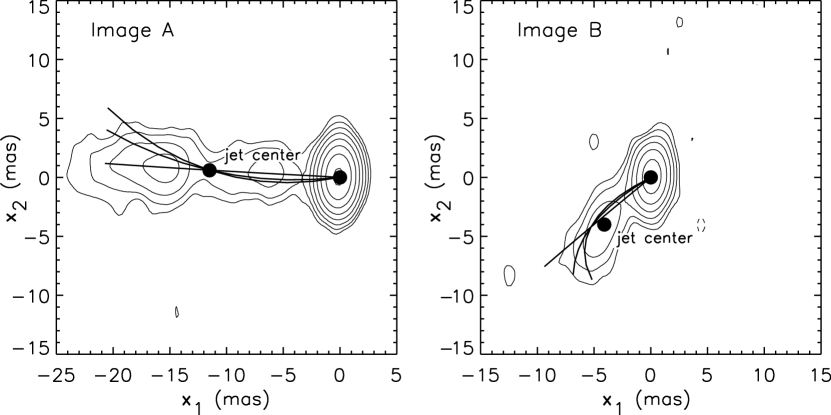
Figure 2: Models for the jet shape with no substructure. Using the best–fit smooth model the arc in image A is mapped onto the B image. The radio core is at the origin in both cases and the jet center is marked. The three arcs have curvatures of $|{\bf n_{A}}|=0$, 0.029 and 0.043 mas^-1 in image A and are designed to pass through both the core and the jet center. The model curves are overlayed on the Rusin et al. (2002) VLBI map. The lowest contour is 3 times the rms noise and each contour is increased by a factor of 2. The beam is $3.6\times 1.9$ with the larger axes being in the vertical $x_{2}$ direction.

A smooth model is fit to the positions of the lens galaxy, the radio cores of the images and the center of the jet images. A model is found that fits all the positions to better than 0.1 milli-arcsecond. In addition, the magnification ratio of the radio core agrees with the observed one to better than 10% despite this not being used as a constraint on the model. This signifies that the local magnification matrix, ${\bf\tilde{A}}$, is being accurately reproduced by the model. The velocity dispersion of the lens is $\sigma_{\rm host}=247\mbox{ km s${}^{-1}$}$ and the background shear is $\gamma=0.102$. This velocity dispersion is not unusual for a lens galaxy. The estimated circular velocity is $V_{\rm circ}=\sqrt{2}\sigma_{\rm host}$. The magnifications at the positions of the radio cores are $\mu_{A}=3.8$ and $\mu_{B}=-1.5$ – a negative magnification indicates a one dimensional parity flip in the image. This model gives a curvature magnification factor of $C=4.9$ at the center of the jet with image B being the more curved of the two images as observed. If the jet in image A has a curvature of $1/C$ times the curvature in image B and it is in the right direction then the observations can be explained without substructure. Figure 2 shows some attempts to model the jet in this way. From visual inspection it appears that the jet in image A is not bent enough to explain the bend in image B. The curve should follow the crest of the jet’s surface brightness, but a jet that is bent enough requires the end of the jet to be shifted by $\sim 3-4$ mas from the crest of the straight jet. The beam is large in this dimension, $3.6$ mas, but a shift in the crest should be detectable below this level.

Another way of evaluating this is to realize that

$$C\simeq\left(\frac{\theta^{A}_{\rm jet}}{\theta^{B}_{\rm jet}}\right)^{2}\frac{\delta^{B}}{\delta^{A}}$$ (15)

where $\theta_{\rm jet}$ is the length of the jet image and $\delta$ if the maximum deviation of the crest from a straight line. Judging from Rusin et al. (2002) $\theta^{B}_{\rm jet}\simeq 10\mbox{ mas}$, $\theta^{A}_{\rm jet}\simeq 22.0\mbox{ mas}$ and $\delta^{B}\simeq 2\mbox{ mas}$ giving $\delta^{A}\simeq 2\mbox{ mas}$ with the derived curvature magnification factor. This is small, but appears to be outside of the 12$\sigma$ contours along the full length of the jet in their map (the peaks in the jet are above 24$\sigma$). A more conclusive determination will probably require improved observations.

3.2.2 substructure

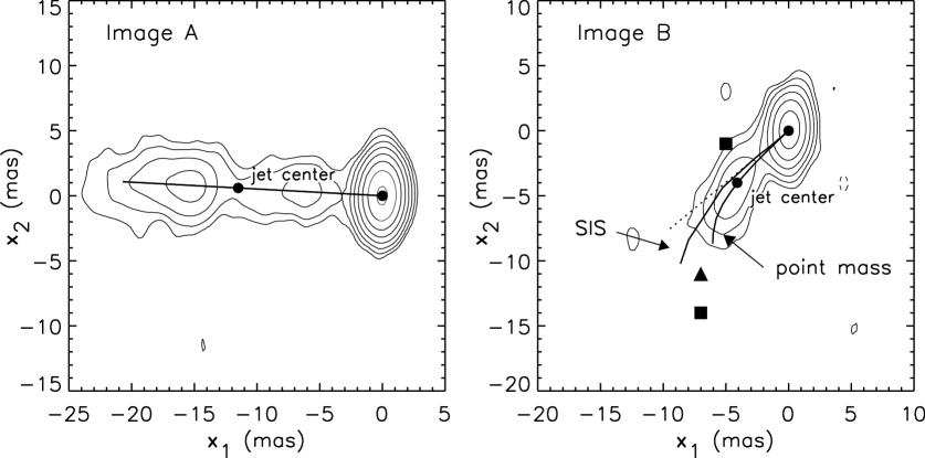
Figure 3: These are diagrams showing the reconstruction of Image B from a line segment representing Image A using the two lens models discussed in the text. The positions of the point mass substructure is marked by the triangle and the positions of the SIS substructures are marked by squares. The jets corresponding to each substructure model are marked with arrows. The dotted curve in the right hand panel is the image without any substructure. In the background is the Rusin et al. (2002) VLBI maps.

The substructure is modeled by adding either SIS or point masses to the smooth model described above. Several different methods for fitting the jet shape were tried. An essential difficulty is that besides the core there are no clear localized features along the jet that can be identified in both images. The positions of these features along with the tangent and curvature at such points could have been used as constraints were they present. Another difficulty arises from the large number of local minima in any $\chi^{2}$ function that was tried – there are different ways of bending a straight image by either “push” or “pulling” at different points.

It was found that the best and most unambiguous results were obtained by first fixing the smooth, or host, lens model to the one discussed in § 3.2.1. A straight line representing the jet in image A is then mapped to image B using the model. The substructures are added near image B by trial and error assisted by minimizing a $\chi^{2}$ based on the positions of the core and jet center until a curve in image B is obtained that best reproduces the qualitative features of the VLBI map. This method does not use the observed magnification ratio of the cores as a constraint so any possible contamination from microlensing by stars is entirely avoided. Figure 3 shows the results of this fitting. The resulting lens model is not unique in any quantitative sense, but there are clear things that can be learned from this fitting process about the kind of substructure that is capable of producing the bend.

When a point mass is used as a substructure the shape of image B is comparatively easy to reproduce. A point mass can be considered an approximation to any substructure that is very compact relative to its own Einstein radius such as a tidally truncated dark matter halo. Such a substructure can cause a strong deflection near its center while having a limited range of influence. This enables the point mass substructure in figure 3 to displace the lower end of the jet while leaving the position of the core end of the jet relatively unchanged. Note that the substructure has the effect of attracting the image rather than repelling it as would normally be the case. This attraction happens in only one dimension and is a result of one of the eigenvalues of the magnification matrix derived from the host lens being negative (image B is reflected in one dimension with respect to image A). The mass is most naturally calculated in units of the mass of the host lens within its Einstein radius which in this case is $M_{E}=(\sigma/c)^{4}G^{-1}\Sigma_{c}(z_{s},z_{l})^{-1}=1.6\times 10^{11}h_{65}^{-1}(\sigma/247\mbox{ km s${}^{-1}$})^{4}\mbox{ M}_{\odot}$. The favored model has a substructure mass of $m=2.5\times 10^{-5}M_{E}$. Other model parameters are summarized in table 1. A point mass with mass much more than $10^{-4}M_{E}$ tends to displace the lens without creating a bend and a mass of $\lower 2.15277pt\hbox{$\;\buildrel<\over{\sim}\;$}10^{-6}M_{E}$ cannot produce a bend on a large enough angular scale.

	Substructure Model Parameters
	$m/M_{E}$	$\sigma(\mbox{ km s${}^{-1}$})$	$x^{1}$ (mas)	$x^{2}$ (mas)	$\kappa$	$\mu_{\rm core}$
Point mass	$2.5\times 10^{-5}$	-	-7.0	-11.0	0.86	-1.19
SIS	-	9.6	-5.0	-1.0	1.05	-1.07
	-	21.0	-7.0	-14.0

Table 1: The positions $x^{1}$ and $x^{2}$ are the center of the substructure with respect to the core in image B. The surface density $\kappa$ and the magnification $\mu_{\rm core}$ are evaluated at the core in image B.

When a SIS model is used for the substructure it is difficult to reproduce the jet shape. The tendency is that when the SIS is massive enough to displace the lower end of the jet sufficiently it also displaces the core end of the jet so that a significant bend is not created – i.e. the SIS model is not compact enough. We partially get around this problem by using two SIS substructures in figure 3 and table 1, but even this does not produce very satisfactory results and considering the discussions in section 4 this seems an improbable explanation. It is possible that if the host lens model were allowed to vary along with the sublens model an explanation could be found that requires only one SIS substructure. However, including the host lens in the fitting process greatly increases the number of local minima in $\chi^{2}$ and after significant experimentation we have been unable to find a model that is a qualitative improvement on the one in figure 3 using a single SIS substructure. The two SIS model requires a precarious balance between the effects of two relatively massive substructures. A small change in the positions or masses causes the jet to be rather drastically distorted. We conclude that substructures as diffuse as SISs are an unlikely explanation for the observations.

By modeling the lens general conclusions can be made, but the specific form of the substructure is not tightly constrained. This modeling demonstrates that the bend in Q0957+561 can be reproduced by a sufficiently compact substructure. If the host lens model where changed to something other than a SIS+shear model substructure would still be needed if the jet is truly straight in image A and curved in image B. The new model would also need to reproduce the positions of the center of the jet relative to the core and the magnification ratio of the cores. Because of this the magnification matrix ${\bf\tilde{A}}$ could not be drastically different. The size, position and structure of the subclumps needed may change somewhat with the host model, but the general conclusions would still be the same.

4 Implications for Dark Matter and Cosmology

The structures responsible for the bend in image B of B1152+199 and the possible kink in image A of Q0957+561 are not terribly unusual in their mass or size. There are dwarf galaxies and globular clusters orbiting our galaxy that would fit the description. The importance lies in the likelihood of such a structure being close enough to the image to cause observable bending.

4.1 Estimated substructure densities

To estimate the probability of a jet like the one in B1152+199 having an observable bend, we will consider the bending effect of a single clump acting by itself. The host lens probably enhances the effect of the clump to a small degree. This will not change the results of this section by a large amount and so this extra complication will be neglected.

If we consider a straight line in the source plane that passes by a spherically symmetric lens centered at ${\bf x}_{0}$ with an impact parameter of $b$ the lensing equation (1) can be reduced to

$$b=\left[r\pm\alpha_{r}(r)\right]\cos(\theta)~{}~{}~{},~{}~{}~{}r>0$$ (16)

where $r\equiv|{\bf x}-{\bf x}_{0}|$, $\theta$ is the corresponding axial coordinate and $\alpha_{r}(r)$ is the radial deflection which is $<0$. The positive sign is used for $-\pi/2<\theta<\pi/2$ – the primary image – and the positive sign otherwise – the secondary image. We are concerned here only with the primary image; secondary images appear to form rarely in compound lensing with the mass scales considered here (Metcalf & Madau 2001) and they will generally be demagnified.

The curvature of the image can be calculated by taking derivatives of the curve (16). At the point $\theta=0$ the curvature is ${\bf n}(\theta=0)=\frac{1}{r^{2}}\left(\frac{d^{2}r}{d\theta^{2}}-r\right)\hat{\bf x}$. For our two models for the subclump this is

$${\bf n}(\theta=0)=\frac{-1}{\theta_{E}}\left\{\begin{array}[]{lc}\frac{1}{(x_{b}+\sqrt{x_{b}^{2}+4})^{2}}\left(\frac{3x_{b}^{2}+8}{\sqrt{x_{b}^{2}+4}}\right)~{}\hat{\bf x}&\mbox{(point mass)}\\ \frac{1}{(x_{b}+1)^{2}}~{}\hat{\bf x}&\mbox{(SIS)}\end{array}\right.$$ (17)

where $x_{b}\equiv b/\theta_{E}$. For the point mass $\theta_{E}=\sqrt{m/(\pi D_{l}^{2}\Sigma_{c})}$ and for the SIS $\theta_{E}=\lambda_{E}(\sigma)/D_{l}$.

A clump will not make an observable bend in a jet of length $\theta_{\rm jet}$ if the Einstein ring radius is either too big or too small. From (17) we see that the maximum curvature a clump can produce is $\theta_{E}(z)^{-1}$. When $\theta_{E}(z)$ is larger than the length of the jet the deviation from a straight line is at most $\sim\theta_{\rm jet}^{2}/8\theta_{E}$. This must be larger than the smallest measurable scale, $\theta_{\rm res}$, which is set by either the resolution of the observations or the width of the jet. Applying this criterion to the curvature as a function of $b$, (17), gives an upper limit on the impact parameter. A small clump will influence a region of the jet of size $\sim\theta_{E}$. If the smallest scale $\theta_{\rm res}$ is of order the circumference of the Einstein ring then its bending effects will be on too small a scale to be observed. These constraints are summarized as

$$\frac{\theta_{\rm res}}{2\pi}\lower 2.15277pt\hbox{$\;\buildrel<\over{\sim}\;$}\theta_{E}\lower 2.15277pt\hbox{$\;\buildrel<\over{\sim}\;$}\frac{\theta^{2}_{\rm jet}}{8\theta_{\rm res}}~{}~{}~{}~{},~{}~{}~{}~{}|{\bf n}(x_{b})|\lower 2.15277pt\hbox{$\;\buildrel>\over{\sim}\;$}\frac{8\theta_{\rm res}}{\theta^{2}_{\rm jet}}$$ (18)

The first of these inequalities can be used to find the range of velocity dispersions or masses that could be responsible an observable bending of the jet in B1152+199:

$$6\mbox{ km s${}^{-1}$}\lower 2.15277pt\hbox{$\;\buildrel<\over{\sim}\;$}\sigma\lower 2.15277pt\hbox{$\;\buildrel<\over{\sim}\;$}13\mbox{ km s${}^{-1}$}$$ (19)

$$7.1\times 10^{4}h_{65}^{-1}\mbox{ M}_{\odot}\lower 2.15277pt\hbox{$\;\buildrel<\over{\sim}\;$}m\lower 2.15277pt\hbox{$\;\buildrel<\over{\sim}\;$}2.7\times 10^{7}h_{65}^{-1}\mbox{ M}_{\odot}$$ (20)

where the values $\theta_{\rm jet}=15$ milli-arcsec and $\theta_{\rm res}=3$ milli-arcsec have been used. This range is consistent with the $\sigma$ derived in § 3.2. The true ranges are probably a bit larger because of the influence of the host lens which will increase the sensitive to smaller mass objects. The second of the inequalities (18) puts an upper limit on the impact parameter $b$ as a function of $\sigma$ or $m$ through (17). By plugging in the smallest allowed clump we can find the largest possible impact parameter – $b\lower 2.15277pt\hbox{$\;\buildrel<\over{\sim}\;$}1.6\,{\rm mas}=10h_{65}^{-1}$ pc for the SIS and $6.9\,{\rm mas}=28h_{65}^{-1}$ pc for the point mass. The clump needs to be quite well aligned with the image.

The probability of a subclump bending the jet will be taken to be $p\propto\theta_{\rm jet}db$ within the allowed range of $b$. The probability or expected number of important clumps per jet is

$$p\simeq 2\theta_{\rm jet}\frac{c}{H_{0}}\int_{0}^{z_{s}}\frac{dz}{(1+z)}\frac{D(z)^{2}}{E(z)}\int^{m_{\rm max}(z)}_{m_{\rm min}(z)}dm~{}b_{\rm max}(m,z)\frac{d{\mathcal{N}}}{dm}(m,z)$$ (21)

where ${\mathcal{N}}$ is the 3–dimensional number density of clumps and $E(z)=\left[\Omega_{m}(1+z)^{3}+\Omega_{R}(1+z)^{2}+\Omega_{\Lambda}\right]^{1/2}$, $\Omega_{R}=1-\Omega_{m}-\Omega_{\Lambda}$. In the case of SIS lenses $m$ can be replaced with $\sigma$ and $b_{\rm max}(\sigma,z)$ can be found explicitly. For the point mass case $b_{\rm max}(m)$ must be found numerically.

To get a simple estimate of the number density of clumps required we can take them to all lie within the host lens and give them all the same velocity dispersion. In this case (21) reduces to

$$p\simeq 2\theta_{\rm jet}^{2}D_{l}^{2}\,\eta(\sigma)\left(\sqrt{\frac{2\theta_{E}(\sigma)}{\theta_{\rm res}}}-\frac{\theta_{E}(\sigma)}{\theta_{\rm jet}}\right)~{}~{}~{}~{}~{}~{}\mbox{(SIS)}$$ (22)

where $\eta(\sigma)$ is the 2–dimensional number density of clumps. The range of allowed $\sigma$ given in (19) gives a range $\eta(\sigma)/p\simeq 32-111~{}h_{65}^{2}\mbox{ kpc}^{-2}$. This is the number density of substructures required to make the bending commonplace. The same exercise with point masses in the range $m=10^{5}-10^{7}\mbox{ M}_{\odot}$ gives a range of $\eta(\sigma)/p\simeq 130-260~{}h_{65}^{2}\mbox{ kpc}^{-2}$ or $\Sigma=1.3\times 10^{7}-2.6\times 10^{9}\mbox{ M}_{\odot}\mbox{ kpc}^{-2}$ where the higher mass density is for larger mass clumps. In units of the critical density this is $\kappa=0.005-0.99$. This value is anywhere from a few percent to more than all of the surface density of the host lens. The lensing effect of the host lens may reduce these estimates by a factor of roughly $|\mu|^{-1/2}$ – an estimate of the eigenvalues of the magnification matrix – which is 0.3–0.9 for the model found in § 3.2.

Instead of fixing the mass of the substructure we can guess at a realistic mass function. One expects that the number density of small mass clumps will be proportional to the density of all matter, $\rho$, averaged over a larger scale than the clumps being considered – constant Lagrangian number density. CDM simulations and analytic estimates predict a power–law mass function for the low mass range important here,

$$\frac{1}{\rho}\frac{d{\mathcal{N}}}{dm}=\frac{1}{M_{o}m_{o}}\left(\frac{m}{m_{o}}\right)^{\alpha}$$ (23)

where $m_{o}$ and $M_{o}$ are normalization constants. Fitting the mass function from $\Lambda$CDM N–body simulations to the observed velocity distribution in the range $V_{\rm circ}=20-400\mbox{ km s${}^{-1}$}$ gives the relation $\sigma\simeq 100\mbox{ km s${}^{-1}$}(m/3.0\times 10^{11}\mbox{ M}_{\odot})^{1/3}$. For SIS substructures this relation is used to convert (23) into a distribution of velocity dispersions where it is extrapolate below $V_{\rm circ}=20\mbox{ km s${}^{-1}$}$. In $\Lambda$CDM simulations the dark matter clumps have $\alpha\simeq-1.91$ and $M_{o}=4.8\times 10^{12}h^{-1}\mbox{ M}_{\odot}$ for $m_{o}=3.0\times 10^{11}\mbox{ M}_{\odot}$ (Klypin et al. 1999). The exponent for the $\sigma$ distribution is $\alpha_{\sigma}=-3.73$ in this case. This distribution fits the observed distribution of dwarf galaxies near $\sigma=50-100\mbox{ km s${}^{-1}$}$ above which the contribution to (21) is small.

Using the full range of masses in (19) and keeping all the subclumps at the redshift of the host lens results in a probability of $p\simeq 3.2\,\kappa$ where $\kappa$ is the surface density of the host lens, $\kappa=0.35$ and $0.85$ for the model in § 3.2. Figure 4 shows $p$ and the fraction of the halo mass density contained in substructure as a function of a lower mass cutoff in the mass function. The smaller mass clumps contribute most of the probability, but little of the mass density. This mass fraction is a lower limit in that if the internal structure of the subclumps is less centrally concentrated it will require more mass to reach the same probability. For SIS substructures that are not tidally truncated $p=1.9\times 10^{-3}\,\kappa$. To increase this probability by a factor of ten would require the entire mass density of the host lens to be composed of SISs in the range (19). Any tidal truncation will reduce SIS substructures’ lensing effect.

Objects that are not in the host galaxy, but happen to lie near the line of sight could also cause bending of the jet. To estimate this contribution we integrate (21) with the mass function (23) assuming that $\rho$ along the line of sight is given by the average density of the universe. For SIS structure $p=1.3\times 10^{-4}$ and for point masses with the same mass function $p=0.65$. This extra–galactic population is only an important contribution to the probability if the clumps are very compact in which case it is comparable to the contribution from substructures inside the lens.

The CDM model does seem capable of accounting for the bent jets, provided DM halos are relatively compact. If the radius is small compared to the Einstein radius of a point mass of the same mass ($r\lower 2.15277pt\hbox{$\;\buildrel<\over{\sim}\;$}\theta_{E}=11(m/10^{6}\mbox{ M}_{\odot})^{1/2}h_{65}^{1/2}\mbox{ pc}$) less than $\sim 10\%$ of the mass need be in substructure. However, any less concentrated clumps will require more total mass. The SISs require much more mass. The Navarro, Frenk & White (NFW) profile (Navarro, Frenk, & White 1997), $\rho(r)=\rho_{c}r_{s}^{3}r^{-1}(r_{s}+r)^{-2}$, is believed to be more realistic for pure dark matter halos. If $r_{s}$ is small compared to the above limit and a large fraction of the mass is within this radius then the mass fraction might get down to the levels shown in figure 4. The scale length according to the standard structure formation scenario is $r_{s}=2.17\times 10^{3}{\rm c}^{-1}h_{65}^{-2/3}(m_{200}/10^{6}\mbox{ M}_{\odot})^{1/3}\mbox{ pc}$ where c is the concentration and $m_{200}$ is the virial mass. If the concentration is 100 or larger then the core is compact enough, but in this case the mass within $r_{s}$ is less than 10% of $m_{200}$. In addition, $c\simeq 100$ is a bit high for a straightforward extrapolation of the simulations (Bullock et al. 2001) – no simulation has been done with a resolution high enough to resolve these mass scales. To achieve the same probability for bending the jet, it seems that any realistic CDM model will require significantly more mass – at least before tidal stripping occurs – to be in small scale structure than is required in the point mass model used here.

Also, the survival of substructure in the host lens is a complicated issue. Clumps with $m\lower 2.15277pt\hbox{$\;\buildrel>\over{\sim}\;$}10^{7}\mbox{ M}_{\odot}$ are not likely to survive within the inner few kpc because they lose orbital energy to dynamical friction and fall into the center of the galaxy where they are destroyed by tides. This upper mass cutoff can significantly change the local fraction of mass in substructures while not affecting the lensing probability greatly.

4.2 Contribution from known structures

There are about 40 known dwarf galaxies in the Local Group (Mateo 1998; Klypin et al. 1999). Most of these are within $\sim 300\mbox{ kpc}$ of either the MW or M31. About twenty eight of these have circular velocities above $10\mbox{ km s${}^{-1}$}$. This gives an estimated surface number density of $\sim 3.5\times 10^{-5}\mbox{ kpc}^{-2}$ if they were uniformly distributed in this volume. There are about 200 globular clusters in the MW with masses of $10^{4}-10^{6}\mbox{ M}_{\odot}$ making their number density an order of magnitude larger. The concentration of dwarfs and globular clusters toward the center of the galaxy and observational incompleteness might increase this estimate by a factor of several, but nowhere near enough to reach the required number densities derived in the previous section.

Another way of estimating the contribution from dwarf galaxies is to use the mass function (23) converted to velocity dispersion. For the observed galaxies within $200h^{-1}$ kpc of the MW and M31 $\alpha_{\sigma}=-2.35\pm 0.4$ and $m_{o}\simeq M(<200)/6.32$ for $\sigma_{o}=10\mbox{ km s${}^{-1}$}$ where $M(<200)$ is the total mass within $200h^{-1}$ kpc (Klypin et al. 1999). We will use $M(<200)=10^{12}\mbox{ M}_{\odot}$. With SIS dwarf galaxies this velocity distribution gives a probability for bending the jet of $p=3.9\times 10^{-6}\,\kappa$ if the dwarfs are in the host lens. Figure 4 shows $p$ as a function of a lower $\sigma$ cutoff which is converted into mass by $\sigma=100\mbox{ km s${}^{-1}$}(m/3.0\times 10^{11}\mbox{ M}_{\odot})^{1/3}$. If the same velocity distribution is used for the entire line of sight at the average mass density, $p=2.7\times 10^{-7}$. Dwarf galaxies are not compact enough to be considered point mass lenses, but by treating them as point masses we can get an (probably greatly inflated) upper limit on the probability. In this case $p=8.9\times 10^{-5}\,\kappa$.

Known types of substructure within the host lens are inadequate to explain B1152+199. If the structures in the lens and in intergalactic space are similar in number and central density to those observed in the local group of galaxies they fall short of the estimates derived in § 4.1 by at least a factor of $10^{5}$.

Figure 4: The probability of substructures causing an observable bend in a radio jet like the one in B1152+199 assuming the distribution of substructures described in the text. For the SIS substructures the velocity dispersion is converted to mass by $m=3.0\times 10^{11}\mbox{ M}_{\odot}(\sigma/100\mbox{ km s${}^{-1}$})^{3}$. The fraction of the host halo surface density contained in point mass substructure is also plotted. The host lens surface density is $\kappa=0.6-1.4$ for the model of B1152+199 discussed in § 3.2.

5 Discussion

These observations have important consequences for the Warm Dark Matter (WDM) model. The standard WDM model is engineered to reproduces the dwarf galaxy distribution under the assumption that a galaxy forms in every small halo. It was shown in § 4.2 that the number density of dwarf galaxies is extremely unlikely to have produced the observed bent radio jets. The standard WDM model is thus ruled out if the bend in B1152+199 is real. A more accurate lower limit on the DM particle mass will require more observations and more simulations of small scale structure formation in these models.

Higher resolution observations of B1152+199 are possible. These would make certain that the jet in image B is indeed bent and improve the constraints on the substructure mass. Also interesting would be high resolution images of other multiply imaged jets. In the present sample of three all appear to show some evidence of bending. A moderately larger sample would greatly increase the power of this method to probe structure on small scales.

It has been found here that a significantly larger number of small scale objects are needed if the observations of B1152+199 are to be simply interpreted. Structures as diffuse as SIS are disfavored both by direct modeling of B1152+199 and on statistical grounds. If the structures are compact (on the scale of their own Einstein radius) and small in mass ($\lower 2.15277pt\hbox{$\;\buildrel<\over{\sim}\;$}10^{7}\mbox{ M}_{\odot}$) they need not contain a large fraction of the mass in the universe. However, such concentrated halos come about in the CDM model only through the tidal stripping of halos that originally contained $\sim 10$ times more mass. This means that in intergalactic space these clumps would contain a large fraction of the mass, perhaps most of it.