Effect of a wide binary companion to the lens
on the astrometric behavior of gravitational microlensing events

Abstract

In this paper, we investigate the effect of a wide binary companion of the lens on the astrometric behavior of Galactic gravitational microlensing events and compare it to the effect on the photometric behavior. We find that the wide binary companion of the lens can affect the centroid motion of images substantially even if the corresponding light curve appears to be the one of a standard single point-mass lens event. The relatively significant effect of the wide binary lens on the astrometric lensing behavior, on one side, calls for careful consideration of the lens binarity in analyzing the future astrometric lensing data. On the other side, larger astrometric effect of the companion makes astrometric lensing an efficient method to detect binary lenses over a broad range of separations.

1 Introduction

Light curves of microlensing events caused by a single point-mass lens are characterized by non-repeating, single peak, and symmetric curves (Paczyński, 1986), known as Paczyński curves. On the other hand, if events are caused by a binary lens, the resulting light curves deviate from those of single lens events. The deviation caused by the binary nature of the lens becomes prominent when the angular separation between the two lens components (binary separation) is comparable to the angular Einstein ring radius of the lens system, which is related to the physical parameters of the system by

$$\theta_{\rm E} = \left(\frac{2R_{\rm Sch}}{D}\right)^{1/2}$$ (1)

$$\sim 0.72\ \mbox{mas}\left(\frac{D_{\rm S}}{D_{\rm L}}-1\right)^{1/2}\left(\frac{D_{\rm S}}{8\ \mbox{kpc}}\right)^{-1/2}\left(\frac{M}{0.5\ \mbox{M${}_{\sun}$}}\right)^{1/2}$$

where $D^{-1}=D_{\rm L}^{-1}-D_{\rm S}^{-1}$, $D_{\rm L}$ and $D_{\rm S}$ are the distances to the lens and the source from the observer respectively, and $R_{\rm Sch}$ is the Schwarzschild radius corresponding to the total mass $M$ of the lens system. As the binary separation becomes larger, however, the individual lens components begin to act as if they are two independent single lenses. For these wide binary lens systems, it is likely that the source trajectory will pass close only to one of the lens components and the resulting light curve will look very similar to a standard Paczyński curve. If the Galactic binaries have a similar distribution of binary separations to that of binaries in the solar neighborhood (Duquennoy & Mayor, 1991), the majority of the binaries located along the lines of sight towards the Galactic bulge will have separations substantially larger than their Einstein ring radii whose typical values are several hundred micro- to a few milli-arcseconds. Therefore, for most of Galactic binary lens events, it will be difficult to identify the existence of the companion to the lens from the analysis of the light curves alone except for the rare case of either caustic crossing or the source star’s passage near both lens components (a repeating event; Di Stefano & Scalzo, 1999).

As an alternative method of microlensing observations, it was proposed to measure the lensing-induced displacement of the (brightness-weighted) image centroid position (usually referred to centroid shifts) by high precision astrometry (Miyamoto & Yoshii, 1995; Høg, Novikov, & Polanarev, 1995; Walker, 1995; Miralda-Escudé, 1996; Paczyński, 1998; Boden, Shao, & Van Buren, 1998; Han & Chang, 1999; Dominik & Sahu, 2000). When a source star is microlensed, it becomes split into several images whose number depends on the structure of the lens system, e.g., two images for a single lens and three or five images for a binary lens system. The typical separation between the images is an order of $\theta_{\rm E}$, and thus it is impossible to resolve the individual images even with the highest angular resolution achieved so far. However, several planned high-precision astrometric satellite experiments, e.g., Space Interferometry Mission (SIM), Double Interferometer for Visual Astrometry (DIVA), and Global Astrometric Interferometer for Astrophysics (GAIA), and optical/NIR interferometers on 10-m class ground-based telescopes, e.g., the Keck interferometer, the Very Large Telescope Interferometer (VLTI), and the Large Binocular Telescope (LBT), will have precisions in position measurements of the order of tens of $\mu$-arcsecs or better, and thus will enable one to measure the lensing-induced centroid shifts.

If an event is caused by a point-mass lens, the trajectory of the centroid shifts traces an ellipse (see § 2), known as an astrometric ellipse (Walker, 1995; Jeong, Han, & Park, 1999; Dominik & Sahu, 2000). If an event is caused by a binary lens, on the other hand, the centroid shift trajectory deviates from the elliptical one of a single lens event, which is characterized by distortions, twistings, and jumps (Han, Chun, & Chang, 1999).

In this paper, we investigate how a wide binary companion of the lens affects the observed photometric and astrometric microlensing behaviors. From this investigation, we find that the effect on the trajectory of the image centroid shifts is significantly more important than on the light curve. Hence, we argue that a careful consideration of the effect of a wide binary lens will be required in analyzing the measured centroid shifts even if the corresponding light curve appears to be a standard Paczyński curve.

2 Basics of Microlensing

If a source located at $\mbox{\boldmath$r$}_{\rm S}$ (on the projected plane of the sky) is lensed by a $N$-point-mass lens system, where the individual components’ masses and locations are $m_{i}$ and $\mbox{\boldmath$r$}_{{\rm L},i}$, the positions of the images $r$ are obtained by solving the equation of lens mapping (the lens equation);

$$\mbox{\boldmath$r$}_{\rm S}=\mbox{\boldmath$r$}-\theta_{\rm E}^{2}\sum_{i=1}^{N}\frac{m_{i}}{M}\frac{\mbox{\boldmath$r$}-\mbox{\boldmath$r$}_{{\rm L},i}}{|\mbox{\boldmath$r$}-\mbox{\boldmath$r$}_{{\rm L},i}|^{2}}\,,$$ (2)

where $M=\sum_{i}^{N}m_{i}$. Since the lensing process conserves the surface brightness (i.e. does not create nor destroy photons), the flux ratio between the lensed image and the unlensed source is simply given by the surface area ratio between the image and the unmagnified source, i.e., the magnification. For a point source limit, the magnifications of the individual images are given by the inverse of the Jacobian determinant of the lens mapping evaluated at each image position $\mbox{\boldmath$r$}_{j}$;

$$A_{j}=\left(\frac{1}{|\det J|}\right)_{\mbox{\boldmath$r$}=\mbox{\boldmath$r$}_{j}}\ ;\ \ \ \det J=\left|\frac{\partial\mbox{\boldmath$r$}_{\rm S}}{\partial\mbox{\boldmath$r$}}\right|\,$$ (3)

and the total magnification is given by the sum of the magnifications of the individual images, i.e., $A_{\rm tot}=\sum_{j}^{N_{\rm I}}A_{j}$, where $N_{\rm I}$ is the total number of images. The location of the apparent image centroid corresponds to the magnification weighted mean of the individual image positions, and therefore, the centroid shift is given by

$$\mbox{\boldmath$\delta$}=\sum_{j}^{N_{\rm I}}\frac{A_{j}}{A_{\rm tot}}\mbox{\boldmath$r$}_{j}-\mbox{\boldmath$r$}_{\rm S}\ .$$ (4)

For a single point-mass lens ($N=1$), the lens equation (eq. [2]) is easily solvable and solving the equation yields two image positions ($N_{\rm I}=2$). The total magnification and the centroid shift of the single lens event are expressed in analytical forms of

$$A=\frac{u^{2}+2}{u\sqrt{u^{2}+4}}\,;$$ (5)

$$\mbox{\boldmath$\delta$}=\frac{\theta_{\rm E}\mbox{\boldmath$u$}}{u^{2}+2}\,,$$ (6)

where $\mbox{\boldmath$u$}\equiv(\mbox{\boldmath$r$}_{\rm S}-\mbox{\boldmath$r$}_{\rm L})/\theta_{\rm E}$ is the dimensionless lens-source separation vector normalized by $\theta_{\rm E}$. Since the source and the lens move relative to each other, $u$ changes with time. Under the approximation that this relative motion is rectilinear, it is represented by

$$\mbox{\boldmath$u$}=\left(\frac{t-t_{0}}{t_{\rm E}}\right)\hat{\mbox{\boldmath$x$}}+\beta\hat{\mbox{\boldmath$y$}}\,,$$ (7)

where $t_{\rm E}$ represents the time required for the source to transit $\theta_{\rm E}$ (Einstein time scale), $\beta$ is the closest lens-source separation in units of $\theta_{\rm E}$ (impact parameter), $t_{0}$ is the time at that moment, and the unit vectors $\hat{\mbox{\boldmath$x$}}$ and $\hat{\mbox{\boldmath$y$}}$ are parallel and perpendicular to the direction of the relative lens-source motion, respectively. The trajectory of the centroid shifts is an ellipse with a major axis and an eccentricity of $a=(\theta_{\rm E}/2)\times(\beta^{2}+2)^{-1/2}$ and $e=[(\beta^{2}/2)+1]^{-1/2}$ and its semi-major axis lies parallel to $\hat{\mbox{\boldmath$x$}}$.

For a multi-lens system ($N\geq 2$), on the other hand, the lens equation cannot be solved algebraically. Hence, to obtain the image positions, one has to solve the equation numerically. In particular, for the case of a binary lens ($N=2$), the lens equation can be expressed as a fifth-order complex polynomial (Witt, 1990) and there exist three or five images depending on the source position with respect to the lens positions.

3 Effects of a Wide Binary Lens Companion

The existence of a binary companion to the lens affects both the photometric and astrometric behaviors of a microlensing event. The most important effect of a wide binary companion of the lens is that it makes the effective position of the primary move towards it or, equivalently, the effective source position move with respect to the primary (Di Stefano & Mao, 1996). From the lowest order approximation of equation (2), one finds that this effect is well characterized by the use of an effective lens-source separation vector, which is expressed by

$$\tilde{\mbox{\boldmath$u$}}\equiv\mbox{\boldmath$u$}_{1}-\frac{q}{d}\frac{\mbox{\boldmath$r$}_{{\rm L},2}-\mbox{\boldmath$r$}_{{\rm L},1}}{|\mbox{\boldmath$r$}_{{\rm L},2}-\mbox{\boldmath$r$}_{{\rm L},1}|}\,,$$ (8)

where the subscripts ‘1’ and ‘2’ represent the primary and the companion respectively, $q=m_{2}/m_{1}$ is the mass ratio, and $\mbox{\boldmath$u$}_{1}=(\mbox{\boldmath$r$}_{\rm S}-\mbox{\boldmath$r$}_{{\rm L},1})/\theta_{{\rm E},1}$, and $d=|\mbox{\boldmath$r$}_{{\rm L},2}-\mbox{\boldmath$r$}_{{\rm L},1}|/\theta_{{\rm E},1}$ are the distances of the source and the companion from the primary lens normalized by the Einstein ring radius of the primary $\theta_{{\rm E},1}$, respectively. We note that this effect is not generally measurable because it requires an a priori information on the actual positions of the lens components on the sky.

As an additional effect of the binary lens companion, one may expect that the observed light curve and the centroid shift trajectory would be the superposition of those resulting from the two events in which the component lenses behave as two independent lenses. However, this superposition effect of the lens companion is important only for the trajectory of the centroid shifts but not for the light curve of an event. This can be seen from the magnification and the centroid shift caused by the companion when the source is located close to the primary (i.e., $\mbox{\boldmath$r$}_{\rm S}\simeq\mbox{\boldmath$r$}_{{\rm L},1}$), which are, respectively, represented by

$$A_{2}\sim 1+2\frac{q^{2}}{d^{4}}\ \ \ ({\rm for}\ d\gg 2)\,,$$ (9)

$$\delta_{2}\sim\theta_{{\rm E},1}\frac{q}{d}\ \ \ ({\rm for}\ d\gg\sqrt{2})\ .$$ (10)

From equations (9), one finds that as the binary separation becomes larger, the photometric superposition effect falls off rapidly ($\sim d^{-4}$): faster than the decrease of $|\tilde{\mbox{\boldmath$u$}}-\mbox{\boldmath$u$}_{1}|$ ($\sim d^{-1}$; see eq. [8]). On the other hand, the astrometric effect endures up to a very large separation at which the photometric effect is negligible (the same order effect as the positional shift; see eq. [10]).

To illustrate the larger astrometric superposition effect of the lens companion than its photometric effect, we present the light curves (Fig. 1) and the trajectories of the image centroid shifts (Fig. 2) of events caused by a wide binary lens with the mass ratio $q=0.3$ and the separation $d=5.7$. One finds that the light curves of these events are well approximated by that of a single lens event after accounting for the effective positional shift of the primary. By contrast, the corresponding centroid shift trajectories deviate significantly from an elliptical one expected for a single lens event.

4 Detection of Wide Binary Lens Companions

In order to assess how well one can distinguish light curves of wide binary lensing events from the ones of single point-mass events, we define an magnification excess by

$$\epsilon=\frac{A-\tilde{A}_{0}}{\tilde{A}_{0}}\,,$$ (11)

where $A$ is the exact magnification of the wide binary lens event and $\tilde{A}_{0}$ is that of the single lens event with a mass equal to the primary and located at the effective position defined by equation (8),

$$\tilde{A}_{0}=\frac{\tilde{u}^{2}+2}{\tilde{u}\sqrt{\tilde{u}^{2}+4}}\ .$$ (12)

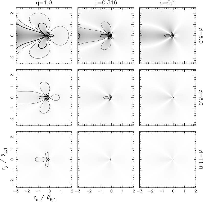
Figure 3: Contour maps of magnifications excess, $\epsilon$ (see eq. [11] for the definition). The binary separations and the mass ratios of the binary lenses shown are $q=1.0,\ 0.316,\ 0.1$ and $d=5.0,\ 8.0,\ 11.0$. All scales are normalized by the Einstein ring radius of the primary, $\theta_{{\rm E},1}$. The origin is the position of the primary and the companion is located on the left side of the primary, i.e. ($-d$, 0). Contours are drawn at the levels of $\epsilon=\pm$3% (thick lines) and $\pm$1% (thin lines). In addition to the contours, grey scale is used to provide the idea of the gradient over the region.

Figure 3 shows the magnification excess map of the region close to the primary lens for wide binary lens systems with various values of $d$ and $q$. From the figure, one finds that the region of significant deviations shrinks rapidly as $d$ increases. Noticeable deviations (e.g., $\epsilon\gtrsim 2$%) occur only if the source passes very close to the primary, implying that the presence of the companion to the lens can be detected effectively only if the source crosses the caustic associated with the primary or passes the region of the cusp-influence magnification. However, both the size of the caustic and the strength of the cusp converge to those of a point-mass lens much faster than the effect of the positional shift. As a result, even with the photometric precision as good as 0.01 mag and sufficiently dense sampling during the peak magnification, the binary detection efficiency is expected to be low for most wide binary microlensing events with $d\gtrsim 10$.

In order to compare the photometric deviation to the one expected from astrometric observations, we also define the deviation of centroid shift by

$$\Delta\mbox{\boldmath$\delta$}=\mbox{\boldmath$\delta$}-\tilde{\mbox{\boldmath$\delta$}}_{0}\,,$$ (13)

where $\delta$ is the centroid shift of the wide binary lensing event while $\tilde{\mbox{\boldmath$\delta$}}_{0}$ represents the centroid shift caused by the primary alone placed at its effective position,

$$\tilde{\mbox{\boldmath$\delta$}}_{0}=\frac{\theta_{{\rm E},1}\tilde{\mbox{\boldmath$u$}}}{\tilde{u}^{2}+2}\ .$$ (14)

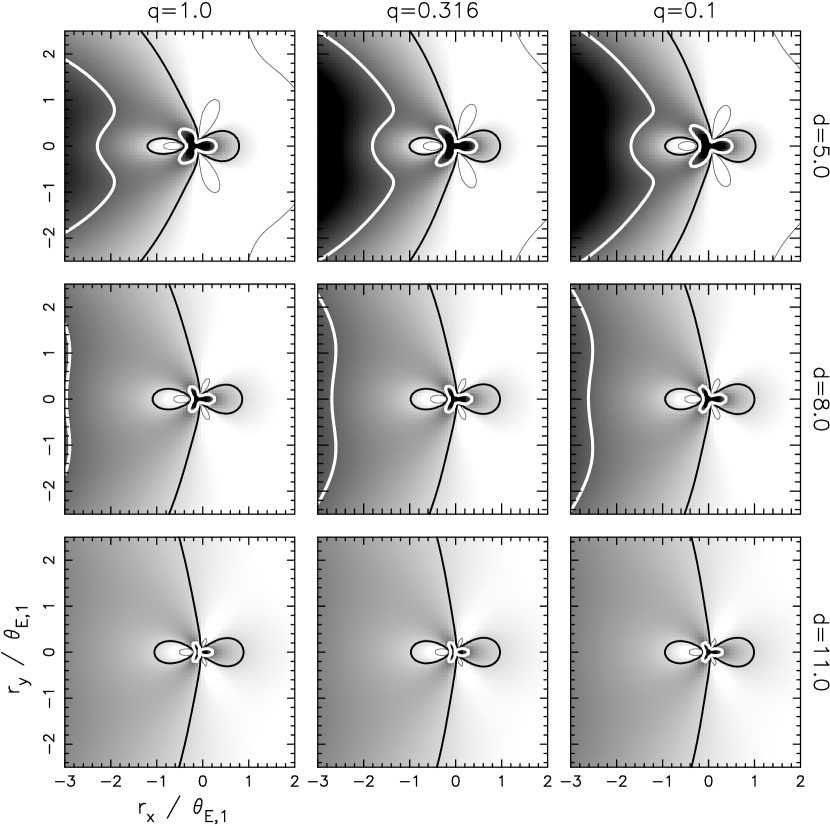
Figure 4: Contours of centroid shift deviations, $\Delta\delta$ (see eq. [13]), in the same region and for the same wide binaries as in Fig. 3. The coordinate systems are also the same as in Fig. 3. Contours are drawn at the levels of $\Delta\delta=(2/3)\times(q/d)\times\theta_{{\rm E},1}$ (thin black lines), $q/d\times\theta_{{\rm E},1}$ (thick black lines), and $(3/2)\times(q/d)\times\theta_{{\rm E},1}$ (thicker white lines). Grey scale is used to provide the idea of the gradient over the region, but does not necessarily correspond to the absolute values of deviations.

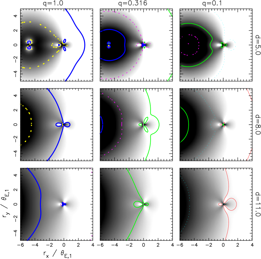
Figure 5: Contours of centroid shift deviations, $\Delta\delta$ (see eq. [13]), for the same wide binaries as in Figs. 3 and 4 but in the wider region around primary. The coordinate systems are the same as in Figs. 3 and 4. Contours are drawn at the levels of $\log(\Delta\delta/\theta_{{\rm E},1})=-2.1,\ -1.8,\ -1.5,\ -1.2,\ -0.9,\ -0.6$ with colors of Red, Cyan, Green, Magenta, Blue, Yellow. Grey scale is used to provide the idea of the gradient over the region, but does not necessarily correspond to the absolute values of deviations.

Figure 4 shows the contour maps of $\Delta\delta$ of the same region and for the same binaries as in Figure 3. When the source is located near the primary, the centroid shift deviation – mostly due to the superposition effect – is an order of $\sim(q/d)\theta_{\rm E,1}$ (see eq. [10]). Therefore, we draw contours at the levels which are scaled by $(q/d)\theta_{\rm E,1}$. Figure 5 show the maps in a wider region where the contours are drawn at 6 different levels ranging $\sim 1\%$ to $\sim 25\%$ of $\theta_{{\rm E},1}$. Considering that the size of the angular Einstein ring radius is an order of a few milli- to several hundred micro-arcseconds for events caused by Galactic G, K, and M dwarfs with masses in the range of $\sim 0.1\ \mbox{M${}_{\sun}$}$ – $1\ \mbox{M${}_{\sun}$}$ (see eq. [1]), the deviations for the events caused by a binary lens even with $q/d\sim 0.01$ are expected to be still several micro-arcseconds, which is comparable to the expected astrometric precision of the new generation interferometers. Moreover, large deviations are found throughout the map, rather than concentrating near the primary as in the map of magnification excess. Notably, quite complex patterns of deviation are present over the region of the circle around the primary with the radius of about $\theta_{\rm E,1}$ even for the case of $d\sim 10$. This implies that the astrometric deviation will typically last for $\sim t_{\rm E}$. From astrometric microlensing observations of events, therefore, one can detect the presence of binary companions to the lens for a broader range of separations with an increased efficiency than from conventional photometric observations, possibly even with less dense sampling.

As a quantitative comparison between the detection efficiencies of wide binary companions to the lens expected from the photometric and the astrometric lensing observations, we perform a Monte-Carlo simulation. In the simulation, we produce a large number of wide binary lens events and fit their light curves and image centroid shift trajectories to those of single point-mass lens events (eqs. [5] and [6]). We assume the lens binarity is detected if the resulting $\chi^{2}$ of the fit is larger than a statistically acceptable value (see below). Tables 1 and 2 list the photometric and astrometric detection rate determined by the simulation, each for the same wide binaries as Figures 3 and 4 under two different sampling strategies and three different measurement errors. The resulting detection rate in each entry is based on 5,000 trial simulations. We note that, since we are more interested in the possibility of the inference to the presence of the lens companion, rather than in the determination of the absolute detection efficiency, we exclude the repeating events and the caustic-crossing events for which the binarity of the lens can be immediately inferred. Trial events are generated with random trajectories for each fixed configuration of the binary (i.e, at fixed $d$ and $q$), but restricted only to high-magnification, non-repeating, and non-caustic-crossing events. To simulate light curves, we fix the unlensed source flux at an arbitrary value and include also random amounts of blended light of less than 20% of the unlensed source flux. As for the observation, we examine two different types of sampling. In the first type, we assume 200 photometric and astrometric measurements during $-t_{\rm E}\leq t_{\rm obs}-t_{0}\leq 3t_{\rm E}$ (‘Broad’ sampling). In the second type, the same number of measurements are performed during a shorter period of time around the photometric peak of $-0.5t_{\rm E}\leq t_{\rm obs}-t_{0}\leq 1.5t_{\rm E}$ (‘Dense’ sampling). For simplicity, the sampling rate is taken to be uniform and the uncertainty associated with each measurement is the same throughout the measurements (i.e., the deviations distribute as Gaussian with a single variance). Finally, the best-fitting single lens model and $\chi^{2}$ of a simulated event are determined through the $\chi^{2}$ minimization by successive linearized fitting. For light curves, we fit five parameters: $t_{0}$, $t_{\rm E}$, $\beta$, and the unlensed source flux and the blended light while, for the image motion, we fit seven parameters: $t_{0}$, $t_{\rm E}$, $\beta$, $\theta_{\rm E}$, and the direction of the relative lens-source motion and the lens position on the sky (which is characterized by two parameters). The detection is defined by

$$\sqrt{2\chi^{2}}-\sqrt{(2\cdot{\rm dof}-1)}\geq 3\,,$$ (15)

where ‘${\rm dof}$’ denotes the degrees of freedom of the fitting. The criterion was chosen to be the 3$\sigma$ deviation of $\chi^{2}$ from the expectation value if the underlying model (i.e., single point-mass lens event) were correct. However, due to the positive skewness of the $\chi^{2}$-distribution, the criterion actually corresponds to the rejection of the single lens model with the confidence level of approximately 99.8%.

As expected, the result shows a higher binary detection rate for the 10-$\mu$as astrometry ($\theta_{\rm E}\gtrsim 0.5\ \mbox{mas}$) than for the 1% photometry. For example, the astrometric detection efficiency of a equal-mass binary with a separation of $d\sim 10$ stays more than 50% even for events with $\theta_{\rm E}\sim 0.5\ \mbox{mas}$, while the photometric detection rate falls below 10% (2% photometry) to 30% (0.5% photometry). Furthermore, even in the regime where the photometric deviations are basically indistinguishable from random errors, the astrometric deviations can be unambiguously detected for a substantial fraction (5$\sim$10%) of events under a reasonable accuracy and a proper sampling strategy.

Another interesting result one finds from Tables 1 and 2 is that ‘Broad’ sampling strategy has an advantage in detecting wide binary lens companions over ‘Dense’ sampling strategy if the binary effect is strong (i.e., smaller $d$ and/or larger $q$) and/or the measurement precision is high. On the other hand, ‘Dense’ sampling strategy becomes advantageous over ‘Broad’ sampling strategy as the binary signal becomes weaker (i.e., larger $d$ and/or smaller $q$) and/or the measurement precision is poor. It is also interesting to see that the relative advantage of ‘Dense’ sampling strategy for weak binaries and/or poor measurements is more obvious for the photometry than the astrometry. This is more or less expected by the examination of the deviation maps in Figures 3 and 4, i.e., the region of substantial deviation is much more wide-spread in the astrometric deviation map than in the photometric one, and thus the photometric deviations will be likely to be shorter-lived than the astrometric deviations.

5 Discussion

The relatively significant effect of the wide binary lens companion on the astrometric lensing behavior compared to the effect on the photometric behavior, on one side, calls for careful considerations of the lens binarity when one attempts to analyze and interpret the future astrometric lensing data. In the current lensing experiments based on photometric observations, undetected wide binary lens companions do not pose as a serious problem because the resulting light curve is, in most cases, well approximated by that of a single lens event and more importantly the resulting time scale of the event (the only physically interesting lensing parameter for a single lens event) is hardly affected by the existence of the wide binary lens companion. However, as demonstrated in the previous sections, one generally cannot ignore the effect of the wide binary lens companion on the observed centroid shift trajectory even if the corresponding light curve has little signature of the lens binarity.

The large astrometric effect of the wide binary lens companion, on the other side, makes the future astrometric lensing experiment a useful method to detect binary lens companions over a broader range of separations. Especially, in searches for sub-stellar-mass and/or sub-luminous companions, astrometric lensing can provide a much more effective channel to detect them than the lensing light curve analysis. In addition, the study of the binary frequency can benefit from the astrometric lensing observations since it is sensitive to the existence of the companion to the lens over a wider range of separations and consequently suffers less severe bias towards resonant separation than the conventional lensing technique.

One possible complication involving the interpretation of binary-affected centroid shift trajectories is the parallax effect. The parallax effect becomes important due to the long-range duration of the centroid shifts up to a large lens-source separation. Therefore, proper interpretation of the observed centroid motion of a wide binary lens event will require careful consideration of the parallax effect. We defer systematic studies of the parallax effect for a future work.

6 Conclusion

By investigating the effect of wide binary lens companions on the photometric and astrometric behaviors of microlensing events, we find that the signature of the companion to the lens is significantly more important in the centroid shifts than in the light curve. On one side, this implies that, in analyzing the centroid shifts to be measured from the prospective astrometric lensing experiments, one should consider the effect of wide binary lens companions with more caution, which is generally not required in the analysis of light curves obtained from the current-type photometric lensing experiments. On the other side, this signifies the importance of the future astrometric lensing observations in providing a useful channel to search for binary companions to the lens over a broader range of separations.

Table 1: Photometric wide binary detection rate

$d$	photometric uncertainty (mag)	$q=1.0$	$q=0.316$	$q=0.1$
‘Broad’ sampling
$5.0$	$5\times 10^{-3}$	$(87.9\pm 0.5)$%	$(72.9\pm 0.6)$%	$(30.6\pm 0.7)$%
$\cdots$	$0.01$	$(74.7\pm 0.6)$%	$(49.1\pm 0.7)$%	$(11.3\pm 0.4)$%
$\cdots$	$0.02$	$(60.3\pm 0.7)$%	$(25.6\pm 0.6)$%	$(3.3\pm 0.3)$%
$8.0$	$5\times 10^{-3}$	$(63.9\pm 0.7)$%	$(23.2\pm 0.6)$%	$(3.1\pm 0.2)$%
$\cdots$	$0.01$	$(42.8\pm 0.7)$%	$(10.1\pm 0.4)$%	$(0.6\pm 0.1)$%
$\cdots$	$0.02$	$(23.0\pm 0.6)$%	$(4.3\pm 0.3)$%	$(0.2\pm 0.1)$%
$11.0$	$5\times 10^{-3}$	$(32.8\pm 0.7)$%	$(6.3\pm 0.3)$%	$(0.2\pm 0.1)$%
$\cdots$	$0.01$	$(18.2\pm 0.5)$%	$(1.5\pm 0.2)$%	$(0.2\pm 0.1)$%
$\cdots$	$0.02$	$(9.8\pm 0.4)$%	$(0.5\pm 0.1)$%	$(0.2\pm 0.1)$%
‘Dense’ sampling
$5.0$	$5\times 10^{-3}$	$(78.9\pm 0.6)$%	$(65.1\pm 0.7)$%	$(32.3\pm 0.7)$%
$\cdots$	$0.01$	$(68.5\pm 0.7)$%	$(46.7\pm 0.7)$%	$(15.9\pm 0.5)$%
$\cdots$	$0.02$	$(62.3\pm 0.7)$%	$(29.2\pm 0.6)$%	$(8.2\pm 0.4)$%
$8.0$	$5\times 10^{-3}$	$(59.3\pm 0.7)$%	$(27.0\pm 0.6)$%	$(6.9\pm 0.4)$%
$\cdots$	$0.01$	$(44.8\pm 0.7)$%	$(13.9\pm 0.5)$%	$(2.1\pm 0.2)$%
$\cdots$	$0.02$	$(32.0\pm 0.7)$%	$(7.3\pm 0.4)$%	$(0.9\pm 0.1)$%
$11.0$	$5\times 10^{-3}$	$(34.4\pm 0.7)$%	$(9.6\pm 0.4)$%	$(1.2\pm 0.2)$%
$\cdots$	$0.01$	$(20.8\pm 0.6)$%	$(4.6\pm 0.3)$%	$(0.4\pm 0.1)$%
$\cdots$	$0.02$	$(13.7\pm 0.5)$%	$(2.4\pm 0.2)$%	$(0.2\pm 0.1)$%

Note. — The definition of a detection is given in equation (15). Here the degrees of the freedom of the fitting is 195: 200 data points and five-parameter photometric fitting. Our Monte-Carlo simulations of single lens events produce eight false detections out of 5,000 events so that the detection criterion corresponds to the rejection of the single lens model with 99.8% confidence level. The uncertainty associated with the number of detections are determined by the Poisson statistics (Bevington & Robinson, 1992), i.e., $\sqrt{N_{\rm detection}(N_{\rm total}-N_{\rm detection})/N_{\rm total}}$.

Table 2: Astrometric wide binary detection rate

$d$	astrometric uncertainty ($\theta_{{\rm E},1}$)	$q=1.0$	$q=0.316$	$q=0.1$
‘Broad’ Sampling
$5.0$	$0.01$	$(100.\pm 0.0)$%	$(100.\pm 0.0)$%	$(67.4\pm 0.7)$%
$\cdots$	$0.02$	$(100.\pm 0.0)$%	$(91.7\pm 0.4)$%	$(25.1\pm 0.6)$%
$\cdots$	$0.03$	$(99.9\pm 0.1)$%	$(69.4\pm 0.7)$%	$(12.4\pm 0.5)$%
$8.0$	$0.01$	$(100.\pm 0.0)$%	$(79.5\pm 0.6)$%	$(17.5\pm 0.5)$%
$\cdots$	$0.02$	$(96.1\pm 0.3)$%	$(34.8\pm 0.7)$%	$(5.5\pm 0.3)$%
$\cdots$	$0.03$	$(80.1\pm 0.6)$%	$(18.3\pm 0.5)$%	$(2.2\pm 0.2)$%
$11.0$	$0.01$	$(98.3\pm 0.2)$%	$(38.3\pm 0.7)$%	$(5.9\pm 0.3)$%
$\cdots$	$0.02$	$(67.5\pm 0.7)$%	$(11.7\pm 0.5)$%	$(1.6\pm 0.2)$%
$\cdots$	$0.03$	$(41.4\pm 0.7)$%	$(5.8\pm 0.3)$%	$(0.7\pm 0.1)$%
‘Dense’ Sampling
$5.0$	$0.01$	$(100.\pm 0.0)$%	$(98.3\pm 0.2)$%	$(67.7\pm 0.7)$%
$\cdots$	$0.02$	$(99.2\pm 0.1)$%	$(83.2\pm 0.5)$%	$(38.0\pm 0.7)$%
$\cdots$	$0.03$	$(96.9\pm 0.2)$%	$(68.0\pm 0.7)$%	$(22.9\pm 0.6)$%
$8.0$	$0.01$	$(98.7\pm 0.2)$%	$(77.2\pm 0.6)$%	$(28.5\pm 0.6)$%
$\cdots$	$0.02$	$(86.9\pm 0.5)$%	$(48.2\pm 0.7)$%	$(8.0\pm 0.4)$%
$\cdots$	$0.03$	$(74.8\pm 0.6)$%	$(29.8\pm 0.6)$%	$(4.9\pm 0.3)$%
$11.0$	$0.01$	$(88.9\pm 0.4)$%	$(51.2\pm 0.7)$%	$(9.8\pm 0.4)$%
$\cdots$	$0.02$	$(66.3\pm 0.7)$%	$(20.0\pm 0.6)$%	$(3.1\pm 0.2)$%
$\cdots$	$0.03$	$(50.6\pm 0.7)$%	$(10.2\pm 0.4)$%	$(1.4\pm 0.2)$%

Note. — The detection is defined in the same way as in Table 1, but the degrees of the freedom, here, is 393: 200 data points with two degrees of the freedom and seven-parameter astrometric fitting. The number of false detections was six out of 5,000 simulated single lens events, which is marginally different from the confidence level of the photometric detection.

Figure 1: Example light curves of microlensing events caused by a wide binary lens. The upper panel shows the geometry of the lens system. The small filled dots represent the primary (right) and the companion (left) and the circles drawn by dashed lines are the Einstein rings associated with the individual lenses. All coordinate scales are normalized to the Einstein ring radius of the primary $\theta_{{\rm E},1}$. The straight lines with arrows represent the source trajectories projected onto the sky. In the lower panel, we present light curves (solid curves) resulting from the two source trajectories marked by numbers in the upper panel. Also drawn are the light curves (dotted curves) of the events where the primary acts as a single lens at the effective position accounting the presence of the companion to the lens (see eq. [8]).

Figure 2: Trajectories of the image centroid shifts for the same events whose light curves are presented in Fig. 1. The line types are selected so that they match with those of the corresponding light curves. The number in each panel corresponds to that used to designate the source trajectory in the upper panel of Fig. 1.

References

- Bevington & Robinson (1992) Bevington, P. R., & Robinson, D. K. 1992, Data Reduction and Error Analysis for the Physical Sciences 2nd ed. (New York, NY: McGraw-Hill)
- Boden et al. (1998) Boden, A. F., Shao, M., & Van Buren, D. 1998, ApJ, 502, 538
- Di Stefano & Mao (1996) Di Stefano, R., & Mao, S. 1996, ApJ, 457, 93
- Di Stefano & Scalzo (1999) Di Stefano, R., & Scalzo, R. A. 1999, ApJ, 512, 579
- Duquennoy & Mayor (1991) Duquennoy, A., & Mayor, M. 1991, A&A, 248, 485
- Dominik & Sahu (2000) Dominik, M., & Sahu, K. C. 2000, ApJ, 534, 213
- Han & Chang (1999) Han, C., & Chang, K. 1999, MNRAS, 304, 845
- Han et al. (1999) Han, C., Chun, M.-S., & Chang, K. 1999, ApJ, 526, 405
- Høg et al. (1995) Høg, E., Novikov, I. D., & Polanarev, A. G. 1995, A&A, 294, 287
- Jeong et al. (1999) Jeong, Y., Han, C., & Park, S.-H. 1999, ApJ, 511, 569
- Miralda-Escudé (1996) Miralda-Escudé, J. 1996, ApJ, 470, L113
- Miyamoto & Yoshii (1995) Miyamoto, M., & Yoshii, Y. 1995, AJ, 110, 1427
- Paczyński (1986) Paczyński, B. 1986, ApJ, 304, 1
- Paczyński (1998) Paczyński, B. 1998, ApJ, 404, L23
- Unwin et al. (1997) Unwin, S., Boden, A., & Shao, M. 1997, in AIP Conf. Proc. 387, Space Technology and Applications International Forum 1997. ed. M. S. El-Genk (New York, NY: AIP), 63
- Walker (1995) Walker, M. A. 1995, ApJ, 453, 37
- Witt (1990) Witt, H. J. 1990, A&A, 263, 311