The Structural Evolution of Substructure

Abstract

We investigate the evolution of substructure in cold dark matter halos using N-body simulations of tidal stripping of substructure halos within a static host potential. We find that halos modeled following the Navarro, Frenk & White (NFW) mass profile lose mass continuously due to tides from the massive host, leading to the total disruption of satellite halos with small tidal radii. Although mass is predominantly stripped from the outer regions, tidal heating also causes the halo to expand and the central density to decrease after each pericentric passage, when mass loss preferentially occurs. As a result, simple models based on the tidal-limit approximation underestimate significantly the tidal mass loss over several orbits. The equilibrium structure of stripped NFW halos depends mainly on the fraction of mass lost, and can be expressed in terms of a simple correction to the original NFW profile. We apply these results to substructure in the Milky Way, and conclude that the dark matter halos surrounding its dwarf spheroidal (dSph) satellites have circular velocity curves that peak well beyond the luminous radius at velocities significantly higher than expected from the stellar line-of-sight velocity dispersion. Our modeling suggests that the true tidal radii of dSphs lie well beyond the putative tidal cutoff observed in the surface brightness profile, suggesting that the latter are not really tidal in origin but rather features in the light profile of limited dynamical relevance. For Draco, in particular, our modeling implies that its tidal radius is much larger than derived by Irwin & Hatzidimitriou (1995), lending support to the interpretation of recent Sloan survey data by Odenkirchen et al. (2001). Similarly, our model suggests that Carina’s halo has a peak circular velocity of order $\sim 55\>{\rm km}\,{\rm s}^{-1}$, which may help explain how this small galaxy has managed to retain enough gas to undergo several bursts of star formation. Our results imply a close correspondence between the most massive substructure halos expected in a CDM universe and the known satellites of the Milky Way, and suggest that only substructure halos with peak circular velocities below $35$ km s^-1 lack readily detectable luminous counterparts.

1. Introduction

Over the past two decades, cosmological models based on the assumption that the Universe is gravitationally dominated by Cold Dark Matter (CDM) have evolved into the prevailing paradigm for interpreting the formation and evolution of structure in the Universe (Blumenthal et al. 1984, Davis et al. 1985, Bahcall et al. 1999). In this model, structure develops as primordial density fluctuations with scale-invariant power spectra grow to form virialized structures. Due to the negligible thermal velocity of CDM, fluctuations survive the early universe on all scales, and structure develops from the bottom up as small, dense CDM clumps collapse at very early times and subsequently undergo a series of mergers that result in the hierarchical formation of large, massive dark matter halos.

These halos constitute the hosts of all galaxy systems, from individual galaxies to galaxy groups and clusters. In a pioneering paper, White & Rees (1978) noted that mergers of dark matter clumps should very efficiently disrupt the progenitors and lead to smooth remnants where most of the mass is in a single, monolithic structure. Early cosmological N-body simulations showed that the remnants of the merger hierarchy were featureless systems with little substructure, and appeared to confirm this expectation. The survival of individual galaxies in groups and clusters was thus linked to the ability of baryons to cool and condense into much more tightly bound structures than their surrounding dark halos, allowing them to survive as self-bound entities the assembly of galaxy clusters.

Recently, the development of efficient algorithms and the advent of massively-parallel computers have led to simulations with dramatically improved force and mass resolution. These have revealed a wealth of substructure in virialized dark matter halos, where none was apparent at lower resolution (Ghigna et al. 1998, Klypin et al. 1999b, hereafter K99b, Springel et al. 2000). Substructure appears to extend down to the smallest mass scales reliably resolved, and several hundred dark matter satellites are expected within a few hundred kpc of the Milky Way. Most of these substructure halos, hereafter ‘subhalos’, are of low mass. Indeed, as a whole, subhalos contribute only about $10\%$ of the mass of a virialized halo, and most of the mass is in a smooth monolithic structure, as envisioned by White & Rees (1978).

These results imply that CDM halos are quite resilient to tidal disruption, since they may lose a large fraction of their mass without being completely disrupted. This resilience stems from the large concentration of their mass distribution, which is in turn intimately linked to the negligible thermal speed of CDM particles. Indeed, models where dark matter is ‘hot’ or ‘warm’ rather than cold lead to the formation of halos with much reduced substructure (Colin et al. 2000, Bode, Ostriker & Turok 2001, Avila-Reese et al. 2001, Dalcanton & Hogan 2001, Knebe et al. 2002).

The dependence of substructure on the nature of dark matter makes it a discriminating tool between competing cosmogonical models. For example, Klypin et al. (1999a, hereafter K99a) and Moore et al. (1999, hereafter M99) have pointed out that the number of low mass subhalos identified in CDM simulations of a Milky Way-sized galaxy halo exceeds the number of observed Galactic satellites by a factor of $10$ to $100$. This observation has fueled speculation that it may be necessary to modify radically the CDM paradigm on small scales in order to account for the scarcity of luminous satellites in the vicinity of the Milky Way.

Possible modifications include a finite interaction cross-section for dark matter particles (Spergel & Steinhardt 2000), or a finite ‘temperature’ for dark matter, as in the warm dark matter scenario (Dalcanton & Hogan 2001). Whether or not such radical modifications are actually necessary is still being debated, although it remains possible that the apparent ‘decoupling’ between dark and luminous matter in low-mass halos may be a natural consequence of the effect of stellar feedback on these scales (White & Rees 1978, Kauffmann, White & Guiderdoni 1993, Cole et al 1994), or perhaps of the heating effects of an ionizing UV background (Efstathiou 1992, Bullock, Kravtsov & Weinberg 2000, Somerville 2001, Benson et al. 2001).

So far, most of the effort devoted to studying the properties and evolution of substructure have focused on a few cosmological simulations with ultra-high numerical resolution, such as those performed by Moore et al. (1998), Ghigna et al. (2000) and Klypin et al. (2001). Such studies are hindered by the small fraction ($\sim 10\%$) of mass that remains attached to self-bound subhalos in a typical virialized system. As a result, even in the best simulations a typical subhalo is made up of little more than $\sim 10^{3}$ particles and is particularly vulnerable to numerical artifacts affecting small-N systems near the resolution limit. In addition, the complexity of the cosmological context, with its continuous mergers and rapidly changing potential wells, makes it difficult to isolate the mechanisms responsible for driving the evolution of substructure. Many important questions thus remain unanswered: for example, (i) are substructure halos fully disrupted by the tidal field of the host system?; (ii) how does the internal structure of substructure halos evolve as they are tidally stripped?; (iii) how do numerical limitations affect the mass function of subhalos?

Addressing these questions requires much better resolution than is achievable in current cosmological simulations. We have therefore decided to investigate the evolution of subhalos by performing high-resolution simulations of the evolution of realistic dark halo models within the gravitational potential of a much larger system. The model we adopt assumes a spherically-symmetric and time-independent host potential, but accounts fully for the self-interaction between particles in the subhalo. Our models are thus useful to study in detail the process of tidal heating and stripping by the main potential but neglect the complicating effects of dynamical friction, of harassment between subhalos, and of severe departures from spherical symmetry in the host. Despite these caveats, our simulations can be usefully applied to the evolution of systems much less massive than the host, as is the case for individual galaxies in a rich cluster or for satellites orbiting a bright galaxy.

The outline of this paper is as follows. In Section 2 we present our halo model and discuss the properties of equilibrium N-body models evolved in isolation. Section 3 describes our simulations of satellite halos on bound orbits in the gravitational potential of a static host. Section 4 compares the results of these simulations with the predictions of simple models based on the tidal limit and on the impulse approximation. Section 5 examines the changes in the internal structure of tidally stripped halos and Section 6 explores its implications for the properties of dark halos surrounding the dwarf spheroidal companions of the Milky Way. We summarize our main conclusions in Section 7.

2. The Halo Model

The survival of a dark matter halo in the presence of strong tides depends sensitively on its internal structure. It is therefore important to choose a halo model that represents as faithfully as possible the structure of dark matter clumps expected to form in the cosmological model to be investigated. The density profile of cold dark matter halos has been the subject of extensive numerical studies by numerous authors (Frenk et al. 1988, Dubinski & Carlberg 1991, Warren et al. 1992, Navarro, Frenk & White 1996, 1997, Fukushige & Makino 1997, Moore et al. 1998), all of which agree on two basic results: (i) the density profile of CDM halos is shallower than isothermal near the center and steepens gradually outwards, becoming steeper than isothermal in the outer regions; and (ii) there is no well defined value for the central density of the dark matter, which can in principle climb to arbitrarily large values near the center.

Navarro, Frenk & White (1996, 1997, hereafter NFW) propose a simple formula that synthesizes this result and that provides a good description of the spherically-averaged density profile of virialized CDM halos,

$$\rho_{\rm NFW}(r)=\frac{\rho_{s}}{r/r_{s}(1+r/r_{s})^{2}},$$ (1)

where $r_{s}$ is a characteristic scale radius. Although there is some disagreement regarding how accurately this simple formula describes the latest high-resolution simulations (Fukushige & Makino 1997, Moore et al. 1998, Ghigna et al. 2000, Klypin et al. 2001), the enclosed mass profile it predicts seems to agree well with high-resolution simulations of galaxy-sized systems (Navarro 2001, Power et al. 2002). In view of this, and given its simplicity, we adopt this model for our study.

One important feature of models such as NFW is that, when truncated, the total energy of the remaining system is not necessarily negative. This is shown in Figure 1, where we plot the kinetic and potential energy of an isotropic NFW halo truncated ‘instantaneously’ at radius $r$ (solid lines). The total energy of the truncated system is negative only when the truncation radius is larger than a ‘minimum binding radius’, $r_{\rm bind}\simeq 0.77\,r_{s}$. This suggests that NFW models tidally limited to radii comparable to $r_{\rm bind}$ (or, equivalently, that are stripped of more than $\sim 91\%$ of their mass) may be totally dispersed by tides.

The dashed lines in Figure 1 show that this is not the case for a truncated singular isothermal sphere, which remains self-bound regardless of the truncation radius. As discussed by Moore, Katz, & Lake (1996), halos with singular isothermal density profiles “should always survive at some level,” but halos with shallower inner density profiles like NFW may disrupt unless a dissipational component is included. Our simulations are designed to study the mass loss timescale for halos orbiting within more massive systems, as well as the conditions under which disruption by tides may occur.

2.1. N-body Realizations of NFW Halos

Our procedure for initializing isotropic N-body realizations of NFW models follows closely the prescriptions of Hernquist (1993). Since NFW models have infinite mass, it is necessary to truncate them at some fiducial radius, which we take to be $r_{\rm cut}=10\,r_{s}$. With this choice, the half-mass radius of the model is $r_{h}\simeq 3.6\,r_{s}$. We choose the spline softening length of our runs, $\epsilon$, according to the scaling suggested by van Kampen (2000), so that $\epsilon=0.77\,r_{h}\,N^{-1/3}$, where $N$ is the total number of particles. With this scaling, $\epsilon=0.06\,r_{s}$ and $\epsilon=0.19\,r_{s}$ for realizations with $N=10^{5}$ and $N=3000$, respectively.

Unless otherwise specified, we shall adopt units where the gravitational constant, $G$, the scale radius, $r_{s}$, and the total mass of the satellite halo, $m_{\rm sat}$, are all unity. With this choice, the crossing time of the system is $t_{\rm cross}=\sqrt{r_{\rm cut}^{3}/Gm_{\rm sat}}=31.6$ and the circular orbit timescale at the half-mass radius is $t_{\rm circ}(r_{h})=2\pi r_{h}/V_{c}(r_{h})=60.7$. All simulations have been carried out using Stadel & Quinn’s multi-stepping, parallel treecode PKDGRAV (Stadel 2001). We use a kick-drift-kick leapfrog integrator with adaptive, individual timesteps chosen according to the gravitational potential and the acceleration, $\Delta t_{i}=0.03\,\sqrt{\Phi_{i}}/a_{i}$. Timesteps in isolated runs typically range between $2.5\times 10^{-4}$ and $4\times 10^{-3}\,t_{\rm cross}$, with a median value of $10^{-3}\,t_{\rm cross}$.

2.2. Secular Evolution of N-body Halo Models

Isolated N-body halo models evolve away from their equilibrium configuration due to discreteness effects associated with the finite number of particles. The main mechanism driving this secular evolution is encounters between particles, which lead to energy exchanges between different parts of the system and, consequently, to gradual modifications in the structure of the halo.

It is instructive to consider the specific kinetic energy of particles at various radii throughout the system, since collisions will naturally tend to drive the system towards equipartition. The velocity dispersion in isotropic NFW halos rises from the center outwards, reaches a maximum roughly at $r_{s}$, and decreases further out. This behaviour is mimicked by the circular velocity, which peaks at $r_{\rm max}=2.16\,r_{s}$. This radial dependence of the ‘temperature’ of the system determines to a large extent the main qualitative features of the relaxation-driven evolution of an N-body NFW model.

The solid (dotted) curves in Figure 2 show the mass within various radii for an $N=3000$ ($N=10^{5}$) model evolved for up to $400$ ($80$) crossing times. Two different evolutionary stages can be seen over this very long timescale. At first ($t\mathrel{\hbox{\hbox to0.0pt{\hbox{\lower 4.0pt\hbox{$\sim$}}\hss}\hbox{$<$}}}100\,t_{\rm cross}$), the region within one scale radius (which is originally cooler than its surroundings) is heated through collisions with faster-moving particles and gradually expands to accommodate the energy gained. This is shown in Figure 2, where the mass enclosed within radii smaller than $r_{s}$ is seen to decrease systematically for $t<100\,t_{\rm cross}$. A similar process appears to operate well beyond $r_{s}$, which is seen to gain energy (i.e., to become less dense) at the expense of the hotter, inner regions, albeit on a much longer timescale (see, e.g., the curve labelled $8.0\,r_{s}$ in Figure 2). To conserve energy, intermediate regions of the system become increasingly bound and dense: the mass within $2\,r_{s}$ is seen to increase steadily throughout the evolution. We have explicitly checked that the evolution depicted in Figure 2 is not affected by integration errors; our conservative timestepping choice leads to energy conservation better than $0.32\%$ even after $400$ crossing times. We have also ruled out non-equilibrium initial conditions as the cause of the observed evolution. After some initial fluctuations within the first few crossing times, the ratio of kinetic to potential energy of the halo remains constant to within less than $2\%$ for the duration of the simulation.

For $N=3000$, energy transfer into the inner core shuts off at $t\approx 100\,t_{\rm cross}$, when the velocity dispersion in the inner regions (‘core’) has been raised to roughly match that at $r_{s}$. The second stage of the process begins then, in which the core contracts as more and more particles are kicked into highly energetic orbits. This ‘core collapse’ stage, familiar from globular cluster evolution calculations, leads gradually to highly concentrated systems: after $400$ crossing times the density within $0.25\,r_{s}$ has gone up by almost a factor of $3$ and the mass within $r_{s}$ has nearly doubled.

On what timescale does the inner mass profile evolve? The bottom panel in Figure 3 shows the mass within $0.025$, $0.05$, $0.1$, and $0.2\,r_{s}$, respectively, for a run with $N=10^{6}$ particles. The mass within these radii (shown in units of the theoretical mass within each radius $N_{0}(r)$) decreases continuously and at rates that increase gradually nearer the center. We measure the timescale of this evolution from fits of the form, $N(t)=N_{0}\,{\rm e}^{-t/t_{0}}$, shown as straight solid lines in Figure 3. These timescales are listed in Table 1, and exceed by about two orders of magnitude the local collisional relaxation timescale,

$$t_{\rm relax}(r)\approx\frac{0.1\,N(r)}{\ln N(r)}\left({{\bar{\rho}}(r)\over{\bar{\rho}}(r_{\rm cut})}\right)^{-1/2}t_{\rm circ}(r_{\rm cut}).$$ (2)

Indeed, Table 1 shows that mass is evacuated from the center at rates consistent with the evaporation timescale,

$$t_{\rm evap}(r)\sim 136\,t_{\rm relax}(r)$$ (3)

(Binney & Tremaine 1987). This is not entirely unexpected; individual particle energies do change on the relaxation timescale, but it is the slower process of evaporation that leads to appreciable systematic changes in the mass profile of halo models. The straight lines in the top panel of Figure 3 confirm that the same considerations also describe quite well the evolution of the inner mass profile in the $3000$-particle runs: these are not fits to the data, but rather show the decline in mass expected from the local evaporation timescale computed from eq. 3.

We note that the secular evolution of spherically-symmetric N-body systems has been investigated previously by Quinlan (1996) using Fokker-Planck methods. Quinlan’s study indicates that collisional effects start modifying the mass profile on the local relaxation timescale, whereas ours suggest that, once started, the mass profile gets modified at a rate controlled by the local evaporation timescale. Quantitatively, our results are in reasonably good agreement with Quinlan’s work. For example, scaling his results to our NFW models with $10^{5}$ particles, we would expect the mean density within a radius containing roughly 1% of the total mass to decrease by about 50% over a timescale equivalent to $100t_{cross}$. This is in reasonable agreement with the results presented in Figure 2, where the mean density within a fixed radius $r=0.25~{}r_{s}$ (initially containing 1.6% of the total mass), is seen to decrease by about 30% over a similar timescale.

In summary, we expect N-body models of NFW halos to deviate significantly from their original structure on the local evaporation timescale. Halos tend to develop an isothermal “core” of size $r\sim r_{s}$ on a timescale comparable to $t_{\rm evap}(r_{s})$. Over longer periods, the central regions are expected to become significantly denser, and thus more resilient to tides. This affects primarily small-$N$ systems, where relaxation timescales are short.

We can estimate the importance of this process in cosmological N-body simulations by identifying the outer radius, $r_{\rm cut}$, with the ‘virial radius’, $r_{200}$, where the mean density contrast is 200. With this choice, $t_{\rm circ}(r_{\rm cut})$ is comparable to the age of the universe at the time a halo is identified. Thus, halos formed at $z=10$, $5$, and $1$, would have evolved (if kept isolated) for $570$, $218$, and $26$ crossing times by $z=0$, respectively. (We have assumed a $\Lambda$CDM cosmogony with $\Omega_{0}=0.3$, $\Omega_{\Lambda}=0.7$, $h=0.65$). According to eq. 3, the age of such systems at $z=0$ will match their half-mass evaporation timescales for $N=200,55,$ and $N<1$, respectively. We conclude that it is unlikely that relaxation effects will introduce a significant bias in the evolution of substructure halos with $N>200$. The survival of halos with $N\mathrel{\hbox{\hbox to0.0pt{\hbox{\lower 4.0pt\hbox{$\sim$}}\hss}\hbox{$<$}}}200$ collapsing at $z<10$, on the other hand, should be carefully monitored to rule out the possibility that they may be affected by relaxation effects.

3. Tidal Stripping of Subhalos

3.1. The Numerical Setup

We use the NFW halo models described in the previous section to investigate quantitatively the tidal stripping of ‘satellite’ halos orbiting within a much more massive host system. To this effect, after allowing an NFW model to relax for $10$ crossing times, we place it in orbit within a static, spherically-symmetric NFW potential with scale radius $R_{s}=10\,r_{s}$, and total mass, $M_{\rm host}$, within $10\,R_{s}$. Our simulations thus neglect the effects of dynamical friction and the reaction of the host to the satellite, but given the vast difference in mass and size of the two systems these are expected to contribute only minor corrections to our results. For example, applying the approximate formula of Colpi, Mayer & Governato (1999) we find that the dynamical friction timescale for an orbit with $r_{\rm ap}=10\,R_{s}$ and $r_{\rm per}=1.5\,R_{s}$ exceeds the orbital timescale by up to a factor of $\sim 20$.

Note that due to the scale-free nature of gravity, the physical scaling of our systems is arbitrary. For example, if we take $r_{s}\approx 10~{}{\rm kpc}$ and $m_{\rm sat}\approx 10^{12}\,M_{\odot}$ the satellite halo would represent a Milky Way-sized galaxy, and the host potential would corresponds to that of a rich galaxy cluster. Choosing $r_{s}\approx 1$ kpc and $m_{\rm sat}\approx 10^{9}\,M_{\odot}$, on the other hand, would correspond to the case of a dwarf galaxy orbiting within the potential of a Milky Way-sized halo.

We have performed a series of simulations varying the orbit, the mass resolution of the satellite, and the mass of the host relative to that of the satellite. In particular, we have followed the evolution of $N=3000$ and $N=10^{5}$ halos on three different eccentric orbits, all of which have the same apocentric radius, $r_{\rm ap}=10\,R_{s}$, but different pericenters, $r_{\rm per}=1.5,3.0,$ and $6.0\,R_{s}$, respectively. Note that the median apocenter to pericenter ratio of subhalos in cosmological N-body simulations is between 5:1 and 6:1 (Ghigna et al. 1998, Tormen, Diaferio, & Syer 1998), comparable to some of our eccentric orbits (see Table 2). Several 3000-particle satellites were also placed on circular orbits in this potential, with orbital radii ranging from $r_{\rm circ}=1.5$ to $30.0\,R_{s}$. The mass of the host system is set to $300\,m_{\rm sat}$ for these runs.

Finally, we have investigated the conditions necessary for total disruption of an NFW halo by performing simulations of $N=10^{5}$ satellites on circular orbits with orbital radius $r_{\rm circ}=1.5\,R_{s}$ and varying the mass of the host system from $M_{\rm host}=300~{}m_{\rm sat}$ to $M_{\rm host}=3000~{}m_{\rm sat}$. The numerical and orbital parameters of these simulations are listed in Table 2.

3.2. Mass Loss

Figure 4 shows a sequence of snapshots of an $N=10^{5}$ satellite halo on an eccentric orbit with apocenter $r_{\rm ap}=10~{}R_{s}$, and pericenter $r_{\rm per}=1.5~{}R_{s}$. The effects of tidal stripping and mass loss are clearly visible in the form of elongated tidal ‘tails’, which extend for many scale radii beyond the bound core of the satellite. The satellite appears increasingly elongated along the path of its orbit as it approaches pericenter, and during each pericentric passage a substantial fraction of particles are physically separated from the satellite by the tidal field of the host.

We quantify this mass loss by identifying the maximal subset of particles which remain gravitationally self-bound. Our procedure follows that of Tormen et al. (1998), and identifies iteratively all particles that have negative binding energy relative to all others. At each iteration all escapers (i.e., particles with positive binding energy) are removed from the system and the potential and kinetic energies of all remaining particles (in the rest frame of the bound subsystem) are recomputed. The iteration ends when no further escapers are found. Note that this process is also used by the group finder SKID to identify gravitationally bound groups in N-body simulations (Stadel 2001).

The evolution of the self-bound mass, $m_{\rm bnd}$, is shown for three different eccentric orbits in Figure 5. The orbital parameters are shown in each panel. The figure shows results for models with $N=3000$ (dotted lines) and $N=10^{5}$ (solid lines), and confirms our conclusion in § 2.2 that the mass loss process is rather insensitive to the mass resolution when the number of remaining bound particles exceeds a few hundred. Mass loss takes place in easily recognizable steps, where each event is triggered by tides operating at pericenter. As expected, the total amount of mass lost correlates strongly with pericentric distance; the satellite on the $r_{\rm per}=1.5\,R_{s}$ orbit is reduced to less than $5\%$ of its original mass after $10$ orbits, while that on the $r_{\rm per}=6.0\,R_{s}$ orbit retains $35\%$ of its mass after $10$ orbits. Satellites appear to lose mass continuously, especially for orbits with small pericentric radii, suggesting that satellites are not in general stripped down to a finite tidal radius in a single orbit. Halos with the same pericentric distance may therefore be stripped to very different degrees depending on the total number of orbits completed.

How many orbits has a typical substructure halo completed by $z=0$? The orbital time depends mainly on the apocentric distance (see, e.g., Table 2), which may be assumed to scale with the time of accretion into the host system in roughly the same way that the turnaround radius scales with time in simple spherical infall models, $r_{ta}\propto t^{8/9}$ (Bertschinger 1985). For example, assuming that, for systems accreted at $z=0$, the apocentric distance is roughly comparable to the virial radius of the host system, and that the circular velocity of the host does not change significantly with redshift, we estimate that halos accreted at $z=10,5,1$ have been able to complete $83$, $32$, and $5$ orbits, respectively, in a $\Lambda$CDM cosmogony.

Considering that it takes about $10$ orbits for a satellite to lose $\simeq 95\%$ of its original mass in an orbit with $r_{\rm per}=1.5\,R_{s}$, we conclude that it is unlikely that systems accreted after $z\sim 2.1$ have experienced this much mass loss if placed on a comparable orbit. For orbits that venture closer to the center than $\sim 1.5\,R_{s}$ ($\sim 15$ kpc for a galaxy-sized halo, $\sim 0.15$ Mpc for a galaxy cluster), halos must have been accreted even later in order to retain $\mathrel{\hbox{\hbox to0.0pt{\hbox{\lower 4.0pt\hbox{$\sim$}}\hss}\hbox{$>$}}}5\%$ of their initial mass by the present day.

This calculation emphasizes that substructure is continually evolving, and that the surviving population of substructure halos may be significantly biased towards satellites with large pericentric distances, which can survive for many orbital times, and towards recently accreted halos, which have yet to be experience significant mass loss. A successful model for substructure thus require a good understanding of the statistics of accretion events, of the orbital parameter distribution of accreting halos, as well as a reliable model for their survival time. We explore below whether simple models of tidal stripping can be used to estimate accurately the effects of tides on the evolution of the bound mass of substructure halos.

4. Modeling Mass Loss

Over the years, a number of sophisticated theoretical prescriptions for tidally-driven mass loss have been developed, largely within the context of the evolution of globular clusters in external tidal fields (e.g., Gnedin et al. 1999 and references therein; see also Taylor & Babul 2001). However, these techniques (e.g., Fokker-Planck models) are computationally expensive to implement and not particularly well suited to the analysis of the evolution of substructure in collisionless systems. Because of this, most work on the evolution of substructure has used relatively simple prescriptions based on the tidal approximation and on the impulse approximation to predict the effects of tides on subhalos (Moore et al. 1996, Ghigna et al. 1998, 2000, Tormen et al. 1998, K99a). We examine in this section the applicability of simple models based on these approximations with the aim of deriving a simple prescription that traces accurately, and as a function of time, the mass loss from subhalos driven by external tides.

4.1. Tidal Radii

The simplest approach to mass loss modeling is based on the ‘tidal approximation,’ which assumes that all mass beyond a suitably defined tidal radius is lost in a single orbit. The tidal radius, $r_{t}$, is usually defined as the distance from the center of the satellite beyond which the differential tidal forces of the host potential exceed the self-gravity of the satellite. The precise definition of the tidal radius depends on a number of assumptions. For example, if we assume that the gravitational potential of both the satellite and the host are given by point masses, and that the satellite is small compared to its distance from the center of the host, we find the definition of tidal radius familiar from the Roche limit,

$$r_{\rm tR}=\left(\frac{m}{2M}\right)^{1/3}R,$$ (4)

where $m$ is the mass of the satellite, $M$ is the mass of the host, and $R$ is their relative distance. A more general expression may be obtained by considering the extended mass profiles of both systems (see, e.g., Tormen et al. 1998, K99a),

$$\frac{m(r_{t})}{r_{t}^{3}}=\left(2-\frac{R}{M(R)}\frac{\partial M}{\partial R}\right)\frac{M(R)}{R^{3}}.$$ (5)

A further complication is introduced by the centrifugal force experienced by the satellite. If this effect is considered for a satellite on a circular orbit we find, for point masses, the Jacobi limit,

$$r_{\rm tJ}=\left(\frac{m}{3M}\right)^{1/3}R.$$ (6)

According to eqs. 4 and 6 the mean density of the satellite within the tidal radius is three (two) times the mean density of the host within $R$ in the Jacobi (Roche) limit, and less than twice the mean density of the host in the more general case of eq. 5. Although these formulae assume circular orbits, they are usually applied to eccentric orbits assuming that $R$ corresponds to the pericentric distance, where tides are strongest. Unless otherwise specified, we will refer to the tidal limit, $r_{t}$, as the radius defined by eq. 5. We prefer this definition because it takes into account the extended mass profiles of the satellite and host, and also because it has been used in previous analyses of substructure (Tormen et al. 1998, K99a) and therefore it is interesting to test its accuracy.

Figure 6 shows the tidal radius (left panel), as well as the satellite mass within the tidal radius (right panel), as a function of orbital radius for a satellite-host system with $M_{\rm host}=300\,m_{\rm sat}$. Three different estimates of the tidal limit are shown, the smallest being the Jacobi limit, the largest being the radius defined by eq. 5. The various estimates of the tidal radius vary from $r_{t}\simeq 1\,r_{s}$ to $10\,r_{s}$ for orbital radii in the range $R\simeq 1-10\,R_{s}$. Note that in all cases the tidal radius becomes comparable to the minimum binding radius, $r_{\rm bind}$, discussed in § 2, only for orbits that venture well inside $R=R_{s}$, so we would expect from the simple argument presented in § 2 that none of the orbits with $M_{\rm host}=300\,m_{\rm sat}$ listed in Table 2 should lead to full disruption.

4.2. Total disruption of NFW halos

Do substructure halos subject to strong tides fully disrupt? In order to test the conditions necessary for total disruption, we carried out a number of $N=10^{5}$ simulations where the tidal radius is comparable to or smaller than the minimum binding radius $r_{\rm bind}\approx 0.77\,r_{s}$. These are the circular orbits listed in Table 2 with orbital radii $r_{\rm circ}=1.5\,R_{s}$, and $M_{\rm host}=300$ to $3000\,m_{\rm sat}$. The evolution of the bound mass of these satellites is shown in Figure 7 by solid curves labelled by the value of the parameter $r_{t}/r_{s}$. The dashed curves correspond to $N=3000$ satellites with tidal radii significantly larger than $r_{\rm bind}$. Figure 7 shows clearly that, for $r_{t}<2\,r_{s}\sim 2.6\,r_{\rm bind}$ the satellite halo fully disrupts in just a few orbits. Satellites with larger tidal radii, on the other hand, lose mass at an ever decreasing rate, and may actually survive indefinitely the effects of tides.

This result appears to contradict the findings of Moore et al. (2001) who claim that “the singular cores of substructure halos always survive complete tidal disruption although mass loss is continuous and rapid.’ ’ This conclusion was based on simulations of a Hernquist (1993) model halo on a circular orbit within a Galactic potential, with $r_{t}=a$, where $a$ is the scale radius of the Hernquist model, where the circular velocity peaks. The minimum binding radius of a Hernquist model occurs at $r_{\rm bind}=0.4\,a$. Therefore, the most extreme orbit explored by Moore et al (2001) has $r_{t}\approx 2.5\,r_{\rm bind}$, comparable to the $r_{t}/r_{s}=2.1$ run shown in Figure 7. In the latter case, a small core of $0.2\%$ of the original mass remains self-bound even after $10$ orbits. Moore et al find that $0.3\%$ of the original mass remains bound after about $5$ orbits, consistent with their slightly smaller tidal radius. As shown in Figure 7, smaller tidal radii lead to rapid and full disruption. We conclude that total disruption of NFW satellites does in fact occur, albeit only for tidal radii smaller than $\sim 2\,r_{\rm bind}$: Moore et al concluded that halos survive indefinitely only because their simulations did not probe tidal radii small enough to ensure disruption.

4.3. Mass Loss and Tidal Approximation

How well does the tidal approximation predict mass loss during a single orbit? This is shown in the left panel of Figure 8, where we compare the mass fraction lost after each pericentric passage with that beyond $r_{t}$, computed using the structure of the satellite measured at the preceding apocenter. The tidal approximation is in reasonably good agreement with the simulations in the case of strong mass loss ($\mathrel{\hbox{\hbox to0.0pt{\hbox{\lower 4.0pt\hbox{$\sim$}}\hss}\hbox{$>$}}}10\%$), but significantly underestimates the effect of tides in the case of more moderate mass loss. Comparing the open and filled symbols in Figure 8 shows that this conclusion is insensitive to the number of particles used in the simulations.

The tidal approximation also significantly underestimates the effects of tides for circular orbits. This is shown in the right panel of Figure 6, where the symbols connected by dotted lines indicate the bound mass after completing $1$, $5$, and $10$ circular orbits at various radii. Even the smallest estimate of the tidal radius, i.e. the Jacobi limit, underestimates the mass lost in the first orbit by $\sim 25\%$ for satellites at $R\leq 10\,R_{s}$. After $10$ orbits, satellites placed at $R=10\,R_{s}$ have lost $\sim 65\%$ of their mass, although the tidal approximation would predict that no mass loss should occur. We conclude that adopting the tidal approximation to predict the effects of tides on substructure halos may lead to substantial underestimation of the mass loss actually incurred by these systems.

4.4. Impulse Approximation

An alternative approach to estimating the effects of tidal mass loss is to use the impulse approximation to compute the changes in velocity expected for each particle during a pericentric passage. The procedure assumes that tides operate on a timescale short compared with the internal crossing time of the satellite, and is therefore best suited for highly eccentric orbits, where a satellite spends a short fraction of its orbital time near pericenter.

We follow a similar procedure to that outlined by Aguilar & White (1985). Freezing the configuration of a satellite at apocenter, we compute for each particle the total change in velocity expected after one orbit if it were to move on a trajectory similar to that followed by the center of mass of the satellite,

$${\mathbf{\Delta}v}_{i}=\int_{\rm orbit}{\mathbf{a}}_{i}(t)dt,$$ (7)

where ${\mathbf{a}}_{i}(t)$ is the acceleration on particle $i$ due to the host potential at each point along the orbit of the satellite. After modifying each particle’s velocity in this manner, we compute the stripped mass by applying the same procedure described in § 3.2.

Unlike the tidal approximation, this method incorporates both spatial and kinematic information about the halo particles. As seen in the right panel of Figure 8, this extra information results in better agreement between the mass loss predicted per orbit and the results of our numerical experiments. The accuracy of the estimate improves as the eccentricity of the orbit increases, as expected since the assumptions of the impulse approximation are better justified in this case.

4.5. Cumulative Mass Loss

The success of the impulse approximation and, to a lesser extent, of the tidal approximation, in predicting accurately the mass stripped in a single orbit relies heavily on knowledge of the structure of the satellite before pericentric approach. The results shown in Figure 8 use the actual structure of the satellite at each apocenter to predict the tidal mass loss during the subsequent pericentric passage. Without this knowledge, the accuracy of both analytic techniques is severely curtailed.

This can be seen in Figure 9, where we compare the results of applying the impulse approximation with two different assumptions: (i) using dynamical information from the actual simulation at each apocenter (filled circles), and (ii) repeatedly applying the impulse approximation to the original (unevolved) equilibrium configuration of the satellite (step-like solid lines without symbols). The results of the numerical simulations are shown as dotted lines. Clearly, unless the structural evolution after each episode of mass loss is taken into account, the applicability of this analytic technique to the study of the mass loss over several orbits is quite limited. The reason for this is that the structure of the bound system evolves away gradually from the original NFW profile as tides operate; we turn our attention to this issue next.

5. The Internal Structure of Stripped NFW Halos

The structure of the bound remnant of the satellite changes steadily as the satellite gradually loses mass through tides. This is shown in Figure 10, where we plot the density, mass, and circular velocity profiles of the bound remnant in simulations with $10^{5}$ particles. These profiles are shown at apocenter, when the satellite is closest to equilibrium, and illustrate a number of interesting trends.

Firstly, as expected, much of the tidally stripped mass is lost from the outer regions of the halo, steepening the outer density profile. The effects of tidal heating are, however, not restricted to the outer regions. As satellites lose mass, the density in regions closer to the center also decreases significantly. Note that tides do not apparently lead to the formation of a constant-density core near the center. These effects tend to reduce the peak circular velocity, $V_{\rm max}$, of stripped satellites and to shift the location of the peak, $r_{\rm max}$, inwards. The correlation between the peak circular velocity of stripped halos and their remaining bound mass is shown in the top panel of Figure 12. We find that $V_{\rm max}$ scales roughly as $m_{\rm bnd}^{1/3}$ as indicated by the solid line in that figure.

The second trend to note is that the structure of a stripped halo seems to be dictated by a single parameter: the total amount of mass lost. This is clear from the mass- and velocity-profile panels in Figure 10, which show a gradual and smooth progression in the radial distribution of mass as a function of remaining self-bound mass. Note that this trend is relatively independent of the orbital parameters of the satellite, i.e., the mass profile of a satellite that has lost almost $60\%$ of its initial mass over five orbits is much the same as that of a satellite that has lost the same mass fraction in a single orbit by passing much closer to the centre of the host potential.

It is possible to describe the structure of a stripped halo through a simple modification of the NFW profile (eq. 1),

$$\rho(r)={f_{t}\over 1+({r/r_{te}})^{3}}\,\rho_{\rm NFW}(r),$$ (8)

where $f_{t}$ is a dimensionless measure of the reduction in central density, and $r_{te}$ is an ‘effective’ tidal radius that describes the outer cutoff imposed by tides. For $f_{t}=1$ and $r_{te}\gg r_{s}$, eq. 8 reduces to the original NFW formula.

Fits to various mass profiles of stripped halos using eq. 8 are shown in Figure 11 and are seen to describe accurately the radial mass structure of these systems. The parameters $f_{t}$ and $r_{te}$ are not independent, and are both determined by the mass fraction of the satellite that remains bound, $m_{\rm bnd}$, as shown in Figure 12. The effective tidal radius may be computed from the bound mass using the polynomial fit,

$$\log r_{te}=1.02+1.38\,\log m_{\rm bnd}+0.37\,(\log m_{\rm bnd})^{2},$$ (9)

whereas $f_{t}$ follows directly from $r_{te}$ by imposing the condition that the total mass be $m_{\rm bnd}$. In practice, $f_{t}$ is well approximated by

$$\begin{split}\log f_{t}&=-0.007+0.35\,\log m_{\rm bnd}\\ &\phantom{0}\phantom{0}+0.39\,(\log m_{\rm bnd})^{2}+0.23\,(\log m_{\rm bnd})^{3},\end{split}$$ (10)

as can be seen from the fits shown in Figure 12.

Finally, the density-profile panel in Figure 10 suggests that, after a few orbits, tides tend to impose a well defined outer cutoff in the mass distribution. This can also be seen in Figure  12, where we see that the simulations with $r_{\rm per}=6.0\,R_{s}$ and $3.0\,R_{s}$ tend asymptotically to a well defined minimum $r_{te}$ (and bound mass, see Figure 9). The $r_{\rm per}=1.5\,R_{s}$ run, on the other hand, does not participate in this trend, as it appears to approach asymptotically total disruption.

5.1. Cumulative Mass Loss Revisited

We can use eq. 8 to predict fairly accurately the structure of the satellite after each episode of mass loss, and use this to address analytically the cumulative mass loss history of a satellite halo. As discussed in § 4.3, this implies that we can apply either the tidal or the impulse approximation one orbit at a time in order to predict the tidal mass loss over several orbital periods. Our prescription for predicting cumulative mass loss using the impulse approximation is as follows:

• apply the impulse approximation to an equilibrium realization of an NFW halo and compute the mass lost after one orbit using the unbinding procedure described in § 3.2,

• use the remaining bound mass to compute the modified halo profile parameters $f_{t}$ and $r_{te}$ needed to calculate the mass profile of the stripped satellite (eqs. 8, 9 and 10),

• construct an isotropic, equilibrium halo model with this new mass profile,

• repeat the whole procedure using the new stripped halo model

In the case of the tidal approximation, the procedure is more efficient, since we calculate the tidal radius using the analytic NFW and stripped halo mass profiles instead of generating N-body realizations of halo models after each orbit.

The success of these methods may be judged from Figure 9, where we show the predicted evolution of the bound mass for the three orbits shown. The impulse approximation (open circles) reproduces the results of the numerical simulations reasonably well, especially in the first $4-5$ orbits. The predictions deviate from the simulation results at later times, primarily due to discrepancies in the precise structure of the stripped halos; the change in the shape of the profile caused by tidal heating is not perfectly captured by the stripped halo profile of eq. 8. A similar result is obtained by applying the tidal approximation to compute the fractional mass loss during each orbit (open squares).

In conclusion, combining the evolving structure of stripped halos (eq. 8) with simple estimates of the mass loss per orbit provides a simple theoretical tool that may be used to guide the analysis and interpretation of substructure studies in cosmological simulations.

6. Substructure in the Milky Way

The results from the previous sections indicate that substructure halos are fully disrupted only if they venture close to the center of their host systems and, even then, disruption takes a number of orbits to complete. It is thus not surprising that high-resolution cosmological N-body simulations have been able to resolve a wealth of substructure within virialized dark matter halos made up of the partially disrupted remains of earlier accretion events (Moore, Katz & Lake 1996, K99a).

What are the luminous counterparts of substructure halos? In a galaxy cluster, it is tempting to identify substructure halos with dynamical tracers of the individual galaxy population, but in the case of a galaxy-sized system such association would imply that several hundred satellites should orbit the Milky Way. This is in stark contrast with the dozen or so known Milky Way satellites, and implies that most subhalos must have failed to form a significant number of stars if these models are to match observations (Kauffmann, White & Guiderdoni 1993, M99, K99b).

We illustrate this in Figure 13, where we plot, with dashed lines, the (peak) circular velocity function of substructure halos in three high-resolution simulations of galaxy-sized CDM halos, as compiled by Font et al. (2001). Scaled to the virial velocity of the host halo, $V_{200}=V_{c}(r_{200})$, this function is roughly independent of the mass of the host and of the value of the cosmological parameters, making it a robust theoretical prediction ideal for comparison with observations of Galactic satellites (K99b, M99, Font et al. 2001).

Such comparison requires, however, good estimates for quantities that are not directly accessible to observation: (i) the virial velocity, $V_{200}$, of the Milky Way’s halo, and (ii) the peak circular velocity of halos surrounding the Galactic satellites. Conclusions from this exercise are thus sensitive to assumptions made to infer such quantities from observables. For example, one may assume (as in M99) that the Milky Way’s halo has a virial velocity of $V_{200}=220\>{\rm km}\,{\rm s}^{-1}$, and that peak halo circular velocities in dwarf irregular (dIrrs) satellites are identical to the rotation velocity of their gaseous disks. In addition, peak circular velocities are inferred for dwarf spheroidals (dSphs) by assuming that stars in these systems are on isotropic orbits in isothermal potentials.

The result of these assumptions is shown in Figure 13 by the filled circles joined with a solid line. The figure includes only satellites within the virial radius of the Milky Way, $r_{200}\approx(V_{200}/$km s${}^{-1})\,h^{-1}$kpc $\sim 338$ kpc. With these assumptions, M99 concluded that dSphs populate halos with peak circular velocities of order $\sim 10\>{\rm km}\,{\rm s}^{-1}$ ($V_{\rm max}\sim 0.05\,V_{200}$). According to Figure 13, one expects several hundred substructure halos of comparable velocity, implying that fewer than one in ten of such halos are inhabited by luminous dSphs.

What makes the very few systems that host luminous dSphs distinct from the rest? This question has prompted suggestions that dwarf spheroidals formed only in subhalos that collapsed before the universe was fully reionized, since late-collapsing systems would experience difficulty retaining and cooling their baryonic component after reionization (Bullock, Kravtsov & Weinberg 2000, Somerville 2001, Benson et al. 2001).

White (2000), on the other hand, has questioned this scenario on the grounds that the isothermal assumption used by M99 to derive peak circular velocities for dSphs is not supported by the results of direct numerical simulations. As discussed in § 2, numerical simulations indicate that halo circular velocities decrease systematically towards the center, implying that if stars populate the innermost regions of subhalos, then the isothermal assumption may substantially underestimate the peak circular velocities of their surrounding halos. Assuming that dSphs are surrounded by NFW halos, White (2000) estimated that dSphs may plausibly inhabit potential wells with circular velocities up to a factor of $3$ times larger than inferred under the isothermal assumption. A correction of this magnitude would reconcile, at the high mass end, the Milky Way satellite velocity function with the subhalo velocity function (shown with dashed lines in Figure 13). We emphasize, however, that the magnitude of the correction depends sensitively on the inner structure of subhalos, which is poorly resolved even in the best cosmological simulations available at present.

Resolving this controversy is important for a couple of reasons. Firstly, if dSphs indeed inhabit halos with peak circular velocities as high as $30\>{\rm km}\,{\rm s}^{-1}$ ($\sim 15\%$ of $V_{200}$), then essentially all such halos would host a dSph and the scarcity of dSphs would just reflect the relative scarcity of massive substructure halos. This would suggest that reionization has not played a major role in hindering the formation of dwarf spheroidal galaxies. The second reason is that if dSphs are indeed surrounded by halos that massive, it would be easier to understand how they have managed to retain their gaseous components so as to undergo several distinct episodes of star formation (Mateo 1998). We use below our results for the structure of stripped substructure halos in order to place constraints on the peak circular velocity of dark halos surrounding dwarf spheroidals.

6.1. The Dark Halos of Dwarf Spheroidals

If the shape of the dark halo mass profile is specified, it is possible to use the velocity dispersion and spatial distribution of the stellar component to determine the structural parameters of halos surrounding dSphs. Assuming spherical symmetry and that the mass profile of substructure halos can be approximated by eq. 8, we may use Jeans’ equations to estimate the halo parameters. The velocity dispersion, $\sigma_{*}$, of stars embedded in a system with circular velocity profile $V_{c}(r)$ is given by

$$\sigma_{*}^{2}={1\over 3M_{*}}\int V_{c}^{2}(r){dM_{*}\over dr}dr,$$ (11)

where $M_{*}(r)$ is the stellar mass profile. As is customary, we use theoretical King models (King 1966) to describe the dSph luminosity profiles; the parameters used for each system are listed in Table 3, together with the appropriate references. The analysis assumes a stellar mass-to-light ratio of $2$ (solar units) in the $V$-band, although we note that our conclusions are rather insensitive to plausible choices of this parameter.

The dark halo contribution to the circular velocity profile in eq. 11 is fully specified once three quantities are defined: the physical parameters of unstripped NFW halos, $\rho_{s}$ and $r_{s}$ (see eq. 1), as well as the total fraction of mass lost (if any). The NFW parameters depend on cosmogony, and have been selected assuming a $\Lambda$CDM cosmogony ($\Omega_{0}=0.3$, $\Omega_{\Lambda}=0.7$, $h=0.65$, $\sigma_{8}=0.9$), following the prescription of Eke, Navarro & Steinmetz (2001).

6.1.1 Carina

The solid curves in the top left panel of Figure 14 illustrate the circular velocity profile of (stripped) halos chosen to match the observed stellar velocity dispersion ($\sigma_{*}\approx 6.8\>{\rm km}\,{\rm s}^{-1}$) of the Carina dwarf spheroidal. Different curves correspond to various assumptions about the fraction of mass that has been lost to stripping, ranging from $95\%$ to a case where no mass loss has occurred (thick solid line). The dashed curves in the same figure show the circular velocity profiles of the corresponding halos before stripping. The NFW concentration parameter ($c\equiv r_{200}/r_{s}$) of the halos before stripping varies from $c\sim 14$ in the case of no mass loss to $c\sim 12$ in the case of $95\%$ mass loss. An upward vertical arrow labelled $r_{tl}$ indicates the location of the ‘tidal’ cutoff in the luminous profile, obtained from the literature (see Table 3). Downward vertical arrows indicate the location of the tidal radii, $r_{te}$, corresponding to each stripped halo.

Figure 14 shows that the stellar velocity dispersion constrains tightly the circular velocity within the ‘tidal’ cutoff of the stellar component, $V_{c}(r_{tl})$, regardless of the degree of stripping. Indeed, all circular velocity curves that match this constraint (solid lines in Figure 14) agree closely at $r_{tl}$, regardless of the stripped mass fraction, and have roughly the same peak circular velocity. This implies that the peak velocity of Carina’s halo is well defined within this model, and is unlikely to be less than $54\>{\rm km}\,{\rm s}^{-1}$, well in excess of its stellar velocity dispersion of $6.8\>{\rm km}\,{\rm s}^{-1}$.

An important consequence of this conclusion is that the true tidal radius of Carina’s halo should greatly exceed the cutoff in the surface brightness profile that is usually interpreted as a tidal limit. Even assuming that $95\%$ of the original halo mass has been stripped the true tidal radius is still $\sim 20$ times larger than derived from King model fits to the luminosity profile. This suggests that the stars beyond the luminous cutoff detected, for example, by Majewski et al. (2000), may not actually represent a true population of unbound, extra-tidal stars but rather correspond to a radially extended component bound to Carina. Confirmation of the extra-tidal nature of such stars through independent means, such as detecting tidal tails, or apparent ‘rotation’ in Carina’s extended envelope (see Majewski et al. 2000 for details) would thus provide a strong argument against this conclusion.

We note that Mayer et al (2001) have recently reached a similar conclusion, noting that if Carina’s luminous cutoff is truly tidal in origin this would be very difficult to reconcile with the massive dark halos expected to surround dwarf spheroidals. Mayer et al’s conclusion relies on their identification of dSphs as tidally-stirred dIrrs; our results, on the other hand, are independent of the formation mechanism for dSphs and rely solely on the assumption that stars are in dynamical equilibrium within a dominant dark matter halo, an assumption well founded on current interpretation of the observational evidence. Our conclusion is also supported by the work of Stoehr et al (2002), who argue that the internal structure and kinematics of the Milky Way satellites are in excellent agreement with substructure found in high-resolution CDM simulations provided that the satellites inhabit the most massive substructure halos.

6.1.2 Draco

The above conclusion may also apply to other dSphs, where apparent radial cutoffs in the outer surface brightness profiles could actually be of little dynamical significance and may not necessarily correspond to actual tidal features. One especially interesting case is Draco. Using the core and tidal radii derived by Irwin & Hatzidimitriou (1995, hereafter IH95) from photographic material ($r_{\rm core}=158$ pc, $r_{tl}=498$ pc), our analysis requires a very large halo peak velocity, $V_{\rm max}\sim 130\>{\rm km}\,{\rm s}^{-1}$, to accommodate the observed stellar velocity dispersion ($\sigma_{*}\sim 9.5\>{\rm km}\,{\rm s}^{-1}$, Mateo 1998). This uncomfortably large velocity, almost comparable to that typically associated with $L_{*}$ galaxies, is difficult to understand given the low luminosity of a dwarf system such as Draco.

One possibility is that gas dynamics and star formation have significantly altered the mass profile of the halo so that it is no longer well-described by an NFW model. Assuming an isothermal halo model with a flat circular velocity profile as in M99, for example, yields $V_{\rm max}=\sqrt{2}\sigma_{*}=13.4\>{\rm km}\,{\rm s}^{-1}$ for Draco. Given the assumption of NFW halo models, however, the main reason for the large peak velocity is the rather small tidal radius derived for Draco by IH95; this implies a very large dark matter density within $r_{tl}$ to account for the observed velocity dispersion, which in turn requires a very massive halo. (Within a given radius, more massive NFW halos are also denser, as shown by the dashed lines in Figure 14; see also NFW and Eke, Navarro & Steinmetz 2001.)

A similar conclusion was reached by Burkert (1997), who argued that the mean density within $r_{tl}$ in Draco is much higher than the mean Galactic density interior to Draco’s distance to the center of the Galaxy and that, therefore, the cutoff radius derived by IH95 cannot represent a true limitation imposed by tides. We emphasize, however, that our conclusion is independent of Burkert’s analysis, and is based solely on our results for the structure of stripped NFW halos, as discussed above.

Our results thus support the revision to Draco’s luminosity profile derived by Odenkirchen et al. (2001) on the basis of data from the Sloan Digital Sky Survey (SDSS). These authors fail to find a well defined tidal feature in Draco’s surface brightness profile and conclude, by fitting empirical King profiles (King 1962) that, if one exists, it must lie beyond $40.1$ arcmin, more than $40\%$ farther from the center than IH95’s original determination of $28.3$ arcmin (along the major axis). Fitting theoretical King models (King 1966) results in an even larger limiting radius, $r_{tl}\mathrel{\hbox{\hbox to0.0pt{\hbox{\lower 4.0pt\hbox{$\sim$}}\hss}\hbox{$>$}}}49.4$ arcmin.

Repeating our analysis with the SDSS theoretical King model parameters ($r_{\rm core}=179$ pc, $r_{tl}=1020$ pc and assuming the distance to Draco as Odenkirchen et al. (2001) ($d=71\pm 7$ kpc), we find a peak circular velocity of order $79\>{\rm km}\,{\rm s}^{-1}$ for Draco, more in line with what might be expected from the very low luminosity of this system (top right panel of Figure 14). The concentration parameter of the Draco model halos varies from $c\sim 14$ in the case of no mass loss to $c\sim 11$ in the case of $95\%$ mass loss. Interestingly, we also find good agreement with the recent work of Kleyna et al. (2001), who find a mean mass-to-light ratio within $\simeq 30$ arcmin of $(330\pm 125)M_{\odot}/L_{\odot}$. Within the same radius, our model gives $M/L=346\pm 128M_{\odot}/L_{\odot}$.

6.2. Dependence on Accretion Redshift

As the discussion above illustrates, the luminosity profile and velocity dispersion of dSphs constrain tightly the circular velocity within the luminous boundary of the system, $V_{c}(r_{tl})$. For unstripped NFW halos identified at a given redshift, this constraint is sufficient to determine the virial mass of the halo: our analysis in § 6.1 assumes NFW parameters appropriate for halos identified at $z=0$ and shows that the $V_{c}(r_{tl})$ constraint can only be matched if fairly massive halos surround dSphs. Since tides remove mass from all radii, the mass of unstripped NFW halos that match $V_{c}(r_{tl})$ provide a lower limit to the mass of halos where dSphs formed.

It is possible, however, that the characteristic densities and scale radii of dSph halos are better described by the parameters of NFW halos identified at higher redshift. This is because substructure halos are expected to evolve differently from the relatively isolated systems dealt with by the numerical work on which our estimates of $\rho_{s}$ and $r_{s}$ are based (see, e.g., NFW, Eke, Navarro & Steinmetz 2001). In particular, subhalos effectively stop accreting mass after being incorporated into a more massive system, implying that their structural parameters may very well reflect the NFW concentrations prevalent at the redshift of accretion rather than at present.

How does this affect the peak circular velocity derived for dSph halos? Dark halos are denser at higher redshift, so it is in principle possible for lower mass halos to match the $V_{c}(r_{t})$ constraint. This is shown for Carina in the bottom left panel of Figure 14, which is identical to the top left panel but adopting NFW parameters appropriate for halos identified at $z=5$ rather than at $z=0$. The concentration parameter is $c\sim 3.0$ both cases. The effect is noticeable, but weak; the minimum peak velocity compatible with the $V_{c}(r_{tl})$ constraint for Carina is $53.8\>{\rm km}\,{\rm s}^{-1}$ for $z=0$, and $41.6\>{\rm km}\,{\rm s}^{-1}$ for $z=5$. The bottom right panel of Figure 14 shows the same effect for Draco. The concentration parameter here varies from $2.9$ in the case of no mass loss to $2.5$ in the case of $95\%$ mass loss. The minimum peak velocity is $79\>{\rm km}\,{\rm s}^{-1}$ for $z=0$, and $60\>{\rm km}\,{\rm s}^{-1}$ for $z=5$.

Thus, a firm lower limit on the peak velocity of dSph halos requires an upper limit on the accretion redshift of dSphs into the Milky Way’s halo. The accretion redshift itself is highly uncertain, but it is possible to derive a rough upper limit by considering the present-day Galactocentric distance of a dSph. As discussed in § 3.2, the spherical infall model suggests that satellites accreted early should orbit closer to the Galaxy than late accreting systems. In other words, the present-day Galactocentric distance of a satellite provides a rough upper limit to the virial radius of the Galaxy at the time of accretion.

Given the one-to-one correspondence between virial radius and accretion time implied by the spherical secondary infall model (§ 3.2), one can use this assumption to derive accretion redshifts for all dSphs. For example, a satellite presently at the virial radius would be assigned an accretion redshift of $z_{acc}=0$; the same procedure assigns $z_{acc}\sim 3.3$ to Ursa Minor, the closest dSph at $68$ kpc, and $z_{acc}\sim 0.6$ to Leo I, the farthest in our sample at $254$ kpc. These are best regarded as upper limits to the true accretion redshift: the true apocenter may lie well beyond the present-day Galactocentric distance. Likewise, the semimajor axis of the satellite’s orbit may have been eroded by dynamical friction. Both effects would reduce the actual accretion redshift relative to our estimate.

6.3. The Circular Velocity Function of dSph Halos

We list in Table 3 the upper limits to the accretion redshift ($z_{acc}$) derived for each dSphs in our sample using the procedure described in the previous subsection. These can in turn be used to derive firm lower limits to the peak circular velocity of their surrounding halos, listed as $V_{\rm max}(z_{acc})$ in Table 3. To be conservative, we adopt $z_{acc}$=10 for all dSphs (well in excess of the upper limits shown in Table 3) and derive the circular velocity function of Milky Way satellites. This is shown in Figure 13 as the leftmost boundary of the shaded region; the rightmost boundary corresponds to assuming $z_{acc}=0$ for all satellites.

Figure 13 thus confirms the suggestion of White (2000) that in all likelihood the circular velocity of dSph halos peaks at values that greatly exceeds the circular speed at the luminous boundary $V_{c}(r_{tl})$, shown as open circles connected by a dotted line. This implies that their dark halos must extend well beyond $r_{tl}$. The shaded region is intended to illustrate the uncertainty in this function associated solely with the accretion redshift dependence of our $V_{\rm max}$ estimates (true uncertainties could be substantially larger). Since these estimates neglect any possible stripping, they truly represent lower limits to the actual peak circular velocity of dSph halos.

Even under such conservative assumptions, we can see from Figure 13 that, within the uncertainties, there appears to be no major discrepancy between the number of massive satellites expected in the CDM scenario and the known satellite companions of the Milky Way. Only satellites with peak circular velocities $\mathrel{\hbox{\hbox to0.0pt{\hbox{\lower 4.0pt\hbox{$\sim$}}\hss}\hbox{$<$}}}35$ km/s ($\mathrel{\hbox{\hbox to0.0pt{\hbox{\lower 4.0pt\hbox{$\sim$}}\hss}\hbox{$<$}}}0.16\,V_{200}$) seem to lack readily detectable luminous components. The scarcity of satellites around the Milky Way reflects the small number of substructure halos with circular velocities exceeding $\sim 35$ km/s, and a simple scenario where feedback prevents galaxies from forming in systems below a critical circular velocity seems consistent with observation. Our results thus indicate that it may be possible to explain the abundance of dSphs without invoking a substantial role for the reionization of the universe.

Even under such conservative assumptions, we can see from Figure 13 that, within the uncertainties, there appears to be no major discrepancy between the number of massive satellites expected in the CDM scenario and the known satellite companions of the Milky Way. Only satellites with peak circular velocities $\mathrel{\hbox{\hbox to0.0pt{\hbox{\lower 4.0pt\hbox{$\sim$}}\hss}\hbox{$<$}}}35\>{\rm km}\,{\rm s}^{-1}$ ($\mathrel{\hbox{\hbox to0.0pt{\hbox{\lower 4.0pt\hbox{$\sim$}}\hss}\hbox{$<$}}}0.16\,V_{200}$) seem to lack readily detectable luminous components. The scarcity of satellites around the Milky Way thus reflects the small number of substructure halos with circular velocities exceeding $\sim 35\>{\rm km}\,{\rm s}^{-1}$.

7. Summary

We have used N-body simulations to investigate the structural evolution of substructure halos orbiting within a massive host system modeled as a static potential. We assume that the equilibrium structure of unstripped halos can be approximated by the density profile proposed by NFW and that dynamical friction, halo-halo encounters, and departures from spherical symmetry play a minor role in the evolution.

Our main conclusions may be summarized as follows.

1. The structure of N-body realizations of equilibrium NFW halo models evolve significantly as a result of discreteness effects associated with encounters between particles. Such effects lead to the formation of an isothermal “core” of size $\sim r_{s}$ on the evaporation timescale at the scale radius, $t_{\rm evap(r_{s})}$. At later times, collisional effects lead to the progressive “collapse” of this core, increasing the mean density within $1\,r_{s}$ by $50\%$ after $t_{\rm evap}(r_{s})$. The survival of small-$N$ halos may be affected by this process in cosmological simulations; in particular, the evolution of systems with $N\mathrel{\hbox{\hbox to0.0pt{\hbox{\lower 4.0pt\hbox{$\sim$}}\hss}\hbox{$<$}}}200$ should be carefully monitored in order to ensure that discreteness effects do not unduly bias the results.

2. Satellite halos orbiting in the tidal field of a massive host lose mass continuously as a result of tidal stripping, although the mass loss rate slows down significantly as the satellite becomes confined within its tidal radius. When the tidal confinement approaches the minimum binding radius, $r_{\rm bind}$, NFW models are fully disrupted. Quantitatively, we find that NFW halos on orbits where $r_{t}<2\,r_{s}\sim 2.6\,r_{\rm bind}$ at pericenter are fully disrupted.

3. Although tides preferentially strip mass from the outer regions, tides also cause the halo to expand and the central density to decrease after each pericentric passage. As a result, simple models based on the tidal-limit approximation underestimate significantly the total tidal mass loss over several orbits.

4. The equilibrium structure of stripped NFW halos depends mainly on the fraction of mass lost, and can be expressed in terms of a simple correction to the original NFW profile (eqs. 8, 9, 10). Models based on the impulse or tidal approximation that take into account this evolution in structure are found to account reasonably well for the mass lost through several pericentric passages.

Applying these results to the dwarf spheroidal companions of the Milky Way, we conclude that their surrounding dark matter halos have circular velocity curves that peak well beyond the luminous radius at values significantly higher than expected from the stellar line-of-sight velocity dispersion. The modeling also suggests that the true tidal radius of dSphs may lie well beyond the radial cutoff observed in surface brightness profiles, suggesting that these are not really tidal in origin but rather are features in the luminous profile of little dynamical relevance. Our results for Draco, in particular, strongly suggest that the tidal radius should be much larger than the $28.3$ arcmin derived by Irwin & Hatzidimitriou (1995), in agreement with the recent Sloan survey data reported by Odenkirchen et al. (2001).

Our results imply a close correspondence between the most massive substructure halos and the known satellites of the Milky Way and suggests that only substructure halos with peak circular velocities below $35$ km s^-1 lack readily detectable luminous counterparts. The scarcity of satellites around the Milky Way just reflects the small number of substructure halos with circular velocities exceeding $\sim 35\>{\rm km}\,{\rm s}^{-1}$. This implies that it may be possible to explain the abundance of dSphs without invoking a substantial role for the reionization of the universe in hindering the formation of dwarf systems.

Our conclusions also highlight the fact that the properties of galaxies inhabiting low-mass cold dark matter halos must vary substantially from halo to halo to be consistent with observations; vastly different galaxies such as the SMC and Draco are predicted to live in halos of not very dissimilar circular velocities. Explaining the diversity of galaxy properties in low-mass halos remains a challenge to hierarchical models of galaxy formation that is unlikely to be solved until the effects of mass, collapse epoch, efficiency of feedback, and environment are properly understood.

Table 1Characteristic timescales for an isolated $N=10^{6}$ NFW Halo

r	$N_{0}(r)$	$t_{0}/t_{\rm cross}$	$t_{coll}/t_{\rm cross}$	$t_{evap}/t_{\rm cross}$
$0.025$	$100$	$120$	$0.17$	$23$
$0.05$	$500$	$190$	$0.80$	$110$
$0.1$	$2500$	$450$	$4.0$	$550$
$0.2$	$10000$	$1000$	$20.0$	$2640$

Note. — Collisional relaxation ($t_{\rm relax}$) and evaporation ($t_{\rm evap}$) timescales in the inner regions of an $N=10^{6}$ NFW halo model. The timescale for evolution of the inner mass structure observed in the simulations, $t_{0}$, is in reasonable agreement with the evaporation timescale, $t_{\rm evap}\approx 136~{}t_{\rm relax}$.

Table 2Parameters of N-body Simulations

Eccentric Orbits
$N$	$M_{\rm host}/m_{\rm sat}$	$r_{\rm ap}/R_{s}$	$r_{\rm per}/R_{s}$	$t_{\rm orb}/t_{\rm cross}$	$\epsilon_{\rm circ}$	$r_{t}/r_{s}$
$3000,10^{5}$	$300$	$10.0$	$1.5$	$4.8$	$0.50$	$3.0$
$3000,10^{5}$	$300$	$10.0$	$3.0$	$5.4$	$0.75$	$4.9$
$3000,10^{5}$	$300$	$10.0$	$6.0$	$6.9$	$0.95$	$8.8$
Circular Orbits
$N$	$M_{\rm host}/m_{\rm sat}$	$r_{\rm circ}/R_{s}$		$t_{\rm orb}/t_{\rm cross}$		$r_{t}/r_{s}$
$10^{5}$	$3000$	$1.5$		$0.19$		$0.87$
$10^{5}$	$1500$	$1.5$		$0.65$		$1.3$
$10^{5}$	$1000$	$1.5$		$0.79$		$1.6$
$10^{5}$	$600$	$1.5$		$1.0$		$2.1$
$3000,10^{5}$	$300$	$1.5$		$1.4$		$3.0$
$3000$	$300$	$3.0$		$2.9$		$4.9$
$3000$	$300$	$6.0$		$6.2$		$8.8$
$3000$	$300$	$7.5$		$8.1$		$10.6$
$3000$	$300$	$10.0$0		$11.5$		$13.2$
$3000$	$300$	$30.0$0		$46.3$		$32.2$

Note. — $\epsilon_{\rm circ}=J/J_{\rm circ}(E)$ is the orbital circularity, defined as the ratio between the orbital angular momentum and the angular momentum of a circular orbit with the same energy; $t_{\rm orb}/t_{\rm cross}$ is the orbital period in units of the crossing time of the satellite halo particles; and $r_{t}$ is the estimate of the tidal radius given by eq. 5 computed at pericenter.

Table 3Structural and kinematic properties of Satellites of the Milky Way

Galaxy	${\rm L_{tot}}$	$r_{\rm core}$	$r_{tl}$	$\sigma_{*}$	$D$	$z_{acc}$	$V_{\rm max}(z_{acc})$
	$(10^{6}\,{\rm L_{\odot}})$	${\rm(pc)}$	${\rm(pc)}$	$\>{\rm km}\,{\rm s}^{-1}$	(kpc)		$\>{\rm km}\,{\rm s}^{-1}$
Carina	$0.43$	$177\pm 28$	$581\pm 86$	$6.8\pm 1.6$	$103\pm 5$0	$2.3$	$53.1$
Draco	$0.26$	$158\pm 14$	$498\pm 47$	$9.5\pm 1.6$	$82\pm 5$	$2.8$	$73.1$
Fornax	$15.5$	$400\pm 43$	$2078\pm 177$	$10.5\pm 1.5$	$140\pm 8$0	$1.6$	$33.0$
Leo I	$4.79$	$169\pm 19$	$645\pm 87$	$8.8\pm 0.9$	$254\pm 30$	$0.6$	$59.9$
Leo II	$0.58$	$162\pm 35$	$487\pm 60$	$6.7\pm 1.1$	$208\pm 12$	$0.9$	$65.3$
Sculptor	$2.15$	$101\pm 28$	$1329\pm 107$	$6.6\pm 0.7$	$79\pm 4$	$2.9$	$25.4$
Sextans	$0.50$	$322\pm 42$	0$3102\pm 1028$	$6.6\pm 0.7$	$89\pm 4$	$2.6$	$17.0$
Ursa Minor	$0.29$	$196\pm 24$	$628\pm 74$	$9.3\pm 1.8$	$68\pm 3$	$3.3$	$93.2$

Note. — Column (1) lists the name of the satellite galaxy. Columns (2), (5) and (6) list the $V$-band luminosity, stellar central velocity dispersion and galactocentric distance taken from data presented by Mateo (1998). Columns (3) and (4) list the King model core radius and tidal radius derived by Irwin & Hatzidimitriou (1995). Columns (7) and (8) list the estimated accretion redshift (based on the galactocentric distance) and peak circular velocity of the dark halo surrounding each dwarf spheroidal at that redshift. Note that Odenkirchen et al. (2001) derive much larger values of the King model core and tidal radii for Draco, $r_{\rm core}=179$ pc, $r_{tl}=1020$ pc.

Figure 1.— Kinetic ($K$), potential ($W$) and total ($E=K+W$) energy profiles for NFW and isothermal distributions truncated at radius $r$, in arbitrary units. Note that the NFW halo (solid lines) has positive total energy if truncated at radii smaller than $r_{\rm bind}\simeq 0.77\,r_{s}$, whereas the isothermal halo (dashed lines) remains bound at all radii.

Figure 2.— From top to bottom, the mass fraction enclosed within $8.0,4.0,2.0,1.0,0.5$ and $0.25\,r_{s}$ for $N=3000$ (solid) and $N=10^{5}$ (dotted) isolated NFW halo models as a function of time.

Figure 3.— Top panel: From top to bottom, the mass within $8.0,4.0,2.0,1.0,0.5$ and $0.25\,r_{s}$ for $N=10^{6}$ (solid blue) and $N=3000$ (dotted red) NFW halo models as a function of time. Solid black lines show the decline in mass within $r=0.5$ and $0.25\,r_{s}$ expected from the local evaporation timescale of each halo given by eq. 3. Bottom panel: From top to bottom, time evolution of the mass within $0.2,0.1,0.05$ and $0.025\,r_{s}$ for the $N=10^{6}$ halo, normalized to the initial mass within each radius $N_{0}(r)$. Solid black lines show fits with exponential decay times equal to the evaporation timescale appropriate for each radius.

Figure 4.— Snapshots of satellite halo particles projected onto the orbital plane of the satellite for the ($N,r_{\rm ap},r_{\rm per}$) = ($10^{5},10.0\,R_{s},1.5\,R_{s}$). The inner circle indicates the pericentric radius and the large circle denotes the apocentric radius of the satellite. Tidally stripped material forms elongated tidal tails and spherical shells which extend for many scale radii beyond the remaining bound mass of the satellite halo.

Figure 5.— Bound mass of a satellite halo as a function of time for three different orbits with apocentric and pericentric radii ($r_{\rm ap}$ and $r_{\rm per}$, respectively) as shown. Results from low and high resolution simulations are shown together for comparison, with number of particles $N$ and softening length $\epsilon$ as indicated. Note the good agreement between the two curves despite a difference of a factor of 30 in mass resolution.

Figure 6.— Left: Tidal radius as a function of orbital radius $R$ in units of the satellite scale radius $r_{s}$ for $M_{\rm host}=300\,m_{\rm sat}$. Dashed (dot-dashed) curve shows the tidal radius corresponding to the Roche (Jacobi) limit definition, $\overline{\rho}_{\rm sat}/\overline{\rho}_{\rm host}=2(3)$, where $\overline{\rho}_{\rm sat}/\overline{\rho}_{\rm host}$ is the mean overdensity of the satellite within the tidal radius relative to that of the host within the orbital radius. Solid curve shows tidal radius given by equation (5). Right: Mass within tidal radius for the same three definitions of the tidal radius. Symbols indicate the remaining bound mass of $3000$-particle satellites after completing $1$, $5$, and $10$ circular orbits at orbital radii $R=1.5,3.0,6.0,7.5,10.0$, and $30.0\,R_{s}$. Note that even the Jacobi limit underestimates mass loss after one circular orbit by $\sim 25\%$.

Figure 7.— Bound mass of satellite halos on circular orbits as a function of the number of orbits completed. Each curve is labelled with the satellite’s tidal radius in units of the scale radius, $r_{s}$ (see Table 2). Solid curves indicate simulations performed with $N=10^{5}$, dashed curves correspond to satellites with longer orbital periods simulated with $3000$ particles. Satellites with tidal radii $\mathrel{\hbox{\hbox to0.0pt{\hbox{\lower 4.0pt\hbox{$\sim$}}\hss}\hbox{$<$}}}2.6\,r_{\rm bind}\sim 2\,r_{s}$ are totally disrupted in a few orbits, whereas satellites with larger tidal radii may survive self-bound for more than 10 orbits and perhaps indefinitely.

Figure 8.— Left: Mass fraction lost between consecutive apocentric passages compared to predictions made using the tidal approximation. Results for $N=3000$ and $N=10^{5}$ and various orbits are shown, as labelled. Points above the solid line represent mass loss underestimation by the tidal approximation; points below the line correspond to overestimates. Right: Same as left panel for impulse approximation predictions.

Figure 9.— Impulse approximation mass loss predictions compared with results for the $N=10^{5}$ simulations (dotted lines) shown in Figure 5. Step-like solid curves show predictions made by repeated application of the impulse approximation. Solid circles show independent predictions for each orbit based on the structure of the halo at each preceding apocenter, as in Figure 8. Open symbols show predictions of tidal (squares) and impulse (circles) approximations using the modified profile given by eq. 8 to recalculate the structure of the stripped halo after each orbit .

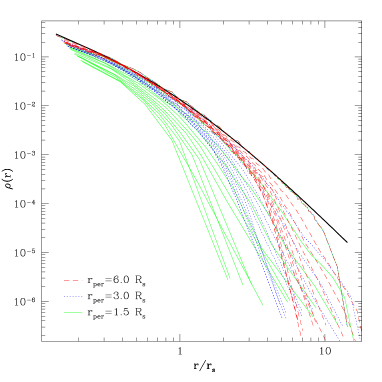
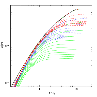
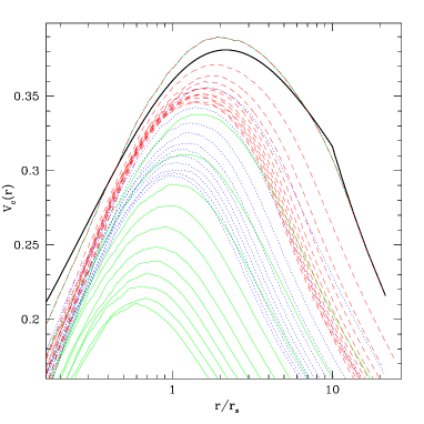
Figure 10.— Density, mass, and circular velocity profiles of the bound mass of $N=10^{5}$ satellite halos. Profiles are shown at apocenter for three different orbits with $r_{\rm ap}=10.0~{}R_{s}$ and $r_{\rm per}$ as shown. Density is given in units of $m_{\rm sat}/r_{s}^{3}$, mass is in units of $m_{\rm sat}$, and velocity is in units of $\sqrt{Gm_{\rm sat}/r_{s}}$. Thick solid curves correspond to the initial (unstripped) NFW profiles.

Figure 11.— Modified NFW profile fits to selected halo mass profiles from the middle panel of Figure 10. The dashed line shows the original, unstripped NFW mass profile. The parameters $r_{te}$ and $f_{t}$ control the truncation radius and the reduction in central density of the stripped profile, respectively.

Figure 12.— The peak circular velocity of stripped halos, $V_{\rm max}$ (top panel) in units of the initial peak circular velocity, as well as the parameters $f_{t}$ (middle panel) and $r_{te}$ (bottom panel), shown as a function of the remaining bound mass fraction $m_{\rm bnd}$. Solid curves show fits to the data given by $V_{\rm max}\propto m_{\rm bnd}^{1/3}$, and eqs. 9 and 10 for top, middle and bottom panels, respectively.

Figure 13.— Cumulative (peak) circular velocity function of substructure halos. Velocities are normalized to the circular velocity of the parent halo measured at the virial radius. The short-dashed curves correspond to two galaxy-sized halos formed in an SCDM universe (M99). Long-dashed curves correspond to a halo formed in the $\Lambda$CDM cosmogony (Font et al. 2001). The dot-dashed curve correspond to results reported by K99b. Curves with symbols correspond to the satellites observed around the Milky Way, using different assumptions to compute the peak circular velocity of their surrounding halos. Filled circles: Milky Way satellites assuming that stars in dwarf spheroidals are on isotropic orbits in isothermal potentials (as in M99) and that $V_{200}=220\>{\rm km}\,{\rm s}^{-1}$ for the Galaxy. Open circles: circular velocity at the luminous cutoff ($r_{tl}$) assuming that dwarf spheroidals are surrounded by dark halos with NFW profiles. Shaded region is bounded by peak circular velocity function of unstripped NFW halos assuming two extreme accretion redshifts, $z_{\rm acc}=10$ and $0$. See text for details.

Figure 14.— Circular velocity profiles of unstripped and stripped halos chosen to match the surface brightness profile and the stellar velocity dispersion of Carina (left panels) and Draco (right panels). Dashed curves show the circular velocity profiles of the corresponding halos before stripping. Upward vertical arrows indicate the luminous cutoff radius $r_{tl}$. The luminous cutoff radius shown for Draco is that of Odenkirchen et al. (2001), who find $r_{tl}=1020$ pc. Downward vertical arrows indicate the tidal radius $r_{te}$ corresponding to each of the stripped halos. Top and bottom panels show halo profiles adopting Eke, Navarro & Steinmetz (2001) NFW parameters corresponding to halos identified at $z=0$ and $5$, respectively.

References

- Aguilar and White (1985) Aguilar, L. A. and White, S. D. M.: 1985, ApJ 295, 374
- Avila-Reese et al. (2001) Avila-Reese, V., Colín, P., Valenzuela, O., D’Onghia, E., and Firmani, C.: 2001, ApJ 559, 516
- Bahcall et al. (1999) Bahcall, N. A., Ostriker, J. P., Perlmutter, S., and Steinhardt, P. J.: 1999, Science 284, 1481
- Benson et al. (2001) Benson, A. J., Frenk, C. S., Lacey, C. G., Baugh, C. M., and Cole, S.: 2001, Preprint [astro-ph/0108218]
- Bertschinger (1985) Bertschinger, E.: 1985, ApJS 58, 39
- Binney and Tremaine (1987) Binney, J. and Tremaine, S.: 1987, Galactic dynamics, Princeton, NJ, Princeton University Press
- Blumenthal et al. (1984) Blumenthal, G. R., Faber, S. M., Primack, J. R., and Rees, M. J.: 1984, Nature 311, 517
- Bode et al. (2001) Bode, P., Ostriker, J. P., and Turok, N.: 2001, ApJ 556, 93
- Bullock et al. (2000) Bullock, J. S., Kravtsov, A. V., and Weinberg, D. H.: 2000, ApJ 539, 517
- Burkert (1997) Burkert, A.: 1997, ApJ 474, L99
- Colín et al. (2000) Colín, P., Avila-Reese, V., and Valenzuela, O.: 2000, ApJ 542, 622
- Cole et al. (1994) Cole, S., Aragon-Salamanca, A., Frenk, C. S., Navarro, J. F., and Zepf, S. E.: 1994, MNRAS 271, 781
- Colpi et al. (1999) Colpi, M., Mayer, L., and Governato, F.: 1999, ApJ 525, 720
- Dalcanton and Hogan (2001) Dalcanton, J. J. and Hogan, C. J.: 2001, ApJ 561, 35
- Davis et al. (1985) Davis, M., Efstathiou, G., Frenk, C. S., and White, S. D. M.: 1985, ApJ 292, 371
- Dehnen (2001) Dehnen, W.: 2001, MNRAS 324, 273
- Dubinski and Carlberg (1991) Dubinski, J. and Carlberg, R. G.: 1991, ApJ 378, 496
- Efstathiou (1992) Efstathiou, G.: 1992, MNRAS 256, 43P
- Eke et al. (2001) Eke, V. R., Navarro, J. F., and Steinmetz, M.: 2001, ApJ 554, 114
- Font et al. (2001) Font, A. S., Navarro, J. F., Stadel, J., and Quinn, T.: 2001, ApJ 563, L1
- Frenk et al. (1988) Frenk, C. S., White, S. D. M., Davis, M., and Efstathiou, G.: 1988, ApJ 327, 507
- Fukushige and Makino (1997) Fukushige, T. and Makino, J.: 1997, ApJ 477, L9
- Ghigna et al. (1998) Ghigna, S., Moore, B., Governato, F., Lake, G., Quinn, T., and Stadel, J.: 1998, MNRAS 300, 146
- Ghigna et al. (2000) Ghigna, S., Moore, B., Governato, F., Lake, G., Quinn, T., and Stadel, J.: 2000, ApJ 544, 616
- Gnedin et al. (1999) Gnedin, O. Y., Lee, H. M., and Ostriker, J. P.: 1999, ApJ 522, 935
- Hernquist (1993) Hernquist, L.: 1993, ApJS 86, 389
- Irwin and Hatzidimitriou (1995) Irwin, M. and Hatzidimitriou, D.: 1995, MNRAS 277, 1354 (IH95)
- Kauffmann et al. (1993) Kauffmann, G., White, S. D. M., and Guiderdoni, B.: 1993, MNRAS 264, 201
- King (1962) King, I. R.: 1962, AJ 67, 471
- King (1966) King, I. R.: 1966, AJ 71, 64
- Kleyna et al. (2001) Kleyna, J. T., Wilkinson, M. I., Evans, N. W., and Gilmore, G.: 2001, ApJ 563, L115
- Klypin et al. (1999a) Klypin, A., Gottlöber, S., Kravtsov, A. V., and Khokhlov, A. M.: 1999a, ApJ 516, 530 (K99b)
- Klypin et al. (2001) Klypin, A., Kravtsov, A. V., Bullock, J. S., and Primack, J. R.: 2001, ApJ 554, 903
- Klypin et al. (1999b) Klypin, A., Kravtsov, A. V., Valenzuela, O., and Prada, F.: 1999b, ApJ 522, 82 (K99a)
- Knebe et al. (2002) Knebe, A., Devriendt, J. E. G., Mahmood, A., and Silk, J.: 2002, MNRAS 329, 813
- Majewski et al. (2000) Majewski, S. R., Ostheimer, J. C., Patterson, R. J., Kunkel, W. E., Johnston, K. V., and Geisler, D.: 2000, AJ 119, 760
- Mateo (1998) Mateo, M. L.: 1998, ARA&A 36, 435
- Mayer et al. (2001) Mayer, L., Governato, F., Colpi, M., Moore, B., Quinn, T., Wadsley, J., Stadel, J., and Lake, G.: 2001, ApJ 559, 754
- Moore et al. (2001) Moore, B., Calcáneo-Roldán, C., Stadel, J., Quinn, T., Lake, G., Ghigna, S., and Governato, F.: 2001, Phys. Rev. D 64, 063508
- Moore et al. (1999) Moore, B., Ghigna, S., Governato, F., Lake, G., Quinn, T., Stadel, J., and Tozzi, P.: 1999, ApJ 524, L19 (M99)
- Moore et al. (1998) Moore, B., Governato, F., Quinn, T., Stadel, J., and Lake, G.: 1998, ApJ 499, L5
- Moore et al. (1996) Moore, B., Katz, N., and Lake, G.: 1996, ApJ 457, 455
- Navarro (2002) Navarro, J. F.: 2002, in J. Makino and P.Hut (eds.), Astrophysical SuperComputing using Particles, IAU Symposium No. 208, Preprint [astro-ph/0110680]
- Navarro et al. (1996) Navarro, J. F., Frenk, C. S., and White, S. D. M.: 1996, ApJ 462, 563 (NFW)
- Navarro et al. (1997) Navarro, J. F., Frenk, C. S., and White, S. D. M.: 1997, ApJ 490, 493
- Odenkirchen et al. (2001) Odenkirchen, M., Grebel, E. K., Harbeck, D., Dehnen, W., Rix, H., Newberg, H. J., Yanny, B., Holtzman, J., Brinkmann, J., Chen, B., Csabai, I., Hayes, J. J. E., Hennessy, G., Hindsley, R. B., Ivezić, Ž., Kinney, E. K., Kleinman, S. J., Long, D., Lupton, R. H., Neilsen, E. H., Nitta, A., Snedden, S. A., and York, D. G.: 2001, AJ 122, 2538
- Peebles (1984) Peebles, P. J. E.: 1984, ApJ 277, 470
- Power et al. (2002) Power, C., Navarro, J. F., Jenkins, A., Frenk, C., White, S. D. M., Springel, V., Stadel, J., and Quinn, T.: 2002, Preprint [astro-ph/0201544]
- Quinlan (1996) Quinlan, G. D.: 1996, New Astronomy 1, 255
- Somerville (2001) Somerville, R. S.: 2001, Preprint [astro-ph/0107507]
- Spergel and Steinhardt (2000) Spergel, D. N. and Steinhardt, P. J.: 2000, Physical Review Letters 84, 3760
- Springel et al. (2001) Springel, V., White, S. D. M., Tormen, G., and Kauffmann, G.: 2001, MNRAS 328, 726
- Stadel (2001) Stadel, J. G.: 2001, Ph.D. thesis, University of Washington
- Stoehr et al. (2002) Stoehr, F., White, S. D. M., Tormen, G., and Springel, V.: 2002, Preprint [astro-ph/0203342]
- Taylor and Babul (2001) Taylor, J. E. and Babul, A.: 2001, ApJ 559, 716
- Tormen et al. (1998) Tormen, G., Diaferio, A., and Syer, D.: 1998, MNRAS 299, 728
- van Kampen (2000) van Kampen, E.: 2000, Preprint [astro-ph/0002027]
- Warren et al. (1992) Warren, M. S., Quinn, P. J., Salmon, J. K., and Zurek, W. H.: 1992, ApJ 399, 405
- White (2000) White, S. D. M.: 2000, ITP Conference on Galaxy Formation and Evolution, http://online.itp.ucsb.edu/online/galaxy/c00/white/
- White and Rees (1978) White, S. D. M. and Rees, M. J.: 1978, MNRAS 183, 341