Single Dish Calibration Techniques at Radio Wavelengths

Abstract

Calibrating telescope data is one of the most important issues an observer faces. In this chapter we describe a number of the methods which are commonly used to calibrate radio telescope data in the centimeter wavelength regime. This includes a discussion of the various methods often used in determining the temperature and gain of a telescope, as well as some of the more common difficulties which can be encountered.

NAIC/Arecibo Observatory, HC3 Box 53995, Arecibo, PR 00612; koneil@naic.edu

1. Introduction – The Importance of Calibration

As you likely know, every telescope is unique. One result of the uniqueness of individual telescopes is the difficulty of directly comparing measurements from one telescope with those from another. That is, Telescope A may record 280 counts for the peak of a given spectral line, while Telescope B may record only 100 counts. This is further complicated by the fact that even measurements taken on a given telescope, at a given frequency, can change over time. These changes can be the result of changes in, e.g. the telescope system temperature, the telescope response, and/or the atmospheric conditions. This means that even if you only observe your object with Telescope A, but measure it repeatedly over a year, you may discover that your object’s peak count varies from 280 one day to 250 or 300 on another day, and so forth. You then need to understand whether the source emission is truly varying with time or if the differences are due to changes within the telescope and equipment.

In order to compare measurements between two telescopes, or even between one telescope taken at different times, we need a universal measurement system. That is, we need to be able to state that 280 counts from Telescope A is equivalent to X counts from Telescope B or equivalent to Y counts from Telescope A at a different epoch. This is the process of data (or telescope) calibration, and the rest of this chapter will be devoted to presenting the various methods available, both observationally and theoretically, to calibrate data.

2. A Brief Review

At this point it is useful to go over the more important equations and concepts that are used in the calibration process. All of these topics are also covered in other chapters, where more detailed discussions can be found.

2.1. The Rayleigh-Jeans Approximation

Recall that the Planck Law for blackbody radiation is

$$\rm B\>=\>{{2h\nu^{3}}\over{c^{2}}}\>{{1}\over{e^{h\nu/kT}-1}}$$ (1)

where B is the brightness (specific intensity) measured in W/m²/Hz/rad² (or Jy/rad²); h is Planck’s constant (6.63 $\times 10^{-34}$ Js); $\nu$ is the frequency in Hz; k is Boltzman’s constant (1.38$\times 10^{-23}$ J/K); and T is the temperature, in K. In the centimeter wavelength regime, it is often true that h$\nu\>\ll$ kT. In this case, you can use the Taylor Series to expand $e^{h\nu/kT}-1$. This provides the Rayleigh-Jeans approximation for blackbody radiation at radio wavelengths:

$$\rm B\>=\>{{2kT\nu^{2}}\over{c^{2}}}\>=\>{{2kT}\over{\lambda^{2}}}\>.$$ (2)

For a discrete radio source of temperature T and subtending a solid angle $\Omega_{S}$ the source flux density (S) in the Rayleigh-Jeans limit is obtained by integrating over the source solid angle:

$$\rm S\>=\>{{2k}\over{\lambda^{2}}}\>\int_{\Omega_{S}}{T(\theta,\phi)d\Omega}\>.$$ (3)

If the brightness temperature of the source is uniform across $\Omega_{S}$, this reduces to

$$\rm S\>=\>{{2kT}\over{\lambda^{2}}}\>\Omega_{S}\>.$$ (4)

2.2. Antenna Temperature

The antenna temperature (T_A) can be defined as the temperature of the antenna radiation resistance. That is, let the telescope observe a point source (i.e. a source which is considerably smaller than the beam size) which has a flux density S. Then, replace the feed of the telescope with a matched resistor (or load). If you now adjust the temperature of the resistor until the power received is the same as it was for the point source (observed with the antenna or feed horn), the antenna temperature is equal to the resistor temperature. That is, the measured spectral power is simply w=kT_A.

If absorbing matter is present, or the source does not completely fill the beam, the measured antenna temperature will be less than the source temperature. In this case you will measure an antenna temperature T_A and you have

$$\rm w\>=\>kT_{A}$$ (5)

$$\rm S\>=\>{{2kT_{A}}\over{\lambda^{2}}}\Omega_{A}\>=\>{{2kT_{A}}\over{A_{e}}}\>$$ (6)

$$\rm w\>=\>{1\over 2}{A_{e}}S\;.$$ (7)

Here, A_e is the effective aperture of the antenna, and $\Omega_{A}$ is the solid angle of the telescope power pattern. Recall that the antenna theorem gives A${}_{e}\>\Omega_{A}\>=\>\lambda^{2}$ or, if ohmic losses are considered, A${}_{e}\>\Omega_{A}\>=\>\epsilon_{r}=;\lambda^{2}$, where $\epsilon_{r}$ is the fractional power transmission of the antenna, typically close to unity. (See the the chapters by, i.e. Hagen or Goldsmith for further derivation of this quantity.)

In practice, the antenna temperature is given by

$$\rm T_{A}\>=\>{{A_{e}}\over{\lambda^{2}}}\int{\int{T_{source}(\theta,\phi)P_{n}(\theta,\phi)d\Omega}}\>=\>{{\epsilon_{r}}\over{\Omega_{A}}}\int{\int{T_{source}(\theta,\phi)P_{n}(\theta,\phi)d\Omega}}\>.$$ (8)

Here $\Omega_{A}$ is again the antenna solid angle and P${}_{n}(\theta,\phi)$ is the antenna power pattern (normalized to unity at maximum). If the source is a true “point source”, i.e. it is small compared to the beam size, $P_{n}(\theta,\phi)\>\sim$ 1 over the source solid angle and

$$\rm T_{A}\>\approx\>{{\epsilon_{r}}\over{\Omega_{A}}}\int{\int_{\Omega_{S}}{T_{source}d\Omega}}\>=\>\epsilon_{R}\;{{\Omega_{S}}\over{\Omega_{A}}}\>T_{avg}$$ (9)

where $\rm T_{avg}$ is the brightness temperature averaged over the source. If, on the other hand, the source is large compared to the beam size and has a constant brightness temperature T_const, the antenna temperature is

$$\rm T_{A}\>=\>{{\epsilon_{r}T_{const}}\over{\Omega_{A}}}\int{\int_{source}{P_{n}(\theta,\phi)d\Omega}}\>=\>{{T_{const}}\over{\Omega_{A}}}\>\Omega_{b}^{\prime}\epsilon_{r}\>.$$ (10)

Here, $\Omega_{b}^{\prime}$ is the solid angle subtended by both the main beam and the side lobes falling on the source. (Note that if the source just fills the main beam, $\Omega_{b}^{\prime}$ = $\Omega_{m}^{\prime}$, the main beam solid angle.) Finally, if the source fills the sky ($\Omega_{S}\>\gg$ beam size), T_A = $\rm\epsilon_{r}$ T_const.

2.3. Minimum Detectable Temperature and Flux Density

The minimum detectable antenna temperature is set by the fluctuations in the receiver output caused by the system noise. As has been discussed in other chapters, this noise is directly proportional to the system temperature (T_sys). T_sys can be broken down into three parts for analysis – the antenna contribution (T_A), the receiver contribution (T_R), and the power loss between the two. More specifically, the system temperature can be written as

$$\rm T_{sys}\>=\>T_{A}\>+\;T_{LP}\left[1/\epsilon\>-\>1\right]\>+\>\left(1/\epsilon\right)\>T_{R}$$ (11)

where T_LP is the physical temperature of the transmission line between the antenna and the receiver, and $\epsilon$ is the efficiency of the transmission (0 $\leq\>\epsilon\>\leq$ 1). The sensitivity of a radio telescope is then equal to the rms noise fluctuations of the system:

$$\rm\Delta T_{rms}\>=\>{{K_{S}T_{sys}}\over{\sqrt{\Delta\nu\;t\;n}}}.$$ (12)

Here, $K_{S}$ is the sensitivity constant of the telescope (dimensionless and of order unity), $\Delta\nu$ is the pre-detection bandwidth (in Hz), t is the integration time for one record (in s), and n is the number of records averaged (dimensionless). The minimum detectable temperature is typically considered to be 3–5 times the rms noise temperature (e.g. $\rm\Delta T_{min}\>=\>3T_{rms}$).

The minimum detectable temperature can be converted to a minimum brightness or flux density by applying the Rayleigh-Jeans approximation (Equations 2 and 7):

$$\rm\Delta B_{rms}\;=\;{{2k}\over\lambda^{2}}\;{{K_{S}T_{sys}}\over{\sqrt{\Delta\nu\;t\;n}}}$$ (13)

$$\rm\Delta S_{rms}\;=\;{{2k}\over A_{e}}\;{{K_{S}T_{sys}}\over{\sqrt{\Delta\nu\;t\;n}}}\>.$$ (14)

3. System Temperature

System temperature, for the purpose of this chapter, will be defined by breaking it into two parts:

$$\rm T_{sys}(\alpha,\delta,az,za)\>=\>T_{off}(\alpha,\delta,az,za)\>+\>T_{source}(\alpha,\delta,az,za)$$ (15)

where $\alpha,\delta,az,za$ are the source right ascension, source declination, and telescope position in azimuth and zenith angle, respectively. The “off source” temperature is simply the temperature measured if the telescope were pointed at a nearby region of blank sky:

$$\rm T_{off}(\alpha,\delta,az,za)\>=\>T_{RX}\>+\>T_{gr}(za,az)\>+\>T_{atm}(za)\>+\>T_{CMB}\>+\>T_{BG}(\alpha,\delta)\;.$$ (16)

T_RX is the receiver temperature; T_gr the temperature contributed from the ground; T_atm the contribution from the atmosphere; $T\rm_{CMB}$ the contribution from the cosmic microwave background; and $\rm T_{BG}$ the contribution from background and foreground celestial sources, including Galactic emission.

Theoretically, the system temperature of a telescope changes with telescope elevation due to atmospheric emission following:

$$\rm T_{atm}\>=\>T\left({1\;-\;e^{-\tau A}}\right)\;,$$ (17)

where $\tau$ is the atmospheric opacity at zenith and A is related to the zenith angle at which the telescope is pointing (A = sec(za)). A well-built telescope with an unblocked (or partially blocked) aperture and a raised, movable dish can come close to achieving this theoretical model (Figure 1). In reality, though, a number of factors must be added to this theoretical model. In particular, most telescopes experience temperature changes due to changes in the ground radiation with elevation, reflection of radiation (both atmospheric and celestial) off the telescope structure, and changes in the system itself.

Figure 1.: System temperature for the Green Bank Telescope as measured at 2 GHz on 21-22 March, 2001. (From Ghigo, Maddalena, Balser, & Langston 2001.)

In practice, the source temperature can be separated from the system temperature by making two observations – one which includes the source in the beam (the ON), and one which does not (the OFF). The source temperature is then just:

$$\rm T_{Source}\>=\>{T_{ON}\;-\;T_{OFF}}$$ (18)

$$\rm{T_{Source}\over T_{off}}\>=\>{{T_{ON}\;-\;T_{OFF}}\over{T_{OFF}}}$$ (19)

$$\rm T_{Source}\>=\>\left[{{T_{ON}\;-\;T_{OFF}}\over{T_{OFF}}}\right]\;T_{off}\>$$ (20)

where $\rm T_{ON}$ and $\rm T_{OFF}$ are the power measurements for the two celestial positions.

At this point it should be clear that one of the most important measurements to be made in order to understand, and calibrate, your data is the measurement of system temperature. In the regime of centimeter wavelength astronomy there are two techniques commonly used to make this determination. These will be discussed in the next section.

3.1. Switched Noise Diode

The first technique for measuring system temperature uses a “switched noise diode”. With this method, a noise diode with known effective temperature at the desired frequency is coupled to the telescope system (Figure 2). The telescope is then pointed to the blank sky and two measurements are made – one with the diode turned on ($\rm ON_{CAL}$) and one with the diode turned off ($\rm OFF_{CAL}$). These measurements are then used to determine the off-source system temperature, T_off.

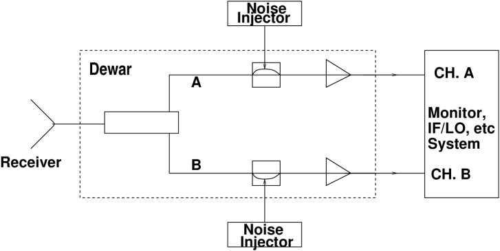
Figure 2.: Schematic drawing of the noise diode injection into a receiver system. This schematic is modeled after the L-Narrow receiver system at Arecibo Observatory.

The basis behind the switched noise diode technique is quite simple. The $\rm ON_{CAL}$ measurement is simply the sum of the system temperature plus the effective temperature of the diode, while the $\rm OFF_{CAL}$ observation, in theory, measures only the system temperature. The system temperature can then be derived by comparing the temperature of the noise diode, measured as a fraction of the system temperature, with the known temperature of the noise diode. In other words, system temperature is

$$\rm{{T_{off}}\over{T_{cal}}}\>=\>{{OFF_{CAL}}\over{{ON_{CAL}}\;-\>OFF_{CAL}}}$$ (21)

$$\rm T_{off}(K)\>=\>{{OFF_{CAL}}\over{ON_{CAL}\;-\>OFF_{CAL}}}\>\times\>{\left[{T_{cal}(K)}\;\right]}_{known}$$ (22)

Although in theory switched noise diodes provide an excellent tool for measuring the system temperature, in practice a number of difficulties exist which limit the accuracy of the noise diode method. The first complication is that the effective temperatures of most diodes have a frequency dependence. This is not an overwhelming complication, as one can either obtain temperature measurements at a variety of frequencies or use some other multi-frequency calibration methods (i.e. van Zee, et al. 1997). It is merely an added issue to be aware of when determining or applying noise diode measurements to your data.

A second issue to consider when using noise diodes to determine the system temperature is the time stability of the diodes. A good (well-built) noise diode, in a well controlled environment, should remain stable for a number of years. Yet the performance of a diode should be checked by frequent (bi-annual or more often) measurements of the diode response across the frequency band of interest, to insure that the diode is performing according to its specifications.

The final issue to consider when using the noise diode system is the accuracy of the measurement of the noise diode response. This is a non-trivial issue, as noise diode measurements are typically determined through bootstrapping off another (‘standard’) noise diode, which is believed to have a well-known, accurately measured value. Noise diode measurements therefore start off with an initial error from the measurement of the standard diode. As all other measurements are done through bootstrapping off the first diode measurement, this initial error is then propagated throughout all measurements. Added to the initial measurement errors are, of course, the errors inherent in the measurement process itself. Finally, it should be remembered that the initial noise diode measurements (that is, the measurements coming from the standard diode comparison) are not temperature measurements, but instead most be converted from, i.e. a voltage measurement, and in that process yet more error is introduced.

In sum, the errors introduced just by the measurements of the noise diode value are:

$$\rm\sigma_{total}\>=\>\sqrt{\sigma^{2}_{freq.\;dependence}\;+\;\sigma^{2}_{stability}\;+\;\sigma^{2}_{measured\;value}\;+\;\sigma^{2}_{conversion\;error}}$$ (23)

where

$$\rm\sigma_{measure\;value}\>=\>\sqrt{\sigma^{2}_{standard\;cal}\;+\;\sigma^{2}_{instrumental\;error}\;+\;\sigma^{2}_{loss\;uncertainties}}$$ (24)

In spite of these difficulties, though, noise diodes can give a fairly accurate indication of a telescope’s system temperature, often to within 2% or less.

Note – System temperature is often measured at telescopes using a method known as the “Y-Factor” method. This method employs two diodes (or similar sources) of known effective temperatures and does not include any effects of the antenna. If diode one has a known effective temperature T₁ and diode two has a known effective temperature T₂, the ratio of the measured power of the two diodes will be

$$\rm Y\>=\>{{T_{1}\;+\;T_{off}}\over{T_{2}\;+\;T_{off}}}$$ (25)

where recall T_off for these purposes is the system temperature without any effect of the antenna. This ratio (the Y-Factor) can then be used to obtain T_off via

$$\rm T_{off}\>=\>{{T_{1}\;-Y\;T_{2}}\over{Y\;-\;1}}\;.$$ (26)

3.2. Hot & Cold Loads

Another method for obtaining the system temperature is through the use of hot and cold loads. A cold load is typically an absorbing system placed inside some gas or liquid at a known temperature (often liquid Nitrogen). This load is then placed over, or otherwise coupled with, the receiver of choice, and the power level is measured. The hot load is often a similar measurement of a load at ambient temperature. Alternatively, the ‘cold’ load can be a blank sky measurement and the hot load can be a measurement of a load placed inside a liquid of known temperature. These measurements can then be used in the same fashion as a noise diode to obtain the system temperature.

Measuring the system temperature using hot and cold loads can be considerably more reliable than the noise diode method. The primary reasons for the superiority of the hot/cold load method are that the temperature of the loads can be measured directly, and the measurements are all temperature measurements – no conversions are necessary. However, the hot/cold load system is not used at most centimeter wavelength radio telescope as building loads large enough to encompass a $\lambda\>>$ 5–6 cm feed, and which have the easy availability necessary for on-the-fly measurements is highly impractical. As a result, the use of hot/cold loads to measure system temperature on-the-fly is generally restricted to the $\lambda\><$ 5–6 cm regime. In the $\lambda\>>$ 5–6 cm regime, hot/cold loads are often used to check the noise diode measurements from the switched noise diode technique (and can be used in place of a standard diode for calibration, as is the case at the Green Bank Telescope). A more detailed discussion of this, and similar, calibration methods at short wavelengths is given elsewhere in this book.

4. Off-Source Observations

In Section 3 we showed that the temperature of the object of interest can be found by measuring the system temperature and using that measurement in combination with a blank-sky measurement of T_sys, to calibrate the observations. That is equation 20 gave:

$$\rm T_{source}(K)\>=\>\left[{{T_{ON}\;-\>T_{OFF}}\over{T_{OFF}}}\right]\;T_{off}(K)$$ (27)

As Section 3 discussed the various means for determining the system temperature, the next step is to determine the best method for obtaining an appropriate off-source, or blank sky, observation.

4.1. Baseline Fitting

Baseline fitting to just the on-source records is potentially the simplest and most efficient of the methods for obtaining blank sky information for spectroscopic observations. The idea is straightforward – a baseline is fit to those spectral regions of an observation which are known to contain no signal from the object of interest. This baseline is then treated as the off source (blank sky) observation (Figure 3a).

Figure 3.: Examples showing successful fitting of a flat baseline to an observation (left), and an observation in which baseline fitting is not a viable option (right – courtesy of C. Conselice). Both images include the spectral line of interest and a number of ‘blank’ channels.

Although this procedure is extremely efficient, it has several drawbacks. In particular, it is not a feasible option if the spectral line of interest is large compared to the bandpass (that is, if there are too few channels from which to fit a reasonable baseline), or if there is are standing waves present which have a frequency higher than, or of order of, the bandpass of interest. Additionally, if the baseline is not reasonably flat for any reason this option should not be used, as a poor fit can artificially add or subtract considerable emission to the line of interest (Figure 3b).

Errors induced from the baseline fitting method come primarily from the quality of fit.

4.2. Frequency Switching

The frequency switching technique obtains blank sky information by keeping the telescope pointed at the object of interest, but switching the center frequency of the measurements (changing the frequency of the first local oscillator). As this mode of observing does not require any movement of the telescope, it can be done very quickly and efficiently. When the data from the two settings are subtracted, the quasi-stationary effects introduced into the data after the first mixer, such as spectral ripples, are cancelled. Additionally, if the frequency is shifted such that the frequency range of interest remains within the bandpass, but does not overlap its original “unswitched” range, frequency switching can be made extremely efficient (Figure 4). Liszt (1997) describes a deconvolution method for the case in which the two ranges do overlap.

Frequency switching has a number of advantages over the baseline fitting method. First, frequency switching reduces the chance of error induced though poor fits to the baselines in the regions of interest. Second, frequency switching can allow for higher resolution spectra as considerable bandpass does not need to be ‘wasted’ to accommodate a large number of blank channels, as is typically necessary for baseline fitting. Finally, because frequency switching can occur at a very rapid rate (on the order of a second, or less), frequency switching can cancel any post-mixer variations on this, or longer, time scales.

Figure 4.: Data taken in frequency switching mode. The center line denotes the separation between the two images. Here the x-axis is channels and the y-axis in raw counts. As the spectral line of interest is available in both images, it would be possible to fold the data back together to achieve a higher signal to noise (and better observing efficiency).

The disadvantages to frequency switching at centimeter wavelengths are few. The primary difficulties are that (a) the redshift of the line of interest must be accurately known a priori; (b) the system must be stable enough that the baselines of the primary observation and the frequency switched observation are virtually identical; and (c) as with baseline fitting, if there are significant standing waves in the baseline due to reflections off the telescope structure for a partially blocked aperture or the presence of strong continuum source within the beam, frequency switching may be unable to eliminate the standing pattern (provided, of course, the characteristic frequency is not considerably wider than the frequency shift).

4.3. Position Switching

Position switching involves observing the object of interest for a fixed period of time, and then moving the telescope to a blank sky region to obtain the blank sky observations necessary for baseline subtraction. Although costly in terms of telescope time, this observing method has the advantages that no a priori information (other than position and a redshift known well enough that the line of interest will lie within the spectrometer bandpass) need to be known about the object and continuum emission within the beam can be less of a problem (although see Section 4.4, below).

There are a number of issues to consider when deciding to use position switching. The first consideration is the time stability of the telescope and baselines. As position switching typically requires re-pointing the telescope, it is not feasible to switch between the on-source and blank-sky observations at a rapid rate (although see the sections on wobbler switching and chopper wheel techniques in the chapter by Jewell). This means the telescope baselines must remain stable over a reasonable period of time, where this period of time is defined by the amount of time it takes to observe both the on and off-source positions. (That is, if five minute on- and off-source observations are being taken, with one minute between the observations, the baselines must be stable for at least 11-12 minutes, if not considerably longer.)

A second issue which needs to be considered when performing position switched observations is the dish illumination and aperture blockage. If the same portion of the dish is not illuminated during the on- and off-source observations, large differences in the baselines can be present. This is particularly true if there are significant standing waves in the baseline due to a partially blocked aperture. These difficulties are extreme for a telescope like the Arecibo 305-m which has a fixed primarily reflector. In this case, observations of different sky positions may not only illuminate different areas of the reflector but can also have markedly different contributions from reflections off the ground and telescope structure. In this case it is prudent to obtain the off-source observation by tracking a blank sky region chosen such that the illumination pattern of the feed tracks across the same part of the primary reflector as for the on-source observation. In this case, if a five minute on-source observation of an object was taken, starting when the object was at an Azimuth of 283^∘and Zenith angle of 13^∘, the off-source observation should also last for five minutes and start at AZ , ZA = (283^∘, 13^∘). Although this method is time consuming, it can offer considerably flatter the baselines and therefore a considerable reduction in the spectral deviations introduced by the system.

The final issue to consider with position switching is that, if the size of the source is considerably more extended in angular distance than the difference between the on and off-source sky positions (as is the case for the ubiquitous Galactic HI), position switching becomes an impractical option. In these cases other alternatives such as frequency switching, baseline fitting, etc. must be considered.

4.4. Variations

To get around some of the difficulties inherent in the above ‘standard’ procedures for obtaining off-source observations, a number of variations of these methods have been (and are constantly being) devised. In this section we enumerate a few of these methods which have proven to be useful.

Baseline Fitting with an Average Fit

One method for reducing random noise which can cause difficulties when fitting a function to the baselines (Section 4.1) is to average, or median average, all the observations together and use that average to determine the baseline fit for the data. This has the advantage of providing a fairly accurate baseline, but at the expense of losing detailed information which may be important in individual fits, particularly if the time over which the average is taken is longer than the stability time of the telescope system.

Position Switching on an Extended Source

As was mentioned in Section 4.3, the position switching method is not easily applied when observing a source which is extended when compared with the offset distance between the on-source and off-source observations. Although frequency switching is typically the preferred observing method in these cases, occasionally it is not a viable option. In these cases, an alternative observing method must be considered. One option which can be used when mapping an extended, but finite, source is to extend the map beyond the edges of the source. The desired blank sky information is then obtained by averaging the off-source observations or by fitting baselines across the map using the off-source observations (Figure 5).

Figure 5.: Diagram showing the off-source regions typically used to obtain blank sky information, using position switching, for an extended source.

If the telescope being used does not have a constant telescope illumination as it points to different sky positions, such as is the case for the Arecibo 305-m telescope, it is often useful to use only those observations at a given Right Ascension (if the map is stepping in Declination – at a given Declination otherwise) to obtain the best blank sky information. Even flatter baselines can be obtained in this case through drift-scan mapping, as in this method the off- and on-source observations are taken at the same (az,za).

Position Switching in the Presence of Continuum Emission

When position switching is attempted on a source with considerable continuum emission (T_source is a significant fraction of the value of T_sys), a markedly different standing wave amplitude can be observed in the baselines between the on- and off-source observations. As a result, the components of the standing wave pattern produced by the strong continuum emitter is not cancelled by the off-source observation. This problem is particularly noticeable in telescopes with partially blocked apertures and which have significant standing waves even in the blank sky observations.

One method for dealing with this problem is to observe another continuum source, of similar strength to the object of interest, and then to divide the source difference (ON $-$ OFF) spectrum by the reference difference spectrum to eliminate the residual standing waves. The result is a spectrum with a magnitude proportional to the ratio of the target and reference flux densities, and includes any spectral-line component (emission or absorption) that may be present in the target:

$$\rm R\>=\>{{\left({ON(\nu)\;-\;OFF(\nu)}\right)_{source1}}\over{\left({ON(\nu)\;-\;OFF(\nu)}\right)_{source2}}}$$ (28)

In this case, the rms noise on the observed ratio is:

$$\rm\sigma(R)\>=\>{{\sqrt{2}R}\over{\sqrt{\beta\tau}}}\>\times\;\left[\begin{array}[]{l}{{SEFD^{2}_{S1,ON}\;+\;SEFD^{2}_{S1,OFF}}\over{(SEFD_{S1,ON}\;-\;SEFD_{S1,OFF})^{2}}}\\ \\ \;+\;{{SEFD^{2}_{S2,ON}\;+\;SEFD^{2}_{S2,OFF}}\over{(SEFD_{S2,ON}\;-\;SEFD_{S2,OFF})^{2}}}\end{array}\right]^{1/2}$$ (29)

where S₁ and S₂ are continuum source one and two, respectively, and SEFD is the system equivalent flux density of the telescope, which is equal to the system temperature divided by the telescope gain at the frequency of interest. This method has been carefully tested at Arecibo Observatory, where the unique design of the 305-m telescope makes eliminating standing waves from the baselines a challenge. The results show that, although this method of ‘double position switching’ and obtaining the ratio of target flux densities initially increases the rms noise when compared to standard position switched observations, the noise decreases as 1/$\sqrt{time}$ with continued observation, while the noise of the standard position switched observations ceases to decrease after only four observation cycles have been averaged (Figure 6). Further information on this method can be found in Salter & Ghosh (2001), and references therein.

Figure 6.: The average of three typical observing cycles with a strong continuum source; (A) is for the standard position switching technique, (B) is double position switching by dividing the [ON – OFF]/OFF of the source with that of the reference spectra, and (C) is double position switching using the double position switching method discussed in Section 4.4. (Figure from Salter & Ghosh 2001.)

5. Flux Density Conversion

At this point we have discussed both steps necessary for converting observed (raw) data into units of antenna temperature. Although this is a significant step towards making data comparable between telescopes, it is not the complete picture. The reason for this is that every telescope has a different response, or gain. To complicate matters further, individual telescopes also have different gains at different frequencies or even different elevation angles. As a result, the temperature of a source must be converted from observed antenna temperature to a gain-corrected measurement. In radio astronomy this final, gain-corrected measurement is typically in units of flux density per beam or main beam brightness. Main beam brightness is simply the temperature measurement corrected for telescope efficiency ($\rm T_{MB}\>=\>\eta_{beam}T_{measured}$). As defined in Section 2, flux density per beam, on the other hand, is the integral of the source brightness over the telescope beam

$$\rm S\>=\>{{2k}\over{\lambda^{2}}}\;{{\int{\int{T(\theta,\phi)\;P_{n}(\theta,\phi)\;d\Omega}}}\over{\int{\int{P_{n}(\theta,\phi)\;d\Omega}}}}$$ (30)

The unit of flux density is W m^-2 Hz^-1, or Janskies (Jy) (1 Jy = 10^-22 W m^-2 Hz^-1).

As flux density per beam is the commonly used brightness units for most centimeter wavelength radio astronomy, the rest of the discussion in this section will concentrate on calibrating data into flux density units. If conversion into main beam brightness is instead desired, the overall methods are the same.

5.1. The Ideal Telescope

In an ideal telescope – one with a completely unblocked aperture, no ground reflection, lossless instrumentation, cables, etc., and a transparent atmosphere – the telescope gain can readily be theoretically modeled. Even in the case of a fairly simple and well understood system with minimum aperture blockage, an accurate theoretical prediction of the telescope’s gain can be obtained. (See, e.g. the discussions by Lockman and Condon in this book).

As discussed by both Condon and Salter (this book), if a telescope’s response can be well modeled, the telescope can be used to obtain absolute flux densities of continuum sources. Then, if the absolute flux densities of a reasonable number of continuum sources are determined at a variety of frequencies, monitored, and recorded, a catalog of ‘standard’ continuum sources can be developed. These sources can then be used to monitor telescope performance and look for any degradation in the telescope gain due to deterioration in the system components, distortion of the reflector shape, etc.

5.2. Bootstrapping

For many telescopes, determining a telescope’s gain theoretically is extremely complicated due to considerable or irregular blockage of the aperture, uncertain losses in the cabling or electronics, uneven reflection from the ground, etc. In these cases, rather than relying upon what could be fairly inaccurate models of the telescope gain, it is often good to take advantage of pre-existing catalogs of standard continuum source flux densities and “bootstrap” off those values to determine the gain of the telescope of interest.

When choosing which sources to observe from source catalogs, a few issues should be considered. First, the size of the chosen source should be small when compared with the size of telescope beam. If the source is of significant size when compared to the beam (a diameter more than $\sim$1/10 the telescope beam at the frequency of interest), issues such as the detailed beam pattern and potential spillover of the source onto the ground need be considered. These problems can be eliminated by insuring that the source is essentially point-like when compared to the beam.

The second item to consider when choosing a source for telescope gain calibration is that the source should be strong enough to supply a fairly high signal-to-noise ratio but not so strong as to cause difficulties with baseline ripples or the telescope’s dynamic range.

Finally, a good calibrator source should have a non-variable flux density which has been well determined at the frequency of interest. For a well defined telescope, errors in the previously determined flux density measurements typically dominate all other errors inherent in determining a telescope’s gain using the bootstrap technique. This means that reducing the errors in the pre-determined flux density values results in an essentially linear reduction in the errors in the telescope gain determination. One of the results of this is that the error in determining of a telescope’s gain (when obtained through bootstrapping) can be greatly reduced by observing a number of sources at a range of positions in the sky.

The primary difficulty with using the bootstrap technique to determine telescope gain is that if a telescope’s gain changes significantly at different sky positions, or if the telescope’s beam illumination or aperture blockage changes as the telescope points to different azimuth and/or zenith angles, it can readily become impractical for an observer to continuously monitor the telescope gain. It may take more time to determine the gain than to obtain the desired observations of the observer’s source. In this case, the observer often needs to rely on a telescope’s pre-determined standard gain curves.

5.3. Gain Curves

When not available through theoretical models, gain curves are obtained by observing a large number of standard flux density calibrators located across a telescope’s visible sky region at frequencies which range across the telescope’s usable bandwidth. Gain curves can be extremely useful if a telescope’s response is fairly stable over time and the gain of a telescope varies across the sky.

A telescope with an evenly illuminated reflector typically has a gain curve which varies with telescope zenith angle in a fairly predictable manner (Figure 7). Telescope gains can, though, become fairly complicated as aperture blockage is increased, the illuminated portion of the main reflector changes (as is the case with the Arecibo telescope), and the contribution from ground reflection changes. In this case it is possible to obtain gain curves which vary as the telescope moves in azimuth as well as zenith angle (Figure 8).

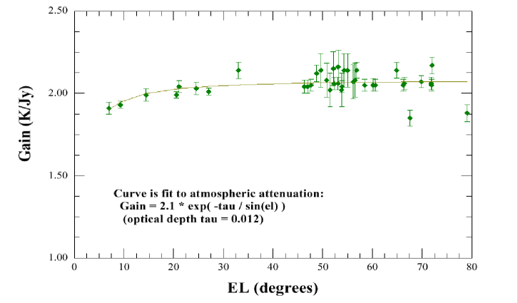
Figure 7.: Gain curve for the Green Bank Telescope. (From Ghigo, et al. 2001.)

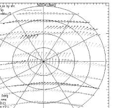
Figure 8.: Gain distribution for the Arecibo 305-m telescope. Here the both the length and angle of the arrow are proportional to the value of the gain, and the polar plot is in terms of zenith angle (radius) and azimuth angle ($\theta$).

Although the existence of pre-determined gain curves can save the observer a considerable amount of telescope time, gain curves should never be blindly accepted. Instead, a circumspect observer should recognize that although the shape of a telescope’s gain curve should remain relatively constant, a scaling of the curve may be necessary in the case of poor telescope focus, pointing offsets, or degradation in the feed, electronics, cabling, etc. As a result, it is always useful to obtain observations of a number of flux-density standards at telescope positions near those of the objects of interest. These observations can then be used to check the telescope gain curve and, when necessary, to scale the curve accordingly.

6. Other Issues

There are a variety of other issues which can affect the gain and system temperature of a radio telescope. In this section we will describe the more common issues an observer might encounter.

6.1. Pointing and Focus

Poor pointing or axial focus of a telescope can result in a reduction of the telescope gain. The reason for this is that a typical telescope main beam pattern is Gaussian in nature (to a fairly low level). As a result, a relatively offset in pointing can result in a significant reduction of the telescope gain at the position of the object (Figure 9a). In this case the signal-to-noise and calibration of the the observation can suffer severely. In a similar manner, poor telescope focus will artificially diffuse an object so that less of the object falls onto the center of the beam where the telescope gain is at the highest (Figure 9b). Again this will result in a degradation in the object signal-to-noise ratio.

The method for checking axial focus is telescope dependent. One reliable method for determining a telescope’s pointing is by performing cross-scans across a strong, point-like continuum source with an accurately known position. If a telescope’s pointing is accurate, the maxima of the scans will lie in the center of each cross scan. If the pointing is in error, an offset between the center of the cross scans and the peak intensity measured by the observation will be seen. In many cases, this offset can then be fed back into the telescope pointing model.

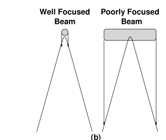
Figure 9.: Figure showing the results of (a) pointing errors and (b) focus errors on the measured flux of an object.

6.2. Side Lobes

Issues of side lobes in a telescope’s beam pattern are discussed extensively elsewhere in this book. (See, e.g., the contribution by Lockman.) However, as the presence of side lobes can affect the calibration of an observation, it is worthy of a brief mention here.

Because they can allow extraneous radiation to enter into an observation, the presence of side lobes in a telescope’s response pattern can artificially increase the measured flux from a source. This can result both in inaccurate measurements of a source’s flux density and, if a telescope’s gain is determined through bootstrapping, can create avoidable errors in the telescope’s gain determination. As a result, an observer should be aware of the presence and extent of a telescope’s side lobes at the frequency of interest. If possible, an observer should simply avoid observing any sky position where the side lobe contributions will cause unacceptable errors in the flux density measurements. When this is not possible (much of the time, particularly when mapping an extended source), the observer should attempt to use models of the side lobes and beam pattern to deconvolve the side lobe contributions from the desired spectrum.

6.3. Coma & Astigmatism

If a telescope’s feed or secondary reflector is displaced or rotated from its principal axis it will cause asymmetries in the detailed telescope beam. If a sub-reflector is shifted perpendicular off the main reflector axis, a pointing error is generated. This is known as a comatic error. Astigmatism occurs due to deformations in the reflector(s) and results in irregularities (or lobes) on the beam pattern (Figure 10). As with side lobes, the presence of distortions in a telescope beam pattern can artificially increase the measured flux density of an extended source due to the addition of stray radiation, and decrease the flux density for a point source (due to decreased telescope efficiency).

Figure 10.: Beam response for the Arecibo 305-m telescope. The contours are labeled in units of percent peak intensity and are spaced by 0.4%. The dotted cross marks the position of intensity maximum. The asymmetry in the beam pattern at the left of the image is due in large part to the effects of the coma. (From Heiles, et.al 2001).

7. Useful Resources

In this section we list a few of the resources that are useful when calibrating radio astronomy data.

• Baars, Genzel, Pauliny-Toth, & Witzel, 1977 A&A 61, 99
  

• Baars 1973 IEEE Trans. Trans. Antenna & Propagation, AP-21, No. 4, pp. 461–474
  

• Condon, et al. 1998, AJ, 115, 1693
  

• Kraus, Radio Astronomy 1986 (Ohio:Cygnus-Quasar Books)
  

• Kuhr, Witzel, Pauliny-Toth, & Nauber, 1981 A&AS 45, 367
  

• Northern VLA Sky Survey, online at http://www.cv.nrao.edu/NVSS
  

• Ott, et al. 1994 A&A 284, 331
  

• Tabara & Inoue 1980 A&AS 39, 379
  

Acknowledgments.

Thanks to Chris Salter and Ron Maddalena for their helpful comments on this paper, and of course many thanks to Paul M. for all his help.

References

Ghigo, F., Maddalena, R., Balser, D., & Langston, G. 2001 GBT Commissioning Memo #10

Heiles, C., et.al 2001 PASP, in press

Liszt, H. 1997 A&A 124, 183

Salter, C.J. & Ghosh, T. 2001 AAS 198, 7502

van Zee, L., et al. 1997 AJ 113, 1631