Numerical Simulations of Magnetic Fields
in Astrophysical Turbulence
Invited Review to be published in the Proceedings of the Workshop on Simulations of MHD Turbulence in Astrophysics, Paris, France, July 2001, eds. E. Falgarone & T. Passot, Springer-Verlag.

Abstract

The generation and evolution of astrophysical magnetic fields occurs largely through the action of turbulence. In many situations, the magnetic field is strong enough to influence many important properties of turbulence itself. Numerical simulation of magnetized turbulence is especially challenging in the astrophysical regime because of the high magnetic Reynolds numbers involved, but some aspects of this difficulty can be avoided in weakly ionized systems.

1 Introduction

The interaction of magnetic fields with turbulence is a basic feature of many astrophysical systems. Important, basic MHD turbulence problems common to many fields of astrophysics include the nature of MHD turbulence itself, the dynamo problem, the effects of magnetic fields on turbulent transport and turbulent mixing, the effects of small scale turbulence on large scale dynamics, and the formation and evolution of current sheets.

Although progress on all of these problems has been made analytically, numerical simulations are an increasingly powerful means of approaching them. Accurate simulation of astrophysical magnetic fields under turbulent conditions presents extreme challenges of its own. The main reason is the smallness of the magnetic diffusivity, which leads naturally to the formation of thin current layers. Most of the Ohmic dissipation, and most of the change in magnetic topology, takes place in these layers. It is important to understand these diffusive effects in order to answer questions such as: How do dynamos amplify magnetic fields on large scales but not small scales? What determines the ratio of magnetic flux to mass in self gravitating regions? How is magnetic energy dissipated in a turbulent plasma?

The purpose of this review is to isolate some important problems related to magnetized turbulence in astrophysics, with emphasis on their computational aspects. The subject is vast, and we make no claim to be comprehensive. We cite literature up to early 2002.

In §2, we write down the magnetic induction equation, derive some of its basic properties, and discuss the use of conservation laws in testing MHD codes. As an illustration, we carry out such tests on the ZEUS code. In §3, we discuss the parameter space for astrophysical MHD. In §4, we discuss some results on the dynamo problem, the turbulence problem, the formation of singularities, and the role of turbulence in large scale dynamics. In §5, we discuss lightly ionized media, for which ambipolar drift yields an effective diffusivity which is much higher than the Ohmic value. Although the two forms of diffusion are not equivalent, ambipolar drift is a partial solution to the problem of small diffusivity. Section 6 is a summary and discussion of future prospects.

2 The Magnetic Induction Equation: Theory and Tests

2.1 Induction Equation and Consequences

According to Faraday’s law, also known as the magnetic induction equation

$$\frac{\partial{\mbox{\boldmath$B$}}}{\partial t}=-c\mbox{\boldmath$\nabla$}\times{\mbox{\boldmath$E$}}.$$ (1)

Throughout this paper, we will assume $E$ is given by

$$c{\mbox{\boldmath$E$}}=-{\mbox{\boldmath$v$}}\times{\mbox{\boldmath$B$}}+\sigma^{-1}c{\mbox{\boldmath$J$}}=-{\mbox{\boldmath$v$}}\times{\mbox{\boldmath$B$}}+\lambda_{\Omega}\mbox{\boldmath$\nabla$}\times{\mbox{\boldmath$B$}},$$ (2)

where $\sigma$ is the electrical conductivity, $\lambda_{\Omega}\equiv c^{2}/4\pi\sigma$ is the magnetic diffusivity, and in the last step we have used Ampere’s law, neglecting the displacement current.

The first and second terms on the RHS of eqn. (2) represent inductive and resistive effects, respectively. In order to compare these terms, we introduce a characteristic speed $V_{0}$ and a characteristic lengthscale $L_{0}$, and write $v$ and $r$ in terms of dimensionless velocities and coordinates; ${\mbox{\boldmath$v$}}\equiv V_{0}{\mbox{\boldmath$u$}}$; ${\mbox{\boldmath$r$}}\equiv L_{0}{\mbox{\boldmath$s$}}$. Equation (2) can then be written as

$$c{\mbox{\boldmath$E$}}=-V_{0}\left({\mbox{\boldmath$u$}}\times{\mbox{\boldmath$B$}}-R_{m}^{-1}\mbox{\boldmath$\nabla$}_{{\mbox{\boldmath$s$}}}\times{\mbox{\boldmath$B$}}\right),$$ (3)

where the dimensionless parameter $R_{m}$ is defined by

$$R_{m}\equiv\frac{L_{0}V_{0}}{\lambda_{\Omega}}.$$ (4)

In some problems it is convenient to set $V_{0}$ to a typical Alfvén speed $v_{A}\equiv B/(4\pi\rho)^{1/2}$, in which case $R_{m}$ is known as the Lundquist number and denoted by $S$.

The case $\lambda_{\Omega}\propto S^{-1}\equiv 0$ is called ideal MHD. It is clear from eqns. (1) and (2) that the limit $S\rightarrow\infty$ is a singular limit, in the sense that at this limit the order of the magnetic induction equation drops from second to first. We therefore expect that as $S\rightarrow\infty$, thin boundary layers, or current sheets, will form. This should be anticipated when choosing numerical schemes (§3.3).

The high $S$ limit describes most astrophysical problems. The ideal form of the magnetic induction equation can be solved exactly in terms of fluid trajectories. Suppose that the fluid at position $r$ at time $t$ was at position ${\mbox{\boldmath$r$}}_{0}$ at time $0$. Define the deformation matrix $D$ by

$$D_{ij}=\frac{\partial r_{i}}{\partial r_{0j}}.$$ (5)

It can then be shown that the magnetic field ${\mbox{\boldmath$B$}}({\mbox{\boldmath$r$}},t)$ is related to the initial field ${\mbox{\boldmath$B$}}_{0}({\mbox{\boldmath$r$}}_{0}({\mbox{\boldmath$r$}},t),0)$ by

$${\mbox{\boldmath$B$}}({\mbox{\boldmath$r$}},t)=\frac{{\mbox{\boldmath$D$}}\cdot{\mbox{\boldmath$B$}}_{0}({\mbox{\boldmath$r$}}_{0}({\mbox{\boldmath$r$}},t),0)}{|{\mbox{\boldmath$D$}}|},$$ (6)

where $|{\mbox{\boldmath$D$}}|$ is the determinant of $D$. Equation (6) is known as the Cauchy solution of the magnetic induction equation. It is the basis for the numerical technique used by Kinney et al. KCC2000 to simulate 2D MHD turbulence.

Conservation laws can be used to test MHD codes. The Cauchy solution embodies magnetic flux conservation. This basic property is in practice difficult to test, because in turbulent flow, fluid elements follow complex paths. The Cauchy solution only makes sense as long as fluid trajectories do not intersect, but this cannot be guaranteed in a finite difference code, which is always somewhat diffusive. Therefore, we turn to a globally conserved quantity: magnetic helicity.

The helicity $H$ of a fixed volume $V$ of fluid with magnetic vector potential $A$ and magnetic field ${\mbox{\boldmath$B$}}=\mbox{\boldmath$\nabla$}\times{\mbox{\boldmath$A$}}$ is

$$H\equiv\int_{V}d^{3}r{\mbox{\boldmath$A$}}\cdot{\mbox{\boldmath$B$}}.$$ (7)

Uncurling eqn. (1) leads to an evolution equation for $A$

$$\frac{\partial{\mbox{\boldmath$A$}}}{\partial t}=-c{\mbox{\boldmath$E$}}+\mbox{\boldmath$\nabla$}\phi,$$ (8)

where $\phi$ is a free gauge function. According to eqns. (1) and (8), the rate of change of $H$ is

$$\frac{dH}{dt}=-2c\int_{V}d^{3}r{\mbox{\boldmath$E$}}\cdot{\mbox{\boldmath$B$}}+\int_{S}d{\mbox{\boldmath$S$}}\cdot\left({\mbox{\boldmath$B$}}\phi-c{\mbox{\boldmath$E$}}\times{\mbox{\boldmath$A$}}\right),$$ (9)

where we have integrated once by parts and used Gauss’s theorem. We now take periodic boundary conditions on $V$, so that the surface integral vanishes, and use eqn. (2). Equation (9) then becomes

$$\frac{dH}{dt}=-2\int_{V}d^{3}r\lambda_{\Omega}{\mbox{\boldmath$B$}}\cdot\mbox{\boldmath$\nabla$}\times{\mbox{\boldmath$B$}}.$$ (10)

Equation (10) shows that helicity is conserved in an ideal medium. The rate at which helicity varies is a global measure of the magnetic diffusivity $\lambda_{\Omega}$. Diffusion can cause helicity growth as well as decay.

We obtain a slightly different conservation law if we assume that $V$ is comoving instead of fixed. In this case, we find that in an ideal medium, $H$ is conserved within $V$ as long as ${\mbox{\boldmath$B$}}\cdot d{\mbox{\boldmath$S$}}\equiv 0$. However, in view of the difficulty of following comoving volumes in a turbulent fluid, it is more useful to treat $V$ as fixed, and to take it as the computational domain.

Finally, we derive an equation for magnetic energy $W$

$$W\equiv\int_{V}d^{3}r\frac{B^{2}}{8\pi}.$$ (11)

Taking the scalar product of eqn. (1) with $B$, integrating over space, and assuming periodic boundary conditions yields

$$\frac{dW}{dt}=-\int_{V}d^{3}r{\mbox{\boldmath$v$}}\cdot\frac{{\mbox{\boldmath$J$}}\times{\mbox{\boldmath$B$}}}{c}-\int_{V}d^{3}r\lambda_{\Omega}\frac{|\mbox{\boldmath$\nabla$}\times{\mbox{\boldmath$B$}}|^{2}}{4\pi}.$$ (12)

The first term on the RHS of eqn. (12) represents the work done by the flow on the field, and appears with opposite sign in the evolution equation for kinetic energy. The second term represents energy loss by Ohmic decay.

2.2 Helicity Conservation in the ZEUS Code

The ZEUS-3D code SNA1992 ; SNB1992 solves the equations of ideal, compressible MHD using a finite difference scheme and a von Neumann artificial viscosity to capture shocks. The MHD induction equation is followed using the method of consistent transport along characteristics HAS1995 . ZEUS-3D is publically available, and has been of great service in the astrophysical community.

If there were no numerical dissipation in the ZEUS code, magnetic helicity would be strictly conserved (see eqn. (10)). Here, we investigate helicity conservation in the ZEUS code in two applications.

The first problem is the evolution of a twisted magnetic flux tube which is unstable to the kink mode. Initially, the helicity of the tube is entirely in the twist of the field about the axis. Theory predicts that the instability drives the system to a new equilibrium state in which some of the helicity is carried by a writhing deformation of the tube axis, and the total magnetic energy is reduced while the total helicity is fixed.

The simulations confirm the broad outline of this picture. The growth rate of the kink during the linear phase agrees with an analytical calculation, and significant motion occurs only during the kinking phase, while magnetic energy is being released. However, both magnetic energy and magnetic helicity decline steadily once the system reaches equilibrium, as shown in Figure (1) for computations with 80³ and 160³ gridpoints. During the dynamical kink phase, the energy declines much faster than the helicity, confirming the importance of both dynamical and resistive processes in the evolution of magnetic energy.

Figure 1: Kinetic and magnetic energy, and helicity against time for the twisted magnetic flux tube. $t$ is given in units of the Alfvén crossing time for the flux tube with diameter $a$. Helicity is given in units of $Lq\Phi^{2}/2\pi$, where $Lq/2\pi$ is the number of rotations by $2\pi$ of the twisted field lines about the tube axis over the domain length L, and $\Phi$ is the total axial flux of the tube.

We have used eqn. (10) to estimate the mean pseudo- magnetic diffusivity $\langle\lambda_{\Omega}\rangle$, i.e. the mean numerical magnetic diffusivity, by writing the integral on the right hand side as

$$\int_{V}d^{3}r\lambda_{\Omega}{\mbox{\boldmath$B$}}\cdot\mbox{\boldmath$\nabla$}\times{\mbox{\boldmath$B$}}=\langle\lambda_{\Omega}\rangle\int_{V}d^{3}r{\mbox{\boldmath$B$}}\cdot\mbox{\boldmath$\nabla$}\times{\mbox{\boldmath$B$}},$$ (13)

which can be regarded as the definition of $\langle\lambda_{\Omega}\rangle$. The result is shown in Figure (2), where $\langle\lambda_{\Omega}\rangle$ is plotted for the two simulations in units of $\Delta xv_{A0}$, where $\Delta x$ is the grid scale. The near coincidence of the two curves shows that the numerical diffusion is linear in $\Delta x$. During the dynamical phase, $\langle\lambda_{\Omega}\rangle$ is enhanced over its “quiet” value $\epsilon_{0}\Delta xv_{A0}$ by about a factor of 3, perhaps suggesting that numerical resistivity, like numerical viscosity, is proportional to velocity.

Figure 2: Mean magnetic diffusivity against time for the twisted magnetic flux tube.

The results shown in Figure (2) allow us to estimate the Lundquist number $S$. According to eqn. (4), $S$ can be written in terms of $\epsilon_{0}$, the number of gridpoints $N$, and the magnetic lengthscale $L_{B}$ in units of the box size $L$ as

$$S=\frac{L_{B}}{L}\frac{N^{1/3}}{\epsilon_{0}}.$$ (14)

In these computations, the tube has an initially Gaussian magnetic profile with $L_{B}/L=0.1$. Taking $\epsilon_{0}\sim 0.01$, which is representative of the “quiet” value shown in Figure (2) and $N^{1/3}\sim 100$, we see that $S\lesssim 10^{3}$.

We have also computed the evolution of $H$ in models of molecular clouds HMK2001 ; HZM2001 , with initially uniform magnetic fields, stirred by supersonic turbulence. In these models $H$ is initially zero, and should remain so, although the helicity density ${\mbox{\boldmath$A$}}\cdot{\mbox{\boldmath$B$}}$ can vary arbitrarily between positive and negative values from point to point. Figure (3) shows $H$ relative to $E_{m}L$ for two different runs at various times, measured in units of the sound crossing time. In these units, the errors in $H$ are at the 1% level, and, reassuringly, there is no evidence that $H$ drifts steadily away from zero. The variance of $H$ around zero is smaller for the run at Alfven Mach number $M_{A}=0.7$ than for the run at $M_{A}=6.7$, presumably because the field becomes less tangled if it is relatively strong.

Figure 3: Total magnetic helicity against time for two models of turbulent molecular clouds at $M_{A}=0.7$ and $M_{A}=6.7$.

Figure (4) shows mass density and helicity density, for the weak field model, in a plane perpendicular to the mean magnetic field. The figure shows that helicity density varies strongly with position, and that it is well correlated with mass density (the correlation is not as good in the strong field case).

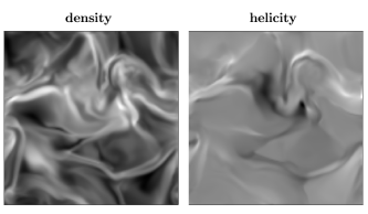
Figure 4: Density (left panel) and helicity (right panel) for the weak field model with $M_{A}=6.7$.

The density compressions in these models are associated with shock fronts. Helicity density can also increase across a shock. For example, consider a locally sheared, force free magnetic field of the form

$${\mbox{\boldmath$B$}}=B_{0}\left(\hat{x}\cos{k_{0}z}+\hat{y}\sin{k_{0}z}\right).$$ (15)

The vector potential is

$${\mbox{\boldmath$A$}}=-k_{0}^{-1}{\mbox{\boldmath$B$}},$$ (16)

so the helicity density is $-k_{0}^{-1}B_{0}^{2}$. Suppose the fluid is compressed in the $\hat{z}$ direction, so that the initial and final coordinates $z_{0}$ and $z$ are related by $z=\alpha z_{0}$, with $\alpha<1$. It can be shown from eqn. (6), or from intuitive arguments, that $B$ still has the form (15), but with $B_{0}\rightarrow\alpha^{-1}B_{0}$ and $k_{0}\rightarrow\alpha^{-1}k_{0}$. The helicity density then increases by a factor $\alpha^{-1}$, which is the same factor by which the mass density increases.

3 Parameter Space

The dimensionless parameters of astrophysical turbulence define the scope of the problem and should influence the choice of numerical technique. Here we define and give quantitative expressions for some important parameters.

3.1 Macroscopic Parameters

The ratio of gas pressure to magnetic pressure is usually denoted by $\beta\equiv 8\pi P/B^{2}$, which is closely related to the ratio of the sound speed $v_{S}$ to the Alfvén speed $v_{A}$; $v_{S}^{2}/v_{A}^{2}=\gamma\beta/2$, where $\gamma$ is the ratio of specific heats. If $\beta$ is either very small or very large, the acoustic and Alfvén frequencies are very different, with consequences for choice of simulation technique.

The ratios of the mean flow speed $v$ to $v_{S}$ and $v_{A}$, respectively, are denoted by the sonic and Alfvén Mach numbers $M$ and $M_{A}$. When $M\gg 1$, compressibility effects are important and the flow is pervaded by shocks, requiring an algorithm which treats them accurately.

The importance of self gravity is measured by the Jeans length $\lambda_{J}$. Turbulent pressure effectively increases $\lambda_{J}$. This is captured by a heuristic expression for $\lambda_{J}$ in a turbulent medium

$$\lambda_{J}\equiv\left[\frac{\pi v_{S}^{2}\left(1+M^{2}(\lambda_{J})\right)}{G\rho}\right]^{1/2},$$ (17)

where $M^{2}(\lambda_{J})$ is the Mach number of the turbulence at wavelengths less that $\lambda_{J}$; turbulence at longer wavelengths does not contribute to pressure support CHA1951 ; BFH1987 ; PUD1990 . Equation (17) reverts to the usual definition of the Jeans length as $M\rightarrow 0$. Truelove et al. TKM1997 have shown that unless the size of the grid, $\Delta x$, remains less than about $0.25$ of the local $\lambda_{J}$, the system is subject to spurious local fragmentation.

3.2 Microscopic Parameters

Complete expressions for plasma transport coefficients are given by BRA1965 . We are primarily concerned here with the magnetic and viscous diffusivities, which are conveniently given in terms of the electron and ion collision times $\tau_{e}$ and $\tau_{i}$

$$\tau_{e}=\frac{2.9\times 10^{-2}}{(\Lambda/10)}\frac{T^{3/2}}{n_{e}Z}s;\;\;\tau_{i}=\frac{1.7}{(\Lambda/10)}\frac{A^{1/2}T^{3/2}}{n_{e}Z^{3}}s.$$ (18)

In eqn. (18), $T$ is given in degrees K, $\Lambda$ is the Coulomb logarithm ($\Lambda=9.4-1.15\log{n_{e}}+3.45\log{T}$ for $T<5.8\times 10^{5}K$ and $\Lambda=15.9-1.15\log{n_{e}}+2.3\log{T}$ for $T>5.8\times 10^{5}K$), and $A$ and $Z$ are the ionic atomic number and charge, respectively. The electron density $n_{e}$ is expressed in cgs units; cm^-3.

The magnetic diffusivity $\lambda_{\Omega}$ introduced in eqn. (2) can also be expressed in terms of the electron skin depth $\delta_{e}\equiv c(m_{e}/4\pi n_{e}e^{2})^{1/2}$ = $5.4\times 10^{5}n_{e}^{-1/2}$cm and $\tau_{e}$ as

$$\lambda_{\Omega}=\frac{\delta_{e}^{2}}{\tau_{e}}=9.9\times 10^{12}\left(\Lambda/10\right)\frac{Z}{T^{3/2}}cm^{2}s^{-1}.$$ (19)

This numerical expression allows us to estimate the Lundquist number $S$

$$S\equiv\frac{L_{B}v_{A}}{\lambda_{\Omega}}=0.022\frac{L_{B}T^{3/2}B}{n_{e}^{1/2}(\Lambda/10)},$$ (20)

where the last expression holds in a hydrogen plasma. Under astrophysical conditions, $S$ is enormous: for example, in ionized interstellar gas with $T=10^{4}$, $n_{e}=1$, $B=3\times 10^{-6}G$, and $L_{B}=1$ pc, $S=10^{17}$. With the exception of extremely dense, cold environments such as protostellar disks, or systems with extremely small lengthscales, such as the outer layers of accreting neutron stars, $\lambda_{\Omega}$ is always much less than the numerical diffusivity arising from discretization.

The viscous diffusivity, or kinematic viscosity $\nu$, is

$$\nu=\frac{kT}{m_{i}}\tau_{i}=\frac{1.4\times 10^{8}}{(\Lambda/10)}\frac{T^{5/2}}{n_{e}A^{1/2}Z^{3}}cm^{2}s^{-1}.$$ (21)

The Reynolds number $R$ with respect to an organized flow $V$ on a lengthscale $L$ is defined as $LV/\nu$, and is almost always extremely large, confirming our expectation that astrophysical flow can be structured over a wide range of scales.

According to eqns. (19) and (21), the ratio of viscous to magnetic diffusivity, which is known as the magnetic Prandtl number $P_{r}$, is

$$P_{r}\equiv\frac{\nu}{\lambda_{\Omega}}=\frac{1.4\times 10^{-5}}{(\Lambda/10)^{2}}\frac{T^{4}}{n_{e}A^{1/2}Z^{4}}.$$ (22)

Typically, $P_{r}\gg 1$; in the example of fully ionized interstellar gas introduced above, $P_{r}=10^{11}$. Therefore, the kinetic energy spectrum should be truncated on much larger scales than the magnetic fluctuation spectrum KUA1992 ; MAC2002 ; CLV2002 The computations by Maron & Cowley MAC2002 show that the essentially constant shear of the velocity field on scales near the resistive scale generates tightly folded, or hairpin-like, magnetic structures.

If the ion cyclotron frequency $\omega_{ci}\sim 1.8\times 10^{4}BZ/A$ and the ion collision time $\tau_{i}$ satisfy the condition $\omega_{ci}\tau_{i}\gg 1$, the viscosity is highly anisotropic with respect to the magnetic field. The viscous force acting on shear flow parallel to the magnetic field is reduced by a factor of $(\omega_{ci}\tau_{i})^{2}$, while the parallel viscosity remains the same (see BRA1965 for a full description). Using eqn. (18), we see that $\omega_{ci}\tau_{i}$ is indeed large; in our numerical example, it is nearly 10⁵, implying very strong suppression of viscosity perpendicular to the magnetic field. Maron & Cowley MAC2002 have implemented the full tensor viscosity in their simulations of turbulent dynamos.

3.3 Implications for Numerical Techniques

In order for a numerical method to include diffusive processes, we would ideally require two things, namely (a) that it can resolve the physically important scales and (b) that it can handle the disparate time scales. Clearly, meeting each of these requirements alone is already a non-trivial task.

Resolving the physically interesting scales means separating the intrinsic numerical diffusion existing in any scheme from its physical counterpart. Simultaneously, it is desirable to cover scales much larger than the diffusive scales as well, in order to embed the problem in a realistic environment. Currently, studies are restricted to one of these regimes, for obvious reasons.

There are various ways to parametrize the small-scale physics in the large scale approach. Shock capturing is a familiar example (for a detailed discussion see e.g. LMD1998 ). Many finite-difference codes apply a von-Neumann-Richtmyer artificial viscosity NER1950 , spreading out the shock across several support points and not affecting the solution in smooth regions. Artificial viscosity mimicks physical viscosity in that it satisfies the Rankine-Hugoniot conditions, but on a much larger scale, which renders the numerical scheme very robust at low computational cost. It operates only where the flow is compressive.

Galsgaard & Nordlund GAN1995 implemented an artificial resistivity algorithm similar to artifical viscosity in their simulations of formation and dissipation of current sheets in the solar corona; see also Caunt & Korpi CAK2001 .

“Current sheet capturing” is intrinsically more complex than shock capturing. As we discuss in §4.3, the energy dissipated by a shock is independent of the magnitude of the diffusivity, but this does not hold for a current sheet. Moreover, the topological evolution of the magnetic field is determined primarily by processes in current sheets, and this imposes additional requirements on how they are treated. Detailed, small scale studies could be useful for developing a parameterization of the effects of diffusion on energy balance and topology. This is reminiscent of the approach taken in large eddy simulations, which numerically resolve the largest scales while treating the unresolved scales with a subgrid model (e.g. CAN1994 ; COO1999 ; ROC2001 ).

Godunov-type methods GOD1959 avoid broadening the shocks over many zones. They solve the Riemann problem defined by a set of advection equations for the physical variables and the physical states on both sides of the discontinuity. The upstream and downstream states are connected by a sequence of shocks or rarefaction waves, each of which satisfies the Rankine-Hugoniot conditions. As implementation of a full Riemann solver would involve determining the full wave structure and all wave propagation speeds, a variety of approximate Riemann solvers has been designed to simplify the process by disregarding certain wave types or linearizing the problem (see LMD1998 for details). Riemann solvers utilize the wave nature of hyperbolic equations, however, the diffusive terms are parabolic, so that they cannot be included in the Riemann solver directly.

An alternative approach has been taken in the so-called BGK-schemes BGK1954 , using the collisionless Boltzmann equation as a model of gas dynamics (see PRX1993 , and TAX2000 for MHD).

Needless to say, the $P_{r}\gg 1$ regime cannot be captured by numerical codes which solve the ideal fluid equations ($\eta=\nu=0$), since the numerical diffusivities for magnetic field and velocity are about the same size and occur at about the same scale, i.e. the grid scale. This is an argument for including viscosity and resistivity in the equations, in which case the physical diffusivities must be larger than their numerical counterparts, and their scales must be well separated. This is the approach taken by Maron & Cowley MAC2002 , who used a spectral code to study turbulence with widely separated, but resolved, viscous and resistive scales.

Several efforts have been made to connect the spatial scales by adaptive mesh refinement techniques BEO1984 ; BEC1989 for large eddy simulations COO1999 , general hyperbolic systems BER1998 , incompressible non-ideal MHD FGM1997 and for compressible MHD ZIE2001 ; BAL2001 . However, turbulent flows by definition connect scales over the whole domain, which complicates finding a suitable refinement criterion and may in the end yield only modest savings of time.

We have seen in §3.1 that timescales in astrophysical problems can differ by several orders of magnitude. Including diffusive processes aggravates the problem, as their time scales are generally orders of magnitude longer than the dynamical times. Any disparity in timescales leads to a stiff problem. Explicit methods – often the first choice because of their low time and memory needs – advance the solution by a time step $\Delta t$ which is given by the so-called Courant - Friedrichs - Levy (CFL) condition CFL1928

$$\Delta t\leq\frac{\Delta x}{c}$$ (23)

with the distance between two support points $\Delta x$ and a characteristic propagation speed $c$. Disparate characteristic speeds then lead to severe time step restrictions. Moreover, the slowly varying components may introduce numerical errors HUR2001 .

One solution to the problem is to choose a short timestep for the fast processes, and update the variables controlled by slow processes less frequently. Mac Low et al. MNK1995 used this so-called subcycling in their implementation of ambipolar diffusion in the ZEUS code. Depending on the problem, the critical processes often can be broken out and treated implicitly, while the remaining equations can be treated explicitly MAS1997 . Fully implicit schemes (e.g. JSE1997 ) can be unconditionally stable and independent of the time step chosen. Their main limitation lies in the tremendous computational needs in the multi-dimensional case. For a discussion of implicit methods and for a comparison between explicit and implicit shock capturing methods see HUR2001 ; YEE1997 . For a discussion of higher order finite difference schemes and their application to MHD turbulence simulations see BRA2001 .

As this brief discussion shows, a great variety of techniques can be brought to bear on MHD turbulence problems. Which technique is best depends very much on the problem at hand.

4 Results from Theories and Simulations

Theory offers an interpretive framework for simulations, while numerical experiments test turbulence theory, and can inspire new developments. Here, we discuss amplification of a field by turbulence in the context of dynamo theory, magnetic fluctuations, the formation of current sheets, and the dynamical effects of turbulence on large scales. The first three of these problems are closely related. The fourth is topical in view of recent simulations of star forming regions.

4.1 Turbulent Amplification of a Weak Field

Amplification of a weak magnetic field by turbulence is one of the main components of dynamo theory. A successful astrophysical dynamo theory must demonstrate that a dominant, large scale magnetic field can be generated by small scale turbulence, on a timescale which is virtually independent of the Lundquist number $S$ in the limit $S\rightarrow\infty$. This is a highly nonlinear problem, which involves multiple scales. It probably cannot be solved without numerical simulations, but in view of the extreme parameters involved it is unlikely to yield to brute force alone.

The growth rate of magnetic energy in a periodic domain is given by eqn. (12). Although the resistive term appears as a sink, some resistivity is necessary to effect irreversible topological change. Amplification occurs through work done by the flow. In general, there is also a surface integral $-c\int{\mbox{\boldmath$d$}}{\mbox{\boldmath$S$}}\cdot{\mbox{\boldmath$E$}}\times{\mbox{\boldmath$B$}}$ on the RHS of eqn. (12), which represents an energy flux through the boundaries.

Equation (12) says nothing about the structure of the field, and, in particular, whether magnetic energy is concentrated at large or small scales. If we formally set $\lambda_{\Omega}\equiv 0$, the ratio of fieldstrength to line length is preserved by incompressible motions. The only way to lengthen fieldlines in a finite volume is to wind or tangle them. Therefore, we expect that most of the energy will be in the rms field, rather than in the mean field. For example, if the protogalactic magnetic field were 10^-17 G GFZ2000 , the fieldlines would have been lengthened by more than a factor of 10¹¹ in the course of amplifying the field to its present strength. Yet, the large scale and small scale components of the galactic magnetic field are observed to be roughly equal ZWH1997 . It is not enough to argue that magnetic forces will prevent the field from becoming tangled on small scales. If the lines aren’t somehow lengthened, the field won’t be strengthened.

Of course, we are interested in $\lambda_{\Omega}\rightarrow 0$, not $\lambda_{\Omega}\equiv 0$. The fieldlines are allowed to break, and the question is whether they do so in a way which prevents power from piling up at the resistive scale and peaking instead at the large scale. Because $S$ is so large, topological constraints are strong, and we expect resistive boundary layers to form.

Let’s see how theories and simulations of dynamo theory address this problem. The most influential and detailed dynamo theory is the so-called mean field theory, which was proposed by Parker PAR1955 , and extended and formalized by Steenbeck, Krause & Rädler SKR1966 . Mean field theory is based on the idea that a large scale magnetic field $\langle{\mbox{\boldmath$B$}}\rangle$ can be generated from the average inductive electric field $\langle{\mbox{\boldmath$E$}}\rangle$ associated with small scale, helical velocity and magnetic fluctuations $\delta$$v$, $\delta$$B$. The dynamo property of small scale, helical fluctuations is known as the $\alpha$ effect. There is also diffusive transport of $\langle{\mbox{\boldmath$B$}}\rangle$, which is known as the $\beta$ effect. Although $\alpha$ and $\beta$ are in general tensors, it suffices for our purposes to write them as scalars. The induction equation for the mean field is

$$\frac{\partial\langle{\mbox{\boldmath$B$}}\rangle}{\partial t}=-c\mbox{\boldmath$\nabla$}\times\langle{\mbox{\boldmath$E$}}\rangle,$$ (24)

where

$$\langle c{\mbox{\boldmath$E$}}\rangle+\langle{\mbox{\boldmath$V$}}\rangle\times\langle{\mbox{\boldmath$B$}}\rangle=\lambda_{\Omega}\mbox{\boldmath$\nabla$}\times\langle{\mbox{\boldmath$B$}}\rangle-\langle\mbox{\boldmath$\delta$}{\mbox{\boldmath$v$}}\times\mbox{\boldmath$\delta$}{\mbox{\boldmath$B$}}\rangle\equiv\alpha\langle{\mbox{\boldmath$B$}}\rangle+\left(\lambda_{\Omega}+\beta\right)\mbox{\boldmath$\nabla$}\times\langle{\mbox{\boldmath$B$}}\rangle+....$$ (25)

In eqn. (25), $\langle{\mbox{\boldmath$V$}}\rangle$ is the large scale velocity field, and the “…” represent additional terms involving moments of the turbulent fluctuations and successively higher derivatives of $\langle{\mbox{\boldmath$B$}}\rangle$ (see Moffatt MOF1978 ). Note the correspondence between eqns. (24) and (25) and eqns. (1) and (2).

If $\alpha$ and $\beta$ are independent of $\langle{\mbox{\boldmath$B$}}\rangle$, eqn (24) is linear in $\langle{\mbox{\boldmath$B$}}\rangle$. Physically, this corresponds to neglecting the back reaction of the magnetic field on the turbulent velocity, so the linear case is sometimes called the kinematic case.

The linear version of eqn. (24) has solutions which vary exponentially in time. At large shear and low wavenumber $k$, the growth rate is approximately the geometric mean of the shear rate $V^{\prime}$ and the turbulent frequency $k\alpha$.

Standard mean field dynamo theory does not directly address the evolution of the small scale field, and the role of resistivity, on which the fate of the small scale field depends, is left somewhat implicit. Usually $\lambda_{\Omega}$ is dropped from eqn. (24), since $\beta$ is assumed to be much larger. A calculation by Moffatt MOF1978 of the $\alpha$ effect due to helical Alfvén waves demonstrates that $\alpha\equiv 0$ unless there is a phase difference between $\delta$$v$ and $\delta$$B$. In Moffatt’s model, the phase lag arises from magnetic diffusivity. At small $\lambda_{\Omega}$, $\alpha\propto\lambda_{\Omega}$, implying slow dynamo action at large $R_{m}$.

In more general calculations of $\alpha$, the diffusive damping time $(k^{2}\lambda_{\Omega})^{-1}$ is replaced by the correlation time $\tau$ of the turbulence. At large $R_{m}$, this is much shorter than the resistive time, and implies large growth rates for the dynamo. But $\beta$ does not distinguish between converting large scale field to small scale field and actually destroying field, so the behavior of the small scale fields are obscured by this treatment. Kulsrud & Anderson KUA1992 used the tools of mean field theory itself to follow the growth of the small scale field. They showed that at large $R_{m}$, the rms field $\langle B^{2}\rangle^{1/2}$ grows much faster than the mean field $\langle{\mbox{\boldmath$B$}}\rangle$, and is dominated by small scale fluctuations with a $k^{3/2}$ power spectrum.

A completely different perspective on kinematic dynamo theory emerges from solutions of the full magnetic induction equation for prescribed, chaotic flow. These studies, which are fully described up to 1995 in the volume by Childress & Gilbert CHG1995 , use a combination of numerical simulations at large $R_{m}$ and analytical theory to establish connections between the properties of the flow and the properties of the magnetic field. Although there are known examples of flows which amplify the magnetic field at a rate independent of $R_{m}$, as originally shown by Galloway & Proctor GAP1992 , the fields produced by these so-called fast dynamos are highly intermittent in space and fluctuate in sign, confirming at least qualitatively that small scale fields are dominant in kinematic dynamos at high $R_{m}$.

The kinematic theories are modified by dynamical effects. It was expected on general grounds that the dynamo would saturate as the magnetic field approached equipartition with the kinetic energy. A saturation process known as “Alfvénization” was first described by (Pouquet et al PFL1976 ). Saturation occurs because the small scale fluctuations increasingly resemble Alfvén waves as the mean field grows. In an ideal medium $\mbox{\boldmath$\delta$}{\mbox{\boldmath$B$}}\rightarrow\pm\mbox{\boldmath$\delta$}{\mbox{\boldmath$v$}}$ in Alfvén units, so their cross product also tends to zero, eliminating the $\alpha$ effect (also shown in the calculation by Moffatt). Alfvénization was first identified by Pouquet et al. PFL1976 using a spectral closure scheme, and later derived using quasilinear theory by Gruzinov & Diamond GRD1994 . In the model of Pouquet et al., kinetic helicity injected at the forcing scale generates magnetic helicity, which undergoes both a direct cascade, to high $k$, where it is resistively dissipated, and an inverse cascade, to low $k$. Alfvénization saturates the dynamo once the large scale field is roughly in equipartition with the kinetic energy. In the model of Gruzinov & Diamond, saturation by Alfvénization takes place when the ratio of kinetic to large scale magnetic energy is $\mathcal{O}(R_{m})$, confirming the dominance of small scale fields at large $R_{m}$. The difference between these calculations may lie in their treatments of diffusion. Gruzinov & Diamond explicitly include $\lambda_{\Omega}$, while Pouquet et al. took all the diffusivities to be eddy diffusivities, which are much larger than molecular diffusivities.

The role of kinetic helicity injection has been tested in simulations. Computations by Maron & Cowley MAC2002 , without kinetic helicity injection, show a peak in spectral power at the resistive scale, as predicted by Kulsrud & Anderson KUA1992 . Simulations by Maron & Blackman MAB2002 show that a large scale field is generated when kinetic helicity is injected, but that the growth rate is proportional to the resistive time. Nonlinear simulations with helical forcing by Brummell et al. BCT2001 show that the magnetic lengthscale is proportional to $R_{m}^{-1/2}$, while kinematic investigations testing the sensitivity of fast dynamo action to kinetic helicity have not found an inverse cascade  HCK1996 .

Thus, we see that much hinges on the resistive time, or, more broadly, the mechanism by which small scale fields are dissipated. Turbulent diffusion of $\langle{\mbox{\boldmath$B$}}\rangle$, parameterized by the $\beta$ effect, merely stands for spectral transfer out of the large scale. The possibility remains that turbulence could mix the field to the small scale, efficiently destroying it. However, numerical models by Cattaneo et al. CHK1996 , and subsequent analytical work by Kim K2000 suggest that the mixing is self limiting due to Lorentz forces.

The possibility that the small scale fields might escape through an open boundary rather than being destroyed in situ, leading to growth of the large scale field on the convective timescale rather than the resistive timescale, was raised by Parker PAR1992 and Blackman & Field BF2000 Up to now, neither analytical studies RK2000 nor numerical models BRD2001 have confirmed this idea.

Astrophysical dynamo theory is at a critical juncture. The fundamental premise of mean field dynamo theory - that kinetic helicity injected at small scales can drive the growth of a magnetic field at large scales - is supported by a variety of analytical treatments and numerical investigations. Mean field theory is a felicitous outcome of turbulence theory in the sense that it can be applied just by calculating a few parameters (or functions): $\alpha$, $\beta$, and the large scale shear. However, neither theory nor simulations have fully come to grips with the large value of $R_{m}$ and its implications for the small scale fields. From a numerical point of view, computations at large $R_{m}$ which can capture current sheets as well as accommodating a variety of boundary conditions would seem to be a prerequisite for either validating or superseding mean field theory.

4.2 Magnetic Fluctuations

Steady hydrodynamic turbulence, uninfluenced by boundaries, has been characterized in two regimes. Subsonic turbulence is incompressible, and follows the Kolmogorov scaling ($E(k)\propto k^{-5/3}$). Supersonic hydrodynamic turbulence is compressible, and better described as Burgers turbulence ($E(k)\propto k^{-2}$). (These power law spectra, and all subsequent ones, describe only the so-called inertial range, in which there is no driving or microscopic dissipation, only nonlinear spectral transfer.)

Both these limiting forms of turbulence are spatially intermittent in the sense that the variances of quantities such as the rate of energy dissipation undergo substantial fluctuations from point to point. In Burgers turbulence the basic structures are shock waves, and the large fluctuations and gradients occur principally in the shock fronts. In Kolmogorov turbulence, the basic units are eddies, and intermittency is represented by the concentration of vorticity into small structures. Intermittency does not affect the energy spectrum of Burgers turbulence (the Fourier spectrum of a shock itself is $k^{-2}$), but is thought to steepen the Kolmogorov spectrum. This occurs through the local enhancement of the dissipation rate at small scales LES1990 .

Hydrodynamic turbulence in unstratified, nonrotating systems is isotropic. A uniform component of magnetic field causes turbulence to be anisotropic.

An ideal, adiabatic fluid with a uniform component of magnetic field has three linear modes: the shear Alfvén mode, and the fast and slow magnetosonic modes. The velocity field $\delta$$v$ of the Alfvén mode, is solenoidal, and this mode is driven purely by magnetic tension. The dispersion relation is $\omega=k_{\parallel}v_{A}\equiv\omega_{A}$, where $k_{\parallel}$ is the component of $k$ parallel to the large scale magnetic field. The fast and slow magnetosonic modes are compressive, and driven by a combination of gas pressure, magnetic pressure, and magnetic tension.

Since the shear Alfvén mode is noncompressive, it is reasonable to ask whether a strong ($\beta<1$) magnetic field permits a regime of pure shear, supersonic turbulence. The answer is no.

First, suppose ${\mbox{\boldmath$k$}}_{\perp}\equiv 0$. Then, the nonlinear magnetic pressure gradient associated with the fluctuating transverse magnetic field drives a compressive parallel flow, causing an Alfvén wavetrain to steepen nonlinearly into a train of weak shocks COK1974 , much as a sound wave steepens. The only exception is the infinitely long, circularly polarized wave, which is an exact solution of the ideal MHD equations. The outcome of the evolution of an ensemble of parallel propagating Alfvén waves is a series of shocks, similar to Burgers turbulence, with $k^{-2}$ kinetic and magnetic energy spectra GAO1996 . The steepening time depends on amplitude as $(\delta v/v_{A})^{-2}$, while the steepening time of an acoustic wave is proportional to $(\delta v/v_{S})^{-1}$. In this sense, shear waves survive longer in a low $\beta$ plasma than compressive waves of the same amplitude, by a factor of order $\beta^{-1/2}(v_{A}/\delta v)$, but the outcome in either case is a compressive flow dominated by shocks, and the difference in timescales is only significant for small wave amplitude.

Although Burgers turbulence was originally based on 1D flow, 3D simulations of supersonic MHD turbulence show similar rapid evolution to a shock dominated flow. The distribution of shock strengths in simulations of driven and decaying turbulence, with and without magnetic fields, has been studied by Smith et al. SMZ2000 ; SMH2000 .

The steepening of Alfvén waves, which can be viewed as a cascade in $k_{\parallel}$, is suppressed if $\beta\geq 1$. Under the assumption of incompressibility, and in contrast to the highly compressible low $\beta$ case, interactions occur only between oppositely directed wave packets. In particular there is no self interaction of the kind which leads to steepening.

The incompressible shear Alfvén wave cascade is highly anisotropic, with power transferred much more rapidly in $k_{\perp}$ than in $k_{\parallel}$. In physical space, the correlation length transverse to the mean field is much shorter than the correlation length along it. These anisotropic states can be described by so-called reduced MHD S1976 , which is a quasi-2D approximation describing elongated magnetic structures. It is often applied to (and, indeed, was derived for), low $\beta$ plasmas, but it neglects the parallel steepening which leads to shocks. This, as we said above, is a good approximation for long parallel Alfvén transit times and small turbulent amplitudes.

There is not yet complete consensus on the cascade itself. Weak MHD turbulence, in which an individual Alfvén wave packet survives for many periods, can be viewed as weakly perturbative resonant interactions between multiple waves. Sridhar & Goldreich SRG1994 argued that the dominant interaction is a four wave interaction, which results in a spectrum $E(k)\propto k^{-7/3}$. Others NGB1996 ; BHN2001 ; GNN2002 claim that the dominant interactions are three wave interactions, and predict $E(k)\propto k^{-2}$.

In strong MHD turbulence, wave packets survive for only about one wave period. Goldreich & Sridhar GOS1995 developed the concept of a critically balanced cascade in which the wave frequency $\omega_{A}$ is the same as the nonlinear frequency $k_{\perp}v_{\perp}$. This, together with the requirement of constant spectral energy flux argument $k_{\perp}v_{\perp}^{3}$, leads to a Kolmogorov spectrum $E(k)\propto k^{-5/3}$ and wavenumber anisotropy $k_{\parallel}/k_{\perp}\propto k_{\perp}^{-1/3}$. Other theories of strong MHD turbulence predict $E(k)\propto k^{-3/2}$, including the original isotropic Iroshnikov-Kraichnan theory NAK2001 .

Numerical simulations, if free of confounding computational effects, could play a role in resolving these disagreements. Biskamp & Müller BIM2000 and Cho & Vishniac CHV2000 find $E(k)\propto k^{-5/3}$ over about one decade in $k$ space. Maron & Goldreich MAG2001 slightly extended the inertial range and found $E(k)\propto k^{-3/2}$. These authors argue that the spectrum is flattened because of intermittency. The crucial difference between the HD and MHD cases is that energy cascades in MHD only when oppositely directed wave packets collide; the small filling factor associated with intermittency reduces the collision rate, more than offsetting the enhanced dissipation associated with small structures.

Larger computations, with an extended inertial range, should shortly become available. The differences in the spectra obtained with different codes and under different forms of driving (Biskamp & Müller studied decaying or isotropically forced turbulence, Cho & Vishniac studied isotropically forced turbulence, and Maron & Goldreich studied anisotropically forced turbulence) are at this point comparable to the theoretical disagreements. A joint exercise in which different groups simulated identical problems and implemented identical diagnostics might be quite enlightening.

A variety of processes can terminate the cascade at short wavelengths (see LIG2001 for a recent discussion). These include fluid effects, such as ion-neutral friction, and kinetic effects such as ion gyroresonance absorption and electron Landau damping QG1999 . The extension of the magnetic spectrum to scales below the viscous cutoff in a high Prandtl number plasma is discussed by MAC2002 and CLV2002 .

4.3 Intermittency: Current Sheets and Flux Tubes

Simulations of MHD turbulence show strong intermittency in the distribution of magnetic field gradients, or current. In the weak field, high Prandtl number simulations of MAC2002 , the fluctuating field is tightly folded. These results suggest that we look at current sheets.

Current sheets and filaments are sites of intense local heating, and possibly particle acceleration, which makes them interesting in their own right. It is quite likely that in most astrophysical systems, significant departures from flux freezing occur only in these regions, so their existence is important in the evolution of magnetic field topology, and for dynamo action, (see §4.1). Reconnection at magnetic X-points drives strong, small scale jets. Simulations by Galsgaard & Nordlund GAN1996 show highly time variable dissipation rates associated with the formation and disruption of large scale current sheets.

Current sheets are a prerequisite of, and accompany, magnetic reconnection. Reconnection is a resistive process which occurs on a timescale intermediate between the Ohmic time and the Alfvén time. The reconnection time $\tau_{rec}$ is often parameterized by the Lundquist number $S$; $\tau_{rec}$ scales as $S^{p}$ with $0\leq p<1$. If $p=0$, the reconnection is said to be fast (in correspondence with the definition of a fast dynamo). In Sweet-Parker reconnection, $p=1/2$ P1979 , and resistive tearing modes in slabs and cylinders have $p=3/5$, and $p=1/3$, respectively B1978 . The formation and behavior of current sheets has been studied for many years. Most of this work has focussed on plasmas in or near magnetostatic equilibrium, which can be expected if $\beta\ll 1$ and the plasma is either allowed to relax or is driven at frequencies far below its characteristic Alfvén frequency. Such conditions hold, for example, in stellar coronae, in which the magnetic fieldlines are tied to the underlying photosphere, and evolve quasistatically in response to slow photospheric motion.

Current sheets form as a plasma seeks equilibrium while obeying the topological constraints imposed by flux freezing M1985 . Topological constraints can arise from features such as null points S1971 or separatrices LOW1988 ; ZP1990 ; LC1996 . Sweet  S1958 and Parker  P1972 suggested that shearing and winding the footpoints of an initially uniform field will create current sheets. Even a simple sinusoidal deformation of the boundaries of a sheared magnetic slab can induce the formation of a current sheet HK1985 .

As a simple example of how current sheets can form, consider the magnetic field of a pair of neighboring, uniformly magnetized superconducting spheres, with antiparallel magnetic dipole moments, surrounded by a perfectly conducting, zero pressure plasma. Some fieldlines have both endpoints on the same sphere, and others have one endpoint on each sphere.

Now suppose that one sphere rotates on its magnetic axis by an angle $\phi$. The fieldlines which are not connected to the other sphere also rotate by $\phi$, but the fieldlines which are connected to the other sphere cannot rotate uniformly because one endpoint remains fixed. The separatrix surface which divides the two domains of magnetic connectivity becomes a current sheet: the field outside it is sheared while the field inside it is not.

There is still no comprehensive theory for exactly when current sheets form, and how their properties reflect the underlying magnetic topology. Nevertheless, analytical arguments V1985 ; LOS1994 and numerical experiments MSV1989 ; LOS1994 ; GAN1995 show that shear, or equivalently current density, grows exponentially rapidly in line tied magnetic fields with randomly moving footpoints. This has some of the same consequences as an exact singularity, which cannot form in any case in even a slightly resistive plasma.

These results are not fully applicable to MHD turbulence, in which the magnetic field is not in equilibrium. Nevertheless, current sheets form in flows with magnetic null points P1987 . The underlying mechanism for the growth of the current is the random stretching of neighboring fieldlines, which leads to large cross-field shear.

What are the consequences of current sheet formation for dissipation of magnetic energy? That is, if energy per unit volume $\dot{e}$ is being added to a system by a driving process, under what circumstances can this energy can be dissipated in current sheets?

Consider a current sheet of area $L^{2}$ and width $\delta$. Assume the current sheet structure is given by the Sweet-Parker theory, so that $\delta=LS^{-1/2}=(L\lambda_{\Omega}/v_{A})^{1/2}$. If $N(L)dL$ is the number density of current sheets with $L$ between $L$ and $L+dL$, then the rate at which energy is dissipated by current sheets in this size range is

$$d\dot{w}=\frac{B^{2}}{4\pi}\frac{v_{A}}{L}N(L)L^{2}\delta dL=\frac{B^{2}}{4\pi}N(L)\left(L^{3}\lambda_{\Omega}v_{A}\right)^{1/2}dL.$$ (26)

The rate of energy dissipation by all current sheets is obtained by integrating eqn. (26) over $L$:

$$\dot{w}=\frac{B^{2}}{4\pi}\left(\lambda_{\Omega}v_{A}\right)^{1/2}\int dLN(L)L^{3/2}.$$ (27)

If $\dot{e}$ is independent of $\lambda_{\Omega}$ as $\lambda_{\Omega}\rightarrow 0$, then $\int dLN(L)L^{3/2}$ must scale as $\lambda_{\Omega}^{-1/2}$ in this limit. This would imply an unbounded number of current sheets as $\lambda_{\Omega}\rightarrow 0$, which is virtually equivalent to a pileup of magnetic energy in fluctuations at the resistive scale.

There are alternative possibilities. One is that the current sheets are not structured according to the Sweet-Parker picture. If $\delta$ scaled as $\lambda_{\Omega}$, as it does (up to a logarithmic factor) in Petschek’s model of fast reconnection (reviewed in P1979 ), then $\int dLN(L)L^{3/2}$ could be independent of $\lambda_{\Omega}$. Note, however, that while in the Sweet-Parker theory, magnetic energy is converted to kinetic energy and to heat at about the same rate, in Petschek’s theory magnetic energy is converted predominantly to kinetic energy, and that the realizability of Petschek’s model has recently been questioned B1993 ; UZK2000 .

The second possibility is that the magnetic and velocity fields adjust themselves such that the driving just balances the damping, as they do in mechanical systems such as linear harmonic oscillators. Thus, the energy input rate $\dot{e}$ would depend on $\lambda_{\Omega}$, while the applied force itself, presumably would not.

Dedicated simulations of current sheets and reconnection regions themselves allow us to study the small scale aspects of the problem. It is equally important to understand how current sheets are embedded in the overall flow. This has already been done to some extent for laboratory experiments UZK2000 . Ultimately, it may be possible to parameterize magnetic reconnection in simulations on larger scales.

Finally, we mention an even more extreme form of intermittency: the segregation of the magnetic field into thin tubes. This is observed in the solar photosphere, where magnetic flux tubes, or sheets, just a few hundred km thick are seen at the borders of convective cells. Flux tubes can form only in high $\beta$ plasma, so that gas pressure can balance magnetic pressure at the tube walls.

Early attempts to explain photospheric flux tubes relied on a two stage process, proposed by Parker, for concentrating a diffuse field into organized structures. According to this scenario, thermal convection would sweep the field to the borders of convective cells, concentrating the field up to equipartition with the flow. Then reduced convective heat transport would cool the gas, “collapsing” the tube and bringing it to equipartition with the thermal plasma.

An alternative possibility is that intermittent fields are generated in situ. It has been shown that small scale turbulent thermal convection operates as a dynamo, and generates a magnetic field with a broad tail of high energy features CAT1999 .

It is unclear whether a dynamo operating in a high $\beta$ plasma should always produce flux tubes. In the solar case, the turbulence is organized by stratification and the thermal gradient, and is subsonic. If the turbulence were supersonic and the field were amplified to equipartition, then flux tubes could not persist.

4.4 Dynamical Effects of Turbulence

The stresses associated with turbulence can exert dynamical forces. In MHD turbulence, these forces include both magnetic stresses and the Reynolds stress. Observations suggest that these stresses are important in the interstellar medium, and especially in molecular clouds.

It was realized early that supersonic motions are nearly ubiquitous in molecular gas, and pose a problem. If the motions are associated with gravitational collapse, the implied star formation rate would be very high ZUE1974 , but if the motions are turbulent, they should be dissipated very quickly GOK1974 . This conundrum, together with the expectation that reasonably strong magnetic fields should be present, prompted analytical studies of Alfvénic turbulence under molecular cloud conditions ARM1975 ; ZWJ1983 ; E1985 . This work demonstrated that even when $M_{A}\ll M$ and the waves are purely transverse, ion-neutral friction and nonlinear steepening are strong damping mechanisms, which limit the lifetimes of Alfvén waves to a few 10⁶ yr or less under molecular cloud conditions.

Even so, under the assumption that the waves might be replenished by some energy source, various aspects of the theory of self gravitating clouds supported by Alfvén wave stresses were developed and applied to model clouds PUD1990 ; FAA1993 ; MCZ1995 ; MHP1997 ; MCH1999 . According to this theory, which is based on the the weak turbulence approach pioneered by Dewar DEW1970 , Alfvén waves have an isotropic stress tensor ${\mbox{\boldmath$P$}}=P_{w}{\mbox{\boldmath$I$}}$. The waves pressure - density relation is $P_{w}\propto\rho^{1/2}$ in a stratified, static medium, while $P_{w}\propto\rho^{3/2}$ under slow, spatially uniform changes in density with time. The negative polytropic index ($n=-1/2$) of the $P-\rho$ relation leads to a large center to surface pressure contrast, in accord with observations (see MCH1999 for a good discussion).

The theory of wave supported clouds is most relevant to objects which are slightly magnetically supercritical, that is, the ratio of mass to magnetic flux is slightly too large for magnetostatic support. If the clouds were subcritical they would be supported by the DC magnetic field. If they were highly supercritical, the amplitude of the turbulence required to sustain them would be so large that the weak turbulence theory would probably not apply, although they could still be turbulently supported. ¿From an observational viewpoint, the most likely candidates for wave support are dense cores with sonic or mildly supersonic linewidths MF1992 .

The picture of strongly supersonic turbulence which emerges from numerical simulations of molecular clouds is quite different from this analytical picture, primarily because, as we discussed in §4.2, generation of compressive disturbances is entirely unavoidable. These compressive disturbances, or shocks, sweep up most of the mass into thin layers in which the local Jeans length is small. These layers, and the even denser structures formed where layers intersect, collapse if the domain is magnetically supercritical, whether the turbulence is freely decaying or maintained in a steady state by driving HMK2001 ; OSG2001 . The driven models are globally stable in the sense that $\lambda_{J}$ computed using the total turbulent energy and mean density is larger than the length of the domain. The small, high density structures collapse because the turbulent power at wavelengths less than the local Jeans length is relatively small (see eqn. (17)), and because the intensity of turbulence inside the cores is comparable with the density outside. Nevertheless, the bound structures are small, and the role of numerical diffusion within them, which damps the turbulence and removes the support by the DC magnetic field, has not been quantified. Therefore, while the formation of turbulently supported clumps has not been found in the numerical models, their existence cannot be ruled out based on the present models.

5 Ambipolar Drift

As we have discussed in the preceding sections, both theoretical and computational aspects of astrophysical magnetohydrodynamics are dogged persistently by the enormous value of $R_{m}$. There is one situation, however, in which the magnetic diffusivity is large whether or not it is enhanced by turbulence: in weakly ionized gas, the magnetic field and plasma drift with respect to the neutrals. This so-called ambipolar drift is not entirely equivalent to resistive diffusion, because it preserves magnetic topology (the field is frozen to the plasma), but it does change the ratio of magnetic flux to mass, as originally pointed out in MS1956 , and dissipates fluctuations on small scales.

Full treatment of ambipolar drift requires solving the equations of MHD for the plasma and neutrals treated as distinct species coupled by collisions, ionization, and recombination DRA1986 . At the low ionization fractions expected in molecular clouds, the ion Alfvén speed $v_{Ai}\equiv B/\sqrt{4\pi\rho_{i}}$ can be several orders of magnitude larger than the other characteristic speeds in the problem, reducing the maximum possible timestep by a similar factor. This and other numerical issues related to implementation of ambipolar drift are discussed by MNK1995 ; TOT1995 ; MAS1997 ; STO1997 .

On timescales longer than the ion - neutral collision time $\tau_{in}$, and at low ionized mass fractions, the ion-neutral drift $v_{D}$ is determined by balancing the Lorentz force on the ions against the frictional drag by neutrals

$${\mbox{\boldmath$v$}}_{D}=\frac{\left(\mbox{\boldmath$\nabla$}\times{\mbox{\boldmath$B$}}\right)\times{\mbox{\boldmath$B$}}}{4\pi\rho_{i}\nu_{in}}\equiv\frac{v_{Ai}^{2}\tau_{in}}{L_{B}}\hat{f},$$ (28)

where $\hat{f}$ is a unit vector in the direction of the Lorentz force. The second equality in eqn. (28) can be taken as a definition of the magnetic lengthscale $L_{B}$. The quantity $v_{Ai}^{2}\tau_{in}$ has units of diffusivity, and from now on we refer to it as $\lambda_{AD}$. With this definition, $v_{D}=\lambda_{AD}/L_{B}$. Note that $\rho_{i}/\tau_{in}=\rho_{n}/\tau_{ni}$ and $\rho_{n}\approx\rho$, so $v_{Ai}^{2}\tau_{in}=v_{A}^{2}\tau_{ni}$, and $\lambda_{AD}$ is often expressed in the latter terms.

The ambipolar Reynolds number $R_{AD}$ is defined as the ratio of the bulk velocity $v$ to the drift velocity $v_{D}$

$$R_{AD}\equiv\frac{L_{B}v}{\lambda_{AD}},$$ (29)

and measures how well the magnetic field is frozen to the bulk fluid on scale $L_{B}$ ZWB1997 . Setting $R_{AD}=1$ correctly predicts the thickness of shocks in which the main dissipation mechanism is ion-neutral friction DRM1993 , the wavelength at which Alfvén waves are critically damped KUP1969 , and the minimum size of an eddy which can wind up a magnetic field ZWB1997 .

Simulations of supersonic MHD turbulence PZN2000 with varying strengths of ambipolar drift shows that, on average, the drift smooths out the current, and reduces the rms Lorentz force.

We expect (with one caveat discussed at the end of this section) that the magnetic field should show very little structure below the scale $L_{min}\equiv\lambda_{AD}/v$ at which $R_{AD}=1$. Consider a volume $L^{3}$ of turbulent gas with mean density $\rho$, turbulent velocity $v$, and mean magnetic field $B$. If we introduce the crossing time $\tau_{d}\equiv L/v$ and the Alfvén Mach number $M_{A}\equiv v/v_{A}$, then we can write

$$\frac{L_{min}}{L}=\frac{1}{M_{A}^{2}}\frac{\tau_{ni}}{\tau_{d}}.$$ (30)

Expressing $v$ in units of km s^-1 as $v_{5}$, and $L$ in pc as $L_{pc}$, $\tau_{d}\sim 3\times 10^{13}L_{pc}/v_{5}$ s. For the particle species expected in molecular clouds, $\tau_{ni}\sim 5\times 10^{8}n_{i}^{-1}$s. With the ionization equilibrium relation $n_{i}\sim 10^{-5}n_{n}^{1/2}$ (cgs; MZG1993 ), eqn. (30) becomes

$$\frac{L_{min}}{L}=1.7\frac{v_{5}}{n^{1/2}L_{pc}}\frac{1}{M_{A}^{2}}.$$ (31)

Comparing eqn. (31) with the grid spacing $\Delta x/L=1/N$, we see that a moderately large numerical simulation (say 256³), which is not highly super-Alfvénic or extremely dense, should resolve almost all the magnetic structure associated with turbulence.

Equation (30) can also be written in terms of the critical magnetic field $B_{c}\equiv 2\pi G^{1/2}\rho L$ and the free fall time $\tau_{ff}\equiv(4\pi G\rho)^{-1/2}\sim 5.5\times 10^{14}n_{n}^{-1/2}$s as

$$\frac{L_{min}}{L}=\left(\frac{B}{B_{c}}\right)^{2}\frac{\tau_{ni}\tau_{d}}{4\tau_{ff}^{2}}\sim\left(\frac{B}{B_{c}}\right)^{2}\frac{\tau_{ni}}{4\tau_{ff}},$$ (32)

where the last step holds for virial equilibrium; $\tau_{ff}\sim\tau_{d}$. Of course, eqn. (30) is entirely independent of $G$.

The modest value of $R_{AD}$ in molecular clouds has been commented upon and exploited by KHM2000 ; OSM2002 .

Ambipolar drift is essentially diffusive when the magnetic field has a well ordered, well combed structure. Because the ambipolar diffusivity is proportional to $B^{2}$, the diffusion is nonlinear. Sharp fronts can be generated in the vicinity of magnetic nulls, and minima are steepened BRZ1994 ; MNK1995 ; ZWB1997 ; MAS1997 .

6 Summary and Future Agenda

The theme of this paper is how numerical simulations can best cope with the enormous magnetic Reynolds numbers encountered in most astrophysical problems. We argued that, because $R_{m}$ (and the Lundquist number $S$) are so large, resistive effects occur primarily in thin sheets or filaments, which must be treated accurately in order to follow the topological evolution of the magnetic field.

In §2, we reviewed the magnetic induction equation, giving the solution in the ideal limit, and derived equations for magnetic helicity and magnetic energy. We tested helicity conservation in the ZEUS code by simulating the evolution of the ideal kink mode, and studied fluctuations of helicity in a simulation of a turbulent cloud. The first of these problems is especially suitable for benchmarking numerical codes. That is, it yields a quantitative estimate of the numerical resistivity in the code, from which one can compute the resistive timescale (at least in smooth regions, on large scales) and assess whether it is much longer than other timescales of interest. One can also compare the performance of different codes.

In §3, we discussed some important dimensionless parameters in astrophysical MHD problems. We verified the large size of the Lundquist number $S$ and magnetic Reynolds number $R_{m}$ under most conditions, and showed that the magnetic Prandtl number, the ratio of viscous to magnetic diffusivity, is also usually large. This implies that magnetic structure will generally extend to smaller scales than velocity structure. We briefly summarized a variety of numerical techniques from the perspective of the large $S$ limit.

In §4, we discussed theoretical and numerical results on several basic problems. In §4.1 we discussed the amplification of magnetic fields by turbulence, and argued that the successful operation of a large scale dynamo depends on fast diffusion of the magnetic field. In §4.2 we discussed MHD turbulence itself. In §4.3 we discussed current sheets, which may provide the fast diffusion necessary for a dynamo, and may be produced in turbulence as a form of intermittency. In §4.4, we discussed the dynamical effects of turbulence, and its importance in molecular clouds.

In §5, we discussed ambipolar drift as a mechanism for increasing the magnetic diffusivity in low density, weakly ionized gas. It is now possible to simulate turbulent molecular clouds at a resolution which accounts for all magnetic structure down to the ambipolar diffusion scale. Under certain conditions, however, ambipolar drift can mediate the formation of current sheets, possibly leading to rapid magnetic reconnection.

It is fortunate that a number of different groups are simulating MHD turbulence under astrophysical conditions, using a variety of codes and techniques. There is substantial agreement on a number of issues, such as the short decay time of supersonic turbulence, but disagreement on others, such as the spectrum of strong MHD turbulence. A dedicated effort at benchmarking, in which different groups simulated identical problems and implemented identical diagnostics, would provide some perspective. We suggested in §4.2 that such an exercise be carried out for strong MHD turbulence.

It is unlikely that it will ever be possible to adequately resolve current sheets and global dynamics in a single simulation. Local studies of current sheets and magnetic reconnection are essential in capturing the physics of these layers. It is equally important to understand how they are embedded in the overall flow, as this constrains their properties, sets the boundary conditions for reconnection, and is necessary for understanding how to parameterize the effects of current sheets in global simulations. The inability to deal adequately with this small scale structure is the greatest present challenge to understanding magnetic field evolution in turbulent flows.

Acknowledgements: We are grateful to E. Falgarone and T. Passot for organizing the conference, and for their hospitality. Our discussions with A. Burkert, M.-M. Mac Low, and J. Maron were especially useful, as were L. Mestel’s comments on the manuscript. FH gratefully acknowledges support by the Feodor-Lynen program of the Alexander von Humboldt Foundation. The (U.S.) National Science Foundation provided partial support through grants AST-9800616 and AST-0098701 to the University of Colorado, and through support to the National Center for Atmospheric Research.

References

- (1) J. Arons, C.E. Max: ApJL 196, 77 (1975)
- (2) D.S. Balsara: J. Comp. Phys. 174, 614 (2001)
- (3) G. Bateman: MHD Instabilities, MIT Press (1978)
- (4) M.J. Berger, P. Colella: J. Comp. Phys. 82, 64 (1989)
- (5) M.J. Berger, J. Oliger: J. Comp. Phys. 53, 484 (1984)
- (6) M.J. Berger, R. J. LeVeque: SIAM J. Numer. Anal. 35, 2298 (1998)
- (7) P.L. Bhatnagar, E. P. Gross, M. Krook: Phys. Rev. 94, 511 (1954)
- (8) A. Bhattacharjee, C.S. Ng: ApJ 548, 318 (2001)
- (9) D. Biskamp: Nonlinear Magnetohydrodynamics, Cambridge Univ. Press (1993)
- (10) D. Biskamp, W.-C. Müller: Physics of Plasmas 7, 4889 (2000)
- (11) E. Blackman, G.B. Field: ApJ 534, 984 (2000)
- (12) S. Bonazzola, E. Falgarone, J. Heyvaerts, M. Perault, J.L. Puget: A&A 172, 293 (1987)
- (13) S.I. Braginski: Rev. Plasma Phys. 1 205 (1965)
- (14) A. Brandenburg: ’Computational aspects of astrophysical MHD and turbulence’ in The Fluid Mechanics of Astrophysics and Geophysics, vol 8. ed. A. Ferriz-Mas, astroph/0109497
- (15) A. Brandenburg, W. Dobler: A&A 369, 329 (2001)
- (16) A. Brandenburg, E.G. Zweibel: ApJL 427, 91 (1994)
- (17) N.H. Brummell, F. Cattaneo, S.M. Tobias: Fl. Dyn. Res. 28, 237 (2001)
- (18) V.M. Canuto: ApJ 428, 729 (1994)
- (19) F. Cattaneo: ApJL 515, 39 (1999)
- (20) F. Cattaneo, D.W. Hughes, E.-J. Kim: Phys. Rev. Lett. 76, 2057 (1996)
- (21) S.E. Caunt, M.J. Korpi: A&A 369, 706 (2001)
- (22) S. Chandrasekhar: Proc. R. Soc. London A 210, 26 (1951)
- (23) S. Childress, A.D. Gilbert: Stretch, Twist, Fold: The Fast Dynamo, (Springer Heidelberg 1995)
- (24) J. Cho, A. Lazarian, E. Vishniac: ApJL submitted (2002)
- (25) J. Cho, E. Vishniac: ApJ 539, 273 (2000)
- (26) R.H. Cohen, R.M. Kulsrud: ’Nonlinear hydromagnetic wave evolution in the solar wind’ in Solar wind three; Proceedings of the Third Conference, Pacific Grove, Calif., March 25-29, 1974, p. 382
- (27) A.W. Cook: J. Comp. Phys. 154, 117 (1999)
- (28) R. Courant, K.O. Friedrichs, H. Lewy: Über die partiellen Differenzengleichungen der mathematischen Physik. Math. Ann. 100, 32 (1928)
- (29) R.L. Dewar: Phys. Fluids 13, 2710 (1970)
- (30) B.T. Draine: MNRAS 220, 133 (1986)
- (31) B.T. Draine, C.F. McKee: ARA&A 31, 373 (1993)
- (32) B.G. Elmegreen: ApJ 299, 196 (1985)
- (33) M. Fatuzzo, F.C. Adams: ApJ 412, 146 (1993)
- (34) H. Friedel, R. Grauer, C. Marliani: J. Comp. Phys. 134, 190 (1997)
- (35) D.J. Galloway, M.R.E. Proctor: Nature 356, 691 (1992)
- (36) K. Galsgaard, Å. Nordlund: unpublished Technical Report of the University of Copenhagen (1995)
- (37) K. Galsgaard, Å. Nordlund: J. Geophys. Res. 101 13445 (1996)
- (38) S. Galtier, S.V. Nazarenko, A.C. Newell, A. Pouquet: ApJL 564, 49 (2002)
- (39) C.F. Gammie, E.C. Ostriker: ApJ 466, 814 (1996)
- (40) N.Y. Gnedin, A. Ferrara, E.G. Zweibel: ApJ 539, 505 (2000)
- (41) S. K. Godunov: Mat. Sb. 47, 271 (1959)
- (42) P. Goldreich, J. Kwan: ApJ 189, 441 (1974)
- (43) P. Goldreich, S. Sridhar: ApJ 438, 763 (1995)
- (44) A.V. Gruzinov, P.H. Diamond: Phys. Rev. Lett. 72, 1651 (1994)
- (45) T.S. Hahm, R. Kulsrud: Phys. Fluids 28, 2412
- (46) J.F. Hawley, J.M. Stone: Comp. Phys. Comm. 89, 1 (1995)
- (47) F. Heitsch, M.-M. Mac Low, R.S. Klessen: ApJ 547, 280 (2001)
- (48) F. Heitsch, E.G. Zweibel, M.-M. Mac Low, P.S. Li, M.L. Norman: ApJ 561, 800 (2001)
- (49) D.W. Hughes, F. Cattaneo, E. Kim: Phys. Lett. A 223, 167 (1996)
- (50) A. Hujeirat, R. Rannacher: New Astr. Rev. 45, 425 (2001)
- (51) O.S. Jones, U. Shumlak, D.S. Eberhardt: J. Comp. Phys. 130, 231 (1997)
- (52) E. Kim: Phys. Plasmas 7, 1746 (2000)
- (53) R.M. Kinney, B. Chandran, S. Cowley, J.C. McWilliams: ApJ 545, 907 (2000)
- (54) R.S. Klessen, F. Heitsch, M.-M. Mac Low: ApJ 535, 887 (2000)
- (55) R.M. Kulsrud, S. W. Anderson: ApJ 396, 606 (1992)
- (56) R.M. Kulsrud, W.P. Pearce: ApJ 156, 445 (1969)
- (57) M. Lesieur: Turbulence in Fluids (Kluver, Dordrecht 1990)
- (58) R.J. LeVeque, D. Mihalas, E. Dorfi, E. Müller: “Computational Methods for Astrophysical Fluid Flow” in 27th Saas-Fee Advanced Course Lecture Notes, eds. O. Steiner and A. Gautschy (Springer 1998)
- (59) Y. Lithwick, P. Goldreich: ApJ 562, 279 (2001)
- (60) D.W. Longcope, S.C. Cowley: Phys. Plasmas 3, 2885 (1996)
- (61) D.W. Longcope, H.R. Strauss: ApJ 437, 851
- (62) B.C. Low, R. Wolfson: ApJ 324, 574 (1988)
- (63) M.-M. Mac Low, M.L. Norman, A. Königl, M. Wardl: ApJ 442, 726 (1995)
- (64) M.-M. Mac Low, M.D. Smith: ApJ 491, 596 (1997)
- (65) J. Maron, E.G. Blackman: Phys. Rev. Lett. submitted, astroph/0110018
- (66) J. Maron, S. Cowley: (astro-ph/0111008)
- (67) J. Maron, P. Goldreich: ApJ 554, 1175 (2001)
- (68) C.E. Martin, J. Heyvaerts, E.R. Priest: A&A 326, 1176 (1997)
- (69) C.F. McKee, E.G. Zweibel: ApJ 440, 686 (1995)
- (70) C.F. McKee, J.H. Holliman II: ApJ 522, 313 (1999)
- (71) C.F. McKee, E.G. Zweibel, A.A. Goodman, C. Heiles: ’Magnetic Fields in Star-Forming Regions – Theory’ in Protostars and Planets III, eds: E.H. Levy, J.I. Lunine (University of Arizona Press 1993), p. 327
- (72) L. Mestel & L. Spitzer: MNRAS 116, 503 (1956)
- (73) Z. Mikić, D.D. Schnack, G. van Hoven: ApJ 338, 1148 (1989)
- (74) H.K Moffatt: Magnetic field generation in electrically conducting fluids, Cambridge University Press (1978)
- (75) H.K. Moffatt: J. Fl. Mech 159, 359 (1985)
- (76) P.C. Myers, G.A. Fuller: ApJ 396, 631 (1992)
- (77) K. Nakayama: ApJ 556, 1027 (2001)
- (78) J. von Neumann, R.D. Richtmyer: J. Appl. Phys. 23, 232 (1950)
- (79) C.S. Ng, A. Bhattacharjee: ApJ 465, 845 (1996)
- (80) V. Ossenkopf, M.-M. Mac Low: in preparation
- (81) E.C. Ostriker, J.M. Stone, C.F. Gammie: ApJ 546, 980 (2001)
- (82) P. Padoan, E.G. Zweibel, Å. Nordlund: ApJ 540, 332 (2000)
- (83) E.N. Parker: ApJ 122, 293 (1955)
- (84) E.N. Parker: ApJ 174, 499 (1972)
- (85) E.N. Parker: Cosmical Magnetic Fields, Oxford Univ. Press (1979)
- (86) E.N. Parker: ApJ 401, 137 (1992)
- (87) A. Pouquet: in Astrophysical Fluid Dynamics,eds. J.-P. Zahn & J. Zinn-Justin, Elsevier (1993)
- (88) A. Pouquet, U. Frisch, J Leorat: J. Fluid Mech. 77, 321 (1976)
- (89) K.H. Prendergast, K. Xu: J. Comp. Phys. 109, 53 (1993)
- (90) R.E. Pudritz: ApJ 350, 195 (1990)
- (91) E. Quataert, A. Gruzinov: ApJ 520, 248 (1999)
- (92) R.R. Rafikov, R.M. Kulsrud: MNRAS 314, 839 (2000)
- (93) F. J. Robinson, K.L. Chan: MNRAS 321, 723
- (94) M.D. Smith, M.-M. Mac Low, F. Heitsch: A&A 362, 333 (2000)
- (95) M.D. Smith, M.-M. Mac Low, J.M. Zuev: A&A 356, 287 (2000)
- (96) S. Sridhar, P. Goldreich: ApJ 432, 612 (1994)
- (97) M. Steenbeck, F. Krause, K.H. Rädler: Z. Naturforsch. A 21, 369 (1966)
- (98) J.M. Stone: ApJ 487 271 (1997)
- (99) J.M. Stone, M.L. Norman: ApJS 80, 753 (1992a)
- (100) J.M. Stone, M.L. Norman: ApJS 80, 791 (1992b)
- (101) H.R. Strauss: Phys. Fluids 19, 134 (1976)
- (102) S.I. Syrovatskii: Sov. Phys. JETP 33, 933 (1971)
- (103) P.A. Sweet: in Electromagnetic Phenomena in Cosmical Physics, p. 123, Cambridge Univ. Press (1958)
- (104) H.-Z. Tang, K. Xu: J. Comp. Phys. 165, 69 (2000)
- (105) G. Toth: MNRAS 274 1002 (1995)
- (106) J.K. Truelove, R.I. Klein, C.F. McKee et al.: ApJL 489, 179 (1997)
- (107) D.A. Uzdensky, R.M. Kulsrud: Phys. Plasmas 7, 4018 (2000)
- (108) A.A. van Ballegooijen: ApJ 298, 421 (1985)
- (109) H.C. Yee: J. Comp. Phys. 131, 216 (1997)
- (110) U. Ziegler: A&A 367, 170 (2001)
- (111) B. Zuckerman, N.J. Evans II: ApJ 192, 149 (1974)
- (112) E.G. Zweibel, A. Brandenburg: ApJ 478 563 (1997)
- (113) E.G. Zweibel, C. Heiles: Nature 385, 131 (1997)
- (114) E.G. Zweibel, K. Josafatsson: ApJ 270 511 (1983)
- (115) E.G. Zweibel, M.R.E. Proctor: in Topological Fluid Mechanics, ed. H.K. Moffatt & A. Tsinober, Cambridge Univ. Press, 187 (1990)