Some Observational Consequences of Brane World Cosmologies

Abstract

The presence of dark energy in the Universe is inferred directly and indirectly from a large body of observational evidence. The simplest and most theoretically appealing possibility is the vacuum energy density (cosmological constant). However, although in agreement with current observations, such a possibility exacerbates the well known cosmological constant problem, requiring a natural explanation for its small, but nonzero, value. In this paper we focus our attention on another dark energy candidate, one arising from gravitational leakage into extra dimensions. We investigate observational constraints from current measurements of angular size of high-$z$ compact radio-sources on accelerated models based on this large scale modification of gravity. The predicted age of the Universe in the context of these models is briefly discussed. We argue that future observations will enable a more accurate test of these cosmologies and, possibly, show that such models constitute a viable possibility for the dark energy problem.

I INTRODUCTION

Recent results based on the magnitude-redshift relation for extragalactic type Ia supernovae (SNe Ia) suggest an accelerating universe dominated by some kind of negative-pressure dark component, the so-called quintessence perlmutter ; riess . The existence of this dark energy has also been confirmed, independently of the SNe Ia analyses, by combining the latest galaxy clustering data with cosmic microwave background (CMB) measurements efs . Together, these results seem to provide the remaining piece of information connecting the inflationary flatness prediction ($\Omega_{\rm{T}}=1$) with astronomical observations. Such a state of affairs has stimulated the interest for more general models containing an extra component describing this dark energy and, simultaneously, accounting for the present accelerated stage of the Universe. The simplest and most theoretically appealing possibility is the vacuum energy (cosmological constant). Because of their observational successes, flat models with a relic cosmological constant are considered nowadays our best description of the observed Universe. However, we face at least a serious problem when one considers a nonzero vacuum energy: in order to dominate the dynamics of the Universe only at recent times, a very small value for the cosmological constant ($\Lambda_{o}\sim 10^{-56}\rm{cm}^{-2}$) is required from observations, while naive estimates based on quantum field theories are 50-120 orders of magnitude larger, thereby originating an extreme fine tunning problem weinberg ; sahni or making a complete cancellation (from an unknown physical mechanism) seem more plausible.

If the cosmological constant is null, something else must be causing the Universe to speed up. Several possible dark energy candidates have been discussed in the literature, e.g., a vacuum decaying energy density, or a time varying $\Lambda$-term ozer , a relic scalar field peebles , an extra component, the so-called “X-matter”, which is simply characterized by an equation of state $p_{x}=\omega\rho_{x}$, where $-1\leq\omega<0$ turner and that includes, as a particular case, models with a cosmological constant ($\Lambda$CDM) or still models based on the framework of brane-induced gravity dvali ; dvali1 ; deff ; deff1 ; deffZ . In this last case, the basic idea is that our 4-dimensional Universe would be a surface or a brane embedded into a higher dimensional bulk space-time to which gravity can spread. Despite the fact that there is no cosmological constant on the brane, such scenarios explain the observed acceleration of the Universe because the bulk gravity sees its own curvature term on the brane as a negative-pressure dark component and accelerates the Universe deff1 .

Brane world cosmologies have been discussed in different contexts. For example, the issue related to the cosmological constant problem has been addressed ccp as well as the evolution of cosmological perturbations in the gauge-invariant formalism brand , cosmological phase transitions cpt , inflationary solutions cpt1 , baryogenesis dvali99 , stochastic background of gravitational waves hogan1 , singularity, homogeneity, flatness and entropy problems aaa , among others (see hogan for a discussion on the different perspectives of brane world models). In the observational front, some analyses deffZ have shown that such models are in agreement with the most recent cosmological observations (see, however, avelino ; dnew ). In this case, constraints from SNe Ia + CMB data require a flat universe with $\Omega_{\rm{m}}=0.3$ and $\Omega_{\rm{r}_{c}}=0.12$, where $\Omega_{\rm{r}_{c}}$ is the density parameter associated with the crossover distance between the 4-dimensional and 5-dimensional gravities (see deff1 for details).

In the present work we focus our attention on these kinds of cosmologies. Following deffZ , we study models based on the framework of the brane-induced gravity of Dvali et al. dvali ; dvali1 that have been recently proposed in Refs. deff ; deff1 . We will also consider only the case in which the bulk space-time is 5-dimensional. Our main purpose is to investigate some observational consequences of such scenarios with emphasis on the constraints provided by observations of the angular size of high-$z$ milliarcsecond radio-sources.

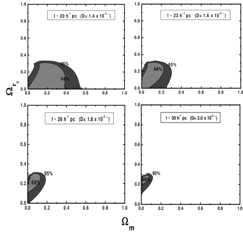
We structured this paper as follows. In Section II the basic field equations and distance formulas are presented. We also briefly discuss the predicted age of the Universe. In Section III we use measurements of the angular size of high-$z$ milliarcsecond radio sources gurv1 to constrain the free parameters of the model. We show that a good agreement between theory and observation is possible if $\Omega_{\rm{m}}\leq 0.38$, $\Omega_{\rm{r}_{c}}\leq 0.29$ and $\Omega_{\rm{m}}\leq 0.09$, $\Omega_{\rm{r}_{c}}\leq 0.29$ ($68\%$ c.l.) for values of the characteristic length of the sources between $l\simeq 20h^{-1}-30h^{-1}$ pc, respectively. In particular we find that a slightly closed, accelerated model with $\Omega_{\rm{m}}=0.06$, $\Omega_{\rm{r}_{c}}=0.28$, and $l=27.06h^{-1}$ pc is the best fit for these data.

II Field equations, distance formulas and the age of the universe

The geometry of our 4-dimensional Universe is described by the Friedmann-Robertson-Walker (FRW) line element ($c=1$)

$$ds^{2}=dt^{2}-R^{2}(t)\left[{dr^{2}\over 1-kr^{2}}+r^{2}(d\theta^{2}+\rm{sin}^{2}\theta d\phi^{2})\right],$$ (1)

where $k=0$, $\pm 1$ is the curvature parameter of the spatial section, $r$, $\theta$, and $\phi$ are dimensionless comoving coordinates, and $R(t)$ is the scale factor. The Friedmann’s equation for the kind of models we are considering is deff1 ; deffZ

$$\left[\sqrt{\frac{\rho}{3M_{pl}^{2}}+\frac{1}{4r_{c}^{2}}}+\frac{1}{2r_{c}}\right]^{2}=H^{2}+\frac{k}{R(t)^{2}},$$ (2)

where $\rho$ is the energy density of the cosmic fluid, $H$ is the Hubble parameter, $M_{pl}$ is the Planck mass, and $r_{c}=M_{pl}^{2}/2M_{5}^{3}$ is the crossover scale defining the gravitational interaction among particles located on the brane ($M_{5}$ is the 5-dimensional reduced Planck mass). For distances smaller than $r_{c}$ the force experienced by two punctual sources is the usual 4-dimensional gravitational $1/r^{2}$ force whereas for distances larger than $r_{c}$ the gravitational force follows the 5-dimensional $1/r^{3}$ behavior comm .

Equation (2) implies that the normalization condition is given by

$$\Omega_{k}+\left[\sqrt{\Omega_{\rm{r_{c}}}}+\sqrt{\Omega_{\rm{r_{c}}}+\Omega_{\rm{m}}}\right]^{2}=1$$ (3)

where $\Omega_{\rm{m}}$ and $\Omega_{k}$ are the matter and curvature density parameters, respectively and

$$\Omega_{\rm{r_{c}}}=1/4r_{c}^{2}H^{2},$$ (4)

is the density parameter associated to the crossover radius $r_{c}$.

The deceleration parameter, usually defined as $q_{o}=-R\ddot{R}/\dot{R}^{2}|_{t_{o}}$, now takes the following form

$$q_{o} = \frac{3}{2}\Omega_{\rm{m}}\left[1+\sqrt{\frac{\Omega_{\rm{r_{c}}}}{\Omega_{\rm{r_{c}}}+\Omega_{\rm{m}}}}\right]$$

$$\quad\quad\quad\quad\quad\quad-\left[\sqrt{\Omega_{\rm{r_{c}}}}+\sqrt{\Omega_{\rm{r_{c}}}+\Omega_{\rm{m}}}\right]^{2}.$$

For $\Omega_{k}=0$ (flat case), the above expression reduces to

$$q_{o}=\frac{3}{2}\Omega_{\rm{m}}\left[1+\sqrt{\frac{\Omega_{\rm{r_{c}}}}{\Omega_{\rm{r_{c}}}+\Omega_{\rm{m}}}}\right]-1.$$ (6)

Figure 1: Deceleration parameter as a function of redshift for some selected values of $\Omega_{\rm{m}}$ and $\Omega_{\rm{r_{c}}}$. The current best fit $\Lambda$CDM case is also shown for comparison. The horizontal line labeled decelerating/accelerating ($q_{o}=0$) divides models with a decelerating or accelerating expansion at a given redshift.

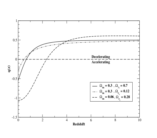
Figure 1 shows the behavior of the deceleration parameter as a function of redshift for selected values of $\Omega_{\rm{m}}$ and $\Omega_{\rm{r_{c}}}$. As explained above, although there is no cosmological constant on the brane, brane-world models allows periods of accelerated expansion because the bulk gravity sees its own curvature term on the brane as a negative-pressure dark component deff1 . The best fit $\Lambda$CDM case is also showed for the sake of comparison. Note that at late times brane-cosmologies with $\Omega_{\rm{r_{c}}}=0.3$ accelerates slower than $\Lambda$CDM models with $\Omega_{\Lambda}=0.7$ and the same value of $\Omega_{\rm{m}}$. For the best fit model found in Ref. deffZ , i.e., $\Omega_{\rm{m}}=0.3$ and $\Omega_{\rm{r_{c}}}=0.12$, the accelerated expansion begins at $z\simeq 0.5$ whereas for $\Lambda$CDM we find $z\simeq 0.7$. For our best fit, found in Section 3, we see that the Universe always accelerates at a faster rate than the best fit $\Lambda$CDM model. In this case, the Universe begins to accelerate at $z\simeq 2.3$ (see also sahini for a more detailed discussion on this topic).

From Eqs. (1) and (2), it is straightforward to show that the comoving distance $r(z)$ is given by

$$r(z)=\frac{1}{R_{o}H_{o}|\Omega_{k}|^{1/2}}\sum\left[|\Omega_{k}|^{1/2}\int_{x^{\prime}}^{1}{dx\over x^{2}f(\Omega_{j},x)}\right],$$ (7)

where the subscript $o$ denotes present day quantities, $x^{\prime}={R(t)\over R_{o}}=(1+z)^{-1}$ is a convenient integration variable and the function $\sum(r)$ is defined by one of the following forms: $\sum(r)=\mbox{sinh}(r)$, $r$, and $\mbox{sin}(r)$, respectively, for open, flat and closed geometries. The dimensionless function $f(\Omega_{j},x)$ takes the following form:

$$f(\Omega_{j},x)=\left[\Omega_{k}x^{-2}+\left(\sqrt{\Omega_{\rm{r_{c}}}}+\sqrt{\Omega_{\rm{r_{c}}}+\Omega_{\rm{m}}x^{-3}}\right)^{2}\right]^{1/2},$$ (8)

where $j$ stands for $m$, $r_{c}$ and $k$.

Figure 2: Dimensionless age parameter as a function of $\Omega_{\rm{m}}$ for some selected values of $\Omega_{\rm{r_{c}}}$. As explained in the text, for a fixed value of $\Omega_{\rm{m}}$ the larger the contribution of $\Omega_{\rm{r_{c}}}$ the larger the age predicted by the model.

Similarly, the predicted age of the Universe as a function of the redshift can be written as

$$t_{z}=H_{o}^{-1}\int_{0}^{x^{\prime}}{dx\over xf(\Omega_{j},x)}.$$ (9)

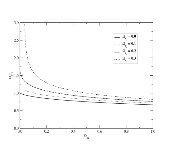
As one may check from Eqs. (2), (5), (7) and (9), for $\Omega_{\rm{r_{c}}}=0$, the standard relations are recovered. In Fig. 2 we show the dimensionless age parameter $H_{o}t_{o}$ as a function of $\Omega_{\rm{m}}$ for several values of $\Omega_{\rm{r_{c}}}$. Note that for a fixed value of $\Omega_{\rm{m}}$ the predicted age of the Universe is larger for larger values of $\Omega_{\rm{r_{c}}}$, thereby showing, similarly to what happens in the $\Lambda$CDM context, that the class of models studied here is efficient to solve the “already” classical age of the Universe problem. For example, if $\Omega_{\rm{m}}=0.3$, as sugested by dynamical estimates on scales up to about $2h^{-1}$ Mpc calb , and $\Omega_{\rm{r_{c}}}=0.15$ we find $t_{o}\simeq 13$ Gyr ($H_{o}=70{\rm{Km.s^{-1}.Mpc^{-1}}}$) or, in terms of the age parameter, $H_{o}t_{o}\simeq 0.93$, a value that is compatible with the most recent age estimates of globular clusters carreta ; chab as well as very close to some determinations based on SNe Ia data riess ; tonry .

Figure 3: Angular size vs redshift diagram for milliarcsecond radio sources data of Gurvits et al. [24]. The curves correspond to characteristic linear size $l=27.06h^{-1}$ pc (D = 1.84 mas). Thick solid curve is the prediction of the standard open model $\Omega_{\rm{r_{c}}}=0$.

III Constraints from high-$z$ angular size measurements

In this section we study the constraints from angular size measurements of high-$z$ radio sources on the free parameters of the model. In the following we briefly outline our main assumptions for this analysis. Our approach is based on Ref. alcaniz .

The angular size-redshift relation for a rod of characteristic length $l$ can be written as sand

$$\theta(z)=\frac{D(1+z)}{r(z)}.$$ (10)

In the above expression $D=100lh$ is the angular size scale expressed in milliarcsecond (mas) for $l$ measured in parsecs (compact sources).

In order to constrain the parameters $\Omega_{\rm{m}}$ and $\Omega_{\rm{r_{c}}}$ we use the angular size data for milliarcsecond radio sources recently compiled by Gurvits et al. gurv1 . This data set, originally composed by 330 sources distributed over a wide range of redshifts ($0.011\leq z\leq 4.72$), was reduced to 145 sources with spectral index $-0.38\leq\alpha\leq 0.18$ and total luminosity $Lh^{2}\geq 10^{26}$ W/Hz in order to minimize any possible dependence of angular size on spectral index and/or linear size on luminosity. This new subsample was distributed into 12 bins with 12-13 sources per bin. Two points, however, should be stressed before discussing the resulting diagrams. First of all, the determination of cosmological parameters is strongly dependent on the characteristic length $l$ (see, e.g., alcaniz ). In the absence of a statistical study describing the intrinsic length distribution of the sources, we follow alcaniz and, instead of assuming a specific value for the mean projected linear size, we have worked on the interval $l\simeq 20h^{-1}-30h^{-1}$ pc, i.e., $l\sim O(40)$ pc for $h=0.65$, or equivalently, $D=1.4-2.0$ mas (see also gurv for a detailed discussion on this topic). Second, following Kellermann kelle , we assume that compact radio sources are free of the evolutionary and selection effects that have bedevilled attempts to use extended double radio source in this context (see, for exemple, buc ), as they are deeply embedded in active galact nuclei, and, therefore, their morphology and kinematics do not depend considerably on the changes of the intergalactic medium. Moreover, these sources have typical ages of some tens of years, i.e., it is reasonable to suppose that a stable population is estabilished, characterized by parameters that do not change with the cosmic epoch jack .

Following a procedure similar to that described in alcaniz , we determine the cosmological parameters $\Omega_{\rm{m}}$ and $\Omega_{\rm{r_{c}}}$ through a $\chi^{2}$ minimization for a range of $\Omega_{\rm{m}}$ and $\Omega_{\rm{r_{c}}}$ spanning the interval [0, 1] in steps of 0.02,

$$\chi^{2}(l,\Omega_{\rm{m}},\Omega_{\rm{r_{c}}})=\sum_{i=1}^{12}{\frac{\left[\theta(z_{i},l,\Omega_{\rm{m}},\Omega_{\rm{r_{c}}})-\theta_{oi}\right]^{2}}{\sigma_{i}^{2}}},$$ (11)

where $\theta(z_{i},l,\Omega_{\rm{m}},\Omega_{\rm{r_{c}}})$ is given by Eqs. (7) and (10) and $\theta_{oi}$ is the observed values of the angular size with errors $\sigma_{i}$ of the $i$th bin in the sample.

Figure 4: Confidence regions in the $\Omega_{\rm{m}}-\Omega_{\rm{r_{c}}}$ plane according to the updated sample of angular size data of Gurvits et al. [24]. Solid lines in each panel show contours of constant likelihood (95$\%$ and 68$\%$).

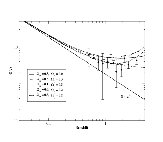
In Fig. 3 we show the binned data of the median angular size plotted as a function of redshift for several values of $\Omega_{\rm{m}}$ and $\Omega_{\rm{r_{c}}}$. For comparison we also show the standard prediction (thick line). Fig. 4 displays the $95\%$ and $68\%$ c.l. limits from angular size data on the $\Omega_{\rm{m}}-\Omega_{\rm{r_{c}}}$ plane for the interval $l\simeq 20h^{-1}-30h^{-1}$ pc. Note that the limits on the plane are more restrictive for increasing values of the characteristic length $l$. It happens because for $z\sim 2$ (where most of our data points are concentrated) the parameter $\Omega_{\rm{r_{c}}}$ has a behavior similar to a cosmological constant or quintessence, i.e., it increases the distance between two different redshifts. In this way, according to Eq. (10), for the same $\theta_{oi}$’s the larger the value of $l$ the larger the value of $r(z)$ that is required or, equivalently, the smaller the value of $\Omega_{\rm{m}}$. For $l=20.58h^{-1}$ pc (D = 1.4 mas) the peak of likelihood is located at $\Omega_{\rm{m}}=0.22$ and $\Omega_{\rm{r_{c}}}=0.18$. This assumption provides $\Omega_{\rm{m}}\leq 0.38$ and $\Omega_{\rm{r_{c}}}\leq 0.29$ at 1$\sigma$. In the subsequent panels of the same figure similar analyses are displayed for $l=23.53h^{-1}$ pc (D = 1.6 mas), $l=26.47h^{-1}$ pc (D = 1.8 mas) and $l=29.41h^{-1}$ pc (D = 2.0 mas). For an analysis independent of the choice of the characteristic length $l$, i.e., minimizing Eq. (11) for $\Omega_{\rm{m}}$, $\Omega_{\rm{r_{c}}}$ and $l$, we obtain $\Omega_{\rm{m}}=0.06$, $\Omega_{\rm{r_{c}}}=0.28$ and $l=27.06h^{-1}$ pc (D = 1.84 mas) as the best fit for these data with $\chi^{2}=4.25$ and 9 degrees of freedom. We also remark that although not discussed here it is possible to determine the influence of $\Omega_{\rm{r_{c}}}$ on the critical redshift $z_{m}$ at which the angular size takes its minimal value. However as shown elsewhere jailS , this test cannot discriminate among world models since different scenarios provide similar values of $z_{m}$.

An elementary combination of our best fit with Eq. (4) enables us to estimate $r_{c}$ (the crossover distance between 4-dimensional and 5-dimensional gravity) in terms of the Hubble radius $H_{o}^{-1}$. One obtains,

$$r_{c}\simeq 0.94H_{o}^{-1}.$$ (12)

Such a value is slightly different from that one found by Deffayett et al. deff using SNe Ia and CMB data. In their analysis it was found as a concordance model for these two tests a flat model with $\Omega_{\rm{m}}=0.3$ and $\Omega_{\rm{r_{c}}}=0.122$, leading to an estimate of the crossover radius of $r_{c}\simeq 1.4H_{o}^{-1}$. Naturally, with new results from different cosmological tests it will be possible to delimit the $\Omega_{\rm{m}}-\Omega_{\rm{r_{c}}}$ plane more precisely. An analysis on the observational constraints from statistics of gravitational lenses will appear in a forthcoming communication alc .

IV conclusion

Based on a large body of observational evidence, a consensus is beginning to emerge that we live in a flat, accelerated universe composed of $\sim$ 1/3 of matter (barionic + dark) and $\sim$ 2/3 of a negative-pressure dark component. However, since the nature of this dark energy is still not well understood, an important task nowadays in cosmology is to investigate the existing possibilities in the light of the current observational data. In this paper we have focused our attention on some observational aspects of brane world cosmologies. These models, inspired on superstring-M theory, explain the observed acceleration of the Universe through a large scale modification of gravity arising from a gravitational leakage into an extra dimension deffZ . We showed that their predicted age of the Universe is compatible with the most recent age estimates of globular clusters and, therefore, that there is no age crisis in the context of these models. By using a large sample of milliarcsecond radio sources recently updated and extended by Gurvits et al. gurv1 we obtained, as the best fit for these data, a slightly closed, accelerated universe with $\Omega_{\rm{m}}=0.06$ and $\Omega_{\rm{r_{c}}}=0.28$. Such values lead to an estimate of the crossover radius of $r_{c}\simeq 0.94H_{o}^{-1}$.