Cosmological Magnetic Fields from Primordial Helical Seeds

Abstract

Most early Universe scenarios predict negligible magnetic fields on cosmological scales if they are unprocessed during subsequent expansion of the Universe. We present a new numerical treatment of the evolution of primordial fields and apply it to weakly helical seeds as they occur in certain early Universe scenarios. We find that initial helicities not much larger than the baryon to photon number can lead to fields of $\sim 10^{-13}\,$G with coherence scales slightly below a kiloparsec today.

I Introduction

The origin of galactic and large scale extragalactic magnetic fields (for which there is no detection yet on scales larger than mega-parsecs) is one of the main unresolved problems of astrophysics and cosmology review . In most scenarios where magnetic fields are produced in the early Universe, these seed fields are concentrated on scales below the horizon scale where they dissipate quickly, and are too small on cosmological scales to have any observable effects. However, if pseudoscalar interactions induce a non-vanishing helicity of these seeds, such as in string cosmology string or during the electroweak phase transition by projection of non-abelian Chern-Simons number onto the electromagnetic gauge group ew ; cornwall ; vachaspati , then part of the small scale power can cascade to large scales and produce observable effects cascade ; cornwall ; son ; fc . In this paper we develop a new numerical approach to treat such non-linear cascades up to zero redshift and apply it to helical seed fields produced in the early Universe.

II MHD in the Early Universe

The principal equations for magnetic field ${\bf B}$ and velocity field ${\bf v}$ in the one-fluid approximation of magnetohydrodynamics (MHD) are choudhuri

$$\partial_{t}{\bf B} = {\bf\nabla}\times({\bf v}\times{\bf B}-\eta\,{\bf\nabla}\times{\bf B})\,$$

$$\partial_{t}{\bf v}+({\bf v}\cdot{\bf\nabla}){\bf v} = \frac{({\bf\nabla}\times{\bf B})\times{\bf B}}{4\pi\rho}\,,$$ (1)

where $\eta$ is the resistivity and $\rho$ is the fluid density. The second equation describes backreaction of the magnetic field on the flow. To eliminate it, following Ref. subra ; cornwall , we write

$${\bf v}\sim\frac{{\bf f}}{\beta\rho}=\frac{\tau}{4\pi\rho}({\bf\nabla}\times{\bf B})\times{\bf B}\,,$$ (2)

where $\beta$ is the drag coefficient and $\tau\equiv 1/\beta$ is the fluid response time to the Lorentz force ${\bf f}=\left[({\bf\nabla}\times{\bf B})\times{\bf B}\right]/(4\pi)$. The latter can be viewed as the time the charged fluid can be accelerated until it interacts (scatters) with other particles in the background and therefore describes damping of the magnetic field modes.

Again following Ref. subra , we express the magnetic field in terms of correlation functions $M_{ij}(r,t)=\left\langle B_{i}({\bf x},t)B_{j}({\bf y},t)\right\rangle$, where $r=|{\bf x}-{\bf y}|$, assuming isotropy and homogeneity,

$$M_{ij}=M_{N}\left(\delta_{ij}-\frac{r_{i}r_{j}}{r^{2}}\right)+M_{L}\frac{r_{i}r_{j}}{r^{2}}+H\epsilon_{ijk}r_{k}\,$$ (3)

where $M_{L}$, $M_{N}$, and $H$ are longitudinal, transverse, and helical magnetic correlation functions, respectively. $M_{N}=\partial_{r}(r^{2}M_{L})/(2r)$ is not independent because of ${\bf\nabla}\cdot{\bf B}=0$. We define the magnetic field and gauge invariant helicity power spectra per logarithmic wavenumber interval $b^{2}(k)$ and $h(k)$ by $E_{M}\equiv\left\langle{\bf B}^{2}({\bf r})\right\rangle/(8\pi)=\int_{0}^{+\infty}dkb^{2}(k)/(8\pi k)$ and $H_{M}\equiv\left\langle{\bf B}({\bf r})\cdot{\bf A}({\bf r})\right\rangle=\int_{0}^{+\infty}dkh(k)/k$, with ${\bf A}$ the vector potential, ${\bf B}={\bf\nabla}\times{\bf A}$. One can show that $M_{L}$ and $H$ are related to these power spectra via

$$M_{L}(r) = \int_{0}^{+\infty}\frac{dk}{k}\frac{j_{1}(kr)}{kr}b^{2}(k)$$

$$H(r) = -\frac{1}{3r}\int_{0}^{+\infty}dk\,j_{1}(kr)h(k)\,,$$ (4)

where $j_{1}(x)=\sin(x)/x^{2}-\cos(x)/x$ is the first order spherical Bessel function. In terms of the usual Fourier transforms ${\bf B}({\bf k})=\int d^{3}{\bf r}/(2\pi)^{3/2}\exp(i{\bf k}\cdot{\bf r}){\bf B}({\bf r})$ etc., $b^{2}(k)=4\pi k^{3}{\bf B}^{2}(k)$ and $h(k)=k^{3}\int d\Omega_{\bf k}{\bf B}({\bf k})\cdot{\bf A}({\bf k})$. Eq. (4) also shows that $M_{L}(0)=8\pi E_{M}/3$, and $H_{M}=-3\int_{0}^{+\infty}drrH(r)$, and $|h(k)|\leq b^{2}(k)/k$ implies for all $r$

$$|H(r)|\lesssim|M_{L}(r)|/r\equiv H_{\rm max}(r)\,.$$ (5)

Cosmological expansion can be taken into account by redefining $M_{L}\to M_{L}/T^{4}$ and $H\to H/T^{5}$ from now on, where $T$ is the cosmological temperature. Assuming for now the absence of any external source terms such as fluid motions except the one induced by the magnetic field, i.e. using Eq. (2), the MHD equations (1) reduce to

$$\partial_{t}M_{L} = \frac{2}{r^{4}}\partial_{r}\left(r^{4}\kappa\partial_{r}M_{L}\right)-4\alpha TH$$

$$\partial_{t}H = \frac{1}{r^{4}}\partial_{r}\left[r^{4}\partial_{r}\left(2\kappa H+\alpha M_{L}/T\right)\right]$$ (6)

where

$$\kappa = \eta+\frac{\tau T^{4}}{2\pi\rho}M_{L}(0,t)$$

$$\alpha = -\frac{\tau T^{5}}{\pi\rho}H(0,t)\,,$$ (7)

and all quantities appearing here are in physical (not co-moving) coordinates. The diffusion term $\kappa$ consists of a microscopic ($\eta$) and a non-linear drift contribution, whereas the $\alpha$ effect is only due to non-linear drift here. The source terms will be discussed in the next section. If the spatial derivatives of $M_{L}$ and $H$ fall off faster than $1/r$ for $r\to\infty$, Eq. (6) implies $\partial_{t}H_{M}=9\left[2\kappa H(0)+\alpha M_{L}(0)\right]$ which, together with Eq. (7), shows that helicity is conserved in the absence of resistivity.

Eqs. (6) describe small and large scale dynamos of helical magnetic fields including damping by Ohmic dissipation and ”Silk” damping (which is expressed by the redshift dependent relaxation time $\tau$) on a unified basis. In the early Universe the resistivity can be estimated by $\eta\simeq 1/(40\pi T)$ before photon decoupling, $T\gtrsim 0.25\,$eV ae , and by the Spitzer resistivity $\eta\simeq\pi m_{e}^{1/2}e^{2}/T_{e}^{3/2}$ (where $m_{e}$, $e$, and $T_{e}\sim 10^{6}\,$K are electron mass, charge, and temperature, assuming full ionization) after recombination choudhuri (the results are insensitive to the latter). Below $e^{+}e^{-}$ annihilation at $T\simeq 20\,$keV, within the MHD one fluid approximation the fluid coupled to the magnetic field is well represented by the tightly coupled remaining free electrons and protons and $\tau$ is governed by Thomson scattering of photons off electrons. In this regime we use jko1

$$\tau = \tau_{\gamma}\simeq 4\times 10^{21}\left(\frac{0.25{\rm eV}}{T}\right)^{4}\,X_{e}^{-1}\,{\rm cm}$$

$$\frac{\rho}{T^{4}} \simeq 0.4\frac{4\pi^{2}}{45}\left(\frac{0.25{\rm eV}}{T}\right)\left(\frac{\Omega_{b}h^{2}}{0.0125}\right)\,,$$ (8)

where the number of free electrons per nucleon $X_{e}$ is $\simeq 1$ for $T\gtrsim 0.25\,$eV and $\simeq 10^{-5}$ for $T\lesssim 0.25\,$eV, and $\Omega_{b}h^{2}$ is the baryon density in terms of the critical density times the Hubble constant in units of $100\,{\rm km}/{\rm s}/{\rm Mpc}$ today. For $T\gtrsim 20\,$keV we can approximate the fluid to consist of the electromagnetically interacting particles and $\tau$ is governed by neutrino scattering with jko1

$$\tau=\tau_{\nu}\simeq 10^{11}\left(\frac{{\rm MeV}}{T}\right)^{5}\frac{8.75}{g_{r}-2}\frac{g_{r}}{g_{\nu}}\,{\rm cm}\,,$$ (9)

and $\rho/T^{4}\simeq g_{f}\pi^{2}/30$, where $g_{r}$, $g_{f}$, and $g_{\nu}=5.25$ are the statistical weights of all relativistic particles, the particles in the fluid and of the neutrinos, respectively.

III Helical Seeds

Here we consider helical fluid motion, as it can arise during cosmological phase transitions (see, for example, Ref. ew ; cornwall for the electroweak phase transition). This case has already been treated in Ref. subra which we adapt here to our situation. Since the backreaction of the magnetic field onto the fluid motion has already been taken into account by the approximation Eq. (2), the external fluid flow ${\bf v}_{e}$ is assumed to be uncorrelated with the field. It is furthermore assumed that the correlation time of the external velocity field is much smaller than the time scale of change of the magnetic correlation function, $\left\langle{\bf v}_{ei}({\bf x},t){\bf v}_{ej}({\bf y},s)\right\rangle=T_{ij}(r)\delta(t-s)$, where, in analogy to Eq. (3), $r=|{\bf x}-{\bf y}|$, and

$$T_{ij}=T_{N}\left(\delta_{ij}-\frac{r_{i}r_{j}}{r^{2}}\right)+T_{L}\frac{r_{i}r_{j}}{r^{2}}+C\epsilon_{ijk}r_{k}\,.$$ (10)

Assuming for simplicity an incompressible fluid, ${\bf\nabla}\cdot{\bf v}_{e}=0$, the additional terms in Eqs. (6) and (7) are given by

$$\partial_{t}M_{L} = \cdots-\left(2\partial_{r}^{2}T_{L}+\frac{8}{r}\partial_{r}T_{L}\right)M_{L}$$

$$\kappa = \cdots+T_{L}(0)-T_{L}(r)$$ (11)

$$\alpha = \cdots+2C(0)-2C(r)\,,$$

such that $\kappa$ and $\alpha$ obtain a scale dependent turbulent diffusion and $\alpha$ effect contributions, respectively, from the fluid. Here $T_{L}$ and $C$ are given by $T_{L}(r)=\tau_{\rm corr}\left\langle{\bf r}\cdot{\bf v}_{e}(0){\bf r}\cdot{\bf v}_{e}({\bf r})\right\rangle/r^{2}$ and $C(r)=\tau_{\rm corr}\left\langle{\bf r}\cdot{\bf v}_{e}(0)\times{\bf v}_{e}({\bf r})\right\rangle/(2r^{2})$. The correlation time $\tau_{\rm corr}$ is either the damping time scale due to interactions with the background or, if all components are tightly coupled and move as a whole, the age of the Universe $t_{u}(T)$ at the relevant epochs.

The spatial velocity correlations $T_{L}$ and $C$ can be expressed in terms of their power spectra $v^{2}(k)$ and $c(k)$, respectively, in complete analogy to Eq. (4). In general they will have the form

$$T_{L}(r) = \frac{1}{3}\tau_{\rm corr}\left\langle v_{e}^{2}\right\rangle(T)f(r)$$

$$|C(r)| \lesssim |T_{L}(r)|/r\equiv C_{\rm max}(r)\,,$$ (12)

where $f(r)$ is a dimensionless function with $f(r)\to 1$ for $r\to 0$ and, typically, a power law fall-off at large distances, and the total power $\left\langle v_{e}^{2}\right\rangle(T)$ typically peaks at a certain temperature $T_{\rm ph}$, for example, at a primordial phase transition, and becomes negligible for $T\gg T_{\rm ph}$ and $T\ll T_{\rm ph}$.

IV Numerical Simulations and Results

For any early Universe scenario the initial conditions for $M_{L}$ and $H$ at the temperature where the fields are created should be calculated from the power spectra $b^{2}(k)$ and $h(k)$, using Eq. (4). The magnetic field evolution can then be obtained by numerically integrating the non-linear partial differential Eqs. (6) and their extensions with helical source terms in co-moving coordinates from this initial time up to redshift zero. This is done by employing an alternating implicit method recipes to a one-dimensional grid of typically a hundred bins roughly logarithmic in co-moving distance between the inverse of today’s cosmic microwave background (CMB) temperature $T_{0}$ and $\sim 10^{4}\,$Mpc, and using the logarithm of the temperature $\ln T$ as independent variable, adopting the standard relations between time and temperature, see e.g. Ref. kt . In order to assure that induced velocities Eq. (2) remain non-relativistic, the induced contributions to the coefficients $\kappa$ and $\alpha$, Eq. (7), are limited to the corresponding contributions, Eq. (11), of a maximally strong external fluid flow during the simulations.

At a physical length scale $r$ at cosmic time $t$ the accuracy requirement on the step-size is recipes $\Delta\ln T\lesssim r^{2}/\left[t\,{\rm Max}(\kappa,\alpha)\right]$. For about $10^{4}$ time steps per decade in $T$ and for the coefficients given by Eq. (7) this is typically fulfilled for temperatures up to close to the GUT scale and co-moving lengths down to the parsec scale which are mostly of interest here. Although this accuracy requirement is not fulfilled at the smallest length scales close to the inverse temperature used in the numerical integration, the implicit method assures at least convergence toward the equilibrium solution at such scales.

The power spectra $b^{2}(k)$ and $h(k)$ can be obtained by inverting the transformations of Eq. (4), but a rough estimate is given by $b^{2}(k)\sim M_{L}(1/k)$ and $h(k)\sim H(1/k)/k^{2}$.

In the following we parametrize the magnetic seed field by

$$M_{L}(r)=N\frac{8\pi^{3}}{90}\frac{1}{(1+r/r_{B})^{n}}\,,$$ (13)

where $N$ characterizes the strength relative to thermal density, $r_{B}$ is the scale on which it is concentrated, and $n$ is the power law index at much larger scales (causally produced fields correspond to $n\geq 5$).

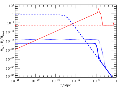
Figure 1: Results in co-moving length scale $r$ for the case without external fluid flow. Thick lines show $M_{L}(r)$ in units of $T^{4}$, for initial condition at $T=100\,$GeV (thick dashed), and at zero redshift (thick solid, i.e. $M_{L}=1$ corresponds to a field strength of $\simeq 1.4\times 10^{-6}$ Gauss today, note that $M_{L}$ is quadratic in ${\bf B}$). Thin lines show helicity relative to maximal, $h(r)\equiv H(r)/H_{\rm max}(r)$, for initial condition (thin dashed), and at zero redshift (thin solid). For comparison, the thin dotted line shows the final $M_{L}(r)$ for maximal initial helicity (not shown).

To demonstrate the general effect of helicity we start with magnetic fields of non-vanishing helicity in the absence of source terms. We start at the electroweak scale, $T=100\,$GeV, with a seed field Eq. (13) with $N=0.1$, concentrated at a scale $r_{B}=10^{-4}t_{u}(100\,{\rm GeV})$, and a power law index $n=3$, motivated by a superposition of magnetic dipoles, as may be expected for the electroweak transition soj . We assume an initial helicity $H_{M}\sim 100n_{b}$, somewhat larger than the baryon number $n_{b}$, as suggested by models cornwall ; vachaspati . Assuming the relative helicity, $h(r)\equiv H(r)/H_{\rm max}(r)$, to be roughly independent of $r$, this corresponds to $H(r)\sim 100/N(n_{b}/n_{\gamma})\,M_{L}(r)/r\simeq 5\times 10^{-7}H_{\rm max}(r)$, where the baryon to photon ratio $n_{b}/n_{\gamma}\sim 5\times 10^{-10}$. Fig. 1 shows results for $M_{L}$ and the relative helicity. The field at zero redshift is decreased by dissipation up to the $\simeq 0.1\,$parsec scale, whereas inverse cascades enhance the field on scales of a few parsecs, reaching $\sim 10^{-14}\,$G. For comparison Fig. 1 also shows the larger enhancement of $M_{L}$ for maximal initial helicity (the case discussed in Ref. fc ) which, however, we consider speculative in the absence of a specific model predicting such large helicities.

It is easy to show that the total helicity $H_{M}$ which is dominated by the peak of $h(r)$ in Fig. 1 is roughly conserved, and thus evolution is dominated by magnetic back-reaction onto the fluid. Indeed, conservation of $H_{M}$ is usually employed to estimate the field strength via $B^{2}\sim H_{M}/l_{c}$ which requires an analytical estimate of the coherence scale $l_{c}$ vachaspati . In our numerical approach $l_{c}$ comes out without further assumptions as the scale where the correlation function cuts off.

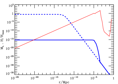
Figure 2: Results in the presence of a fully helical external fluid flow of small amplitude, $\left\langle v_{e}^{2}\right\rangle=10^{-12}$, at the electroweak transition. See Fig. 1 for line key and text for details.

Another interesting situation could be the production of baryon and lepton number comparable to unity, $n_{b}/n_{\gamma}\sim 1$ at $T=T_{n}\gg 100\,$GeV, for instance during a phase transition related to new physics, which could give rise to maximally helical flows as well. These flows would consist of the tightly coupled electroweak plasma and could survive as a small perturbation at least down to the neutrino decoupling temperature, i.e. $t_{\rm corr}\simeq t_{u}(T)$ for $T\gtrsim\,$MeV. Their amplitude can be estimated by the dilution factor $\left\langle v_{e}^{2}\right\rangle\sim(n_{b}/n_{\gamma})_{\rm today}^{4/3}\sim 10^{-12}$ due to the necessary entropy production above the electroweak scale. Assuming a causal flow with power on scales not too far below the horizon scale, we use $f(r)=[1+rT/t_{u}(T_{n})/T_{n}]^{-5}$ with $T_{n}=10^{13}\,$GeV for the other parameters in Eq. (12). We start with the same magnetic field produced at the electroweak transition as above, but this time with vanishing initial helicity, $H(r)\equiv 0$. Fig. 2 shows that in this case the magnetic field develops helicity and reaches values close to $10^{-13}\,$G up to about 100 parsecs. The coherence scales are also consistent with analytical estimates son ; fc , but are considerably larger than in Ref. vachaspati .

Our results also demonstrate that the presence of helicity prevents complete dissipation of the fields at small scales, resulting in a flat correlation function up to the coherence scale. Furthermore, the relative magnetic helicity rises linearly with $r$ and is close to maximal at the coherence scale. This could have ramifications for the actual detection of helicity, for example, via its effects on the CMB pvw and could be an important signature of physics at or above the electroweak scale.

V Conclusions

We used the evolution equations for the two-point correlation function of helical magnetic fields in MHD approximation including magnetic diffusion, fluid viscosity, and back-reaction onto the external fluid to evolve weakly helical fields produced in the early Universe up to today. We find that magnetic fields and/or fluid flows with a helicity relative to maximal not much larger than the baryon to photon number $\sim 10^{-9}$, as expected during the electroweak period, can lead to significant inverse cascades. This results in magnetic fields that can be enhanced by several orders of magnitude compared to the merely red-shifted and frozen-in initial fields at scales in the parsec and kilo-parsec range today. If the seeds are roughly thermal in strength and if their power is concentrated on scales not much smaller than the horizon scale around the electroweak transition, the coherence length is close to a kilo-parsec with field strengths up to $\,10^{-13}\,$G. While this is smaller than the analytical estimates in Refs. fc , it is based on the more realistic assumptions of small helicities of order the baryon to photon number where fluid viscosity can not be neglected. The fields we obtain are certainly larger than from “astrophysical” seed field mechanisms such as the Biermann battery, but are also well within the limits from big bang nucleosynthesis and the CMB (the best of which are $\sim 10^{-9}\,$Gauss on kpc–Mpc scales, see, e.g., lk ; sb ; jko ), and from gravity wave production ($B(r)\lesssim 10^{-11}(r/100\,{\rm pc})^{-3}$ for $n=3$ cd ). Such fields may also be testable by ultra-high energy cosmic ray deflection bs . The approach presented here can also be applied to other magneto-genesis scenarios with pseudo-scalar seeds such as in string cosmology ss where coupling to axions may lead to larger helicities.

Acknowledgments I would like to thank A. Buonanno, K. Jedamzik, and M. Sakellariadou for helpful discussions.

References

- (1) for a review see, e.g., D. Grasso and H. Rubinstein, Phys. Rept. 348 (2001) 163.
- (2) see, e.g., D. Lemoine and M. Lemoine, Phys. Rev. D 52 (1995) 1955; R. Durrer and M. Sakellariadou, Phys. Rev. D 62 (2000) 123504.
- (3) R. Jackiw and So-Young Pi, Phys. Rev. D 61 (2000) 105015.
- (4) J. M. Cornwall, Phys. Rev. D 56 (1997) 6146
- (5) T. Vachaspati, Phys. Rev. Lett. 87 (2001) 251302.
- (6) see, e.g., K. Enqvist, Int. J. Mod. Phys. D7 (1998) 331.
- (7) D. T. Son, Phys.Rev. D 59 (1999) 063008;
- (8) G. B. Field and S. M. Carroll, Phys. Rev. D 62 (2000) 103008.
- (9) see, e.g., R. Choudhuri, The Physics of Fluids and Plasmas: An Introduction for Astrophysicists (Cambridge University Press, 1999).
- (10) K. Subramanian, Phys. Rev. Lett. 83 (1999) 2957; Phys. Rev. Lett. 83 (1999) 2957.
- (11) J. Ahonen and K. Enqvist, Phys. Lett. B 382 (1996) 40.
- (12) K. Jedamzik, V. Katalinic, and A. Olinto, Phys. Rev. D 57 (1998) 3264.
- (13) W. H. Press, S. A. Teukolsky, W. T. Vetterling, and B. P. Flannery, Numerical Recipes in Fortran (Cambridge University Press, 1992).
- (14) E. W. Kolb and M. S. Turner, The Early Universe (Addison-Wesley, Redwood City, California, 1990).
- (15) G. Sigl, A. Olinto, and K. Jedamzik, Phys. Rev. D 55 (1997) 4582.
- (16) L. Pogosian, T. Vachaspati, and S. Vinitzki, e-print astro-ph/0112536.
- (17) A. Loeb and A. Kosowsky, Astrophys. J. 469 (1996) 1.
- (18) K. Subramanian and J. D. Barrow, Phys. Rev. Lett. 81 (1998) 3575.
- (19) K. Jedamzik, V. Katalinic, and A. Olinto, Phys. Rev. Lett. 85 (2000) 700.
- (20) C. Caprini and R. Durrer, Phys. Rev. D 65 (2002) 023517.
- (21) for a review see, e.g., P. Bhattacharjee and G. Sigl, Phys. Rept. 327 (2000) 109.
- (22) M. Sakellariadou and G. Sigl, in preparation.