The Galactic Distribution of Asymptotic Giant Branch Stars
Abstract
We study the Galactic distribution of 10,000 Asymptotic Giant Branch (AGB) stars selected by IRAS colors and variability index. The distance to each star is estimated by assuming a narrow luminosity function and a model-derived bolometric correction. The characteristic AGB star luminosity, , is determined from the condition that the highest number density must coincide with the Galactic bulge. Assuming a bulge distance of 8 kpc, we determine 3,500 L⊙, in close agreement with values obtained for nearby AGB stars using the HIPPARCOS data.
We find that there are no statistically significant differences in the Galactic distribution of AGB stars with different IRAS colors, implying a universal density distribution. The direct determination of this distribution shows that it is separable in the radial, , and vertical, , directions. Perpendicular to the Galactic plane, the number density of AGB stars is well described by an exponential function with a vertical scale height of 300 pc. In the radial direction the number density of AGB stars is constant up to 5 kpc, and then it decreases exponentially with a scale length of 1.6 kpc. This fall-off extends to at least 12 kpc, where the sample becomes too small. The overall normalization implies that there are about 200,000 AGB stars in the Galaxy.
We estimate the [25]-[12] color distribution of AGB stars for an unbiased volume-limited sample. By using a model-dependent transformation between the color and mass-loss rate, , we constrain the time dependence of . The results suggest that for 10-6 M⊙yr M⊙yr-1 the mass-loss rate increases exponentially with time. We find only marginal evidence that the mass-loss rate increases with stellar mass.
keywords:
stars: asymptotic giant branch — stars: mass-loss — stars: evolution — Milky Way galaxy — Infrared Astronomical Satellite1 Introduction
Studies of the stellar distribution within the Galaxy can provide information on its formation mechanism(s) and subsequent evolution. While a significant amount of data about the Galaxy has been collected over the years, the knowledge about the stellar distribution in the Galactic plane is still limited to a few kpc from the Sun (Mihalas & Binney 1981, Binney & Tremaine 1987) by interstellar dust extinction because the visual extinction is already 1 mag at a distance of only about 0.6 kpc (Spitzer, 1978).
The interstellar dust extinction decreases with wavelength and is all but negligible beyond about 10 m, even for stars at the Galactic center. For this reason, the analysis of the data obtained by the Infrared Astronomical Satellite (IRAS, Beichman et al. 1985) has significantly enhanced our knowledge of the stellar distribution in the Galactic disk and bulge. IRAS surveyed 96% of the sky at 12, 25, 60 and 100 m, with the resulting point source catalog (IRAS PSC) containing over 250,000 sources. The colors based on IRAS fluxes111Except when discussing bolometric flux, the implied meaning of “flux” is the flux density. can efficiently be used to distinguish pre-main sequence from post-main sequence stars, and to study characteristics of their dust emission (e.g. van der Veen & Habing 1987, Ivezić & Elitzur 2000, hereafter IE00).
Soon after the IRAS data became available it was realized that properly color-selected point sources clearly outline the disk and the bulge (Habing et al. 1985). The color selection corresponds to OH/IR stars, asymptotic giant branch (AGB) stars with very thick dust shells due to intensive mass loss (for a detailed review see Habing 1996). Because these stars have large luminosity ( L⊙), and because a large fraction of that luminosity is radiated in the mid-IR due to reprocessing by surrounding dust, they are brighter than the IRAS faint cutoff ( 1 Jy at 12 m) even at the distance of the Galactic center. The availability of IRAS data soon prompted several detailed studies of the Galactic distribution of AGB stars. Common features in all these studies are the sample selection based on the IRAS vs. [25]-[12] color-magnitude diagram, and the determination of the bolometric flux by utilizing a model based bolometric correction.
Habing et al. (1985) discuss 7,000 bulge stars selected by 0.5 / 1.5 and 1 Jy 5 Jy, in two areas defined by , and . Assuming that for all stars = 2.3 Jy, and a bolometric correction calculated for a T=350 K black body, they derive = 2600 L⊙(for the Galactic center distance of 8 kpc, Reid 1989). They also find that 25% of the selected sources have IRAS variability index (the probability that a source is variable, expressed in percent, for definition see Section 2.2) larger than 99, as compared to 13% for all stars from the IRAS PSC. This difference is in good agreement with the known long period variability of AGB stars. Habing et al. (1985) also noted that despite this agreement, their sample may still be severely contaminated by planetary nebulae. They classified 2% of stars from the sample using supplemental data and found the same fractions of variable stars and planetary nebulae.
Rowan-Robinson & Chester (1987) select bulge stars by requiring 1 Jy (interpreted as the IRAS confusion limit) and . They assumed that all these objects in the direction of the Galactic center are actually at the Galactic center. This assumption allowed them to determine the median luminosity (3,000 L⊙) and to place an upper limit on the width of the luminosity function, which was found to be very narrow (the root-mean-square scatter is about a factor of 2). They also determined the distribution of colors and transformed it into a distribution of the shell optical depth by using model-dependent transformations. Assuming that this luminosity function and optical depth distribution also apply to the Galactic disk, and that the disk volume density distribution can be parametrized as two separable exponential functions in the vertical, , and radial, , directions, they derive a scale height of 250 pc and a scale length of 6 kpc.
Habing (1988) extended the analysis to disk sources in several areas on the sky defined as thin strips parallel to the Galactic equator, with a total area of 1200 deg2, or about 3% of the sky. AGB stars are selected by requiring 1 Jy, 0.3 / 3.8 and q12 = q25 = 3, where q12 and q25 are IRAS flux qualities at 12 and 25 m (1=upper limit, 2=low quality, 3=high quality). Habing does not include the 60 m flux in the source selection because the resulting number of sources is too small, but does exclude those sources for which F is reliably measured. This sample was used to constrain the luminosity function and spatial distribution of stars by fitting number counts in the selected areas. The spatial distribution is assumed to be separable: a sech2 function for the direction with an -independent scale height (this was motivated by results obtained for other galaxies), and an exponential for the direction. Habing finds that the models are not unique, and it is hard to find a best-fitting one. He concludes that the sample contained two populations with either a similar spatial density and different luminosities, or a similar luminosity but different spatial distributions. Habing prefers the second option and argues that the results present evidence for the thick disk proposed by Gilmore and Reid (1983), and for a thin disk cutoff at 10 kpc. He also points out that the luminosity function in the disk is similar to that in the bulge, providing support for the earlier assumption by Rowan-Robinson and Chester (1987).
Blommaert, van der Veen & Habing (1993) extended the study by Habing (1988) with the aim of determining the sample contamination. They obtained near-IR photometry and OH maser measurements for 53 sources which are located outside the solar circle and have (region IIIb of the IRAS color-color diagram, as defined by van der Veen and Habing, 1988). Although this subsample is expected to have the least amount of contamination by non-AGB stars, they find that 55% of objects are not AGB stars. The contaminating sources have overestimated distances due to both underestimated bolometric corrections and overestimated luminosities, and resulted in spurious evidence for a thick disk and the thin disk cutoff.
These pioneering IRAS-based studies suggested that the luminosity function for AGB stars is rather narrow and centered around 3,000 L⊙, and appears not to vary strongly with position in the Galaxy. The IRAS number counts can be reasonably well fitted by assuming a spatial distribution of AGB stars which is separable in and , and described by exponential functions with a scale height of 250 pc and a scale length of 6 kpc, respectively.
In this work we revisit the problem of constraining the Galactic distribution of AGB stars using IRAS data. There are several factors motivating us to perform a study similar to those listed above:
-
1.
The study by Blommaert, van der Veen & Habing (1993) showed that the variability index is a reliable indicator of AGB stars, while samples selected by colors alone can be significantly contaminated. Thus, it seems prudent to complement the sample color selection by using the IRAS variability index and repeat the analysis. Further, the understanding of the IRAS color-color diagrams and the distribution of various types of dusty star has advanced since the early studies of IRAS data, and can be used to select cleaner, more reliable samples (e.g. van der Veen & Habing 1988, IE00).
-
2.
The spectral energy distribution (SED) models for AGB stars and their dependence on the various stellar parameters are also better understood. In particular, more reliable bolometric corrections are available, and the IRAS colors are recognized as an indicator of the mass-loss rate (Habing 1996, and references therein).
-
3.
The HIPPARCOS data allowed direct determination of the bolometric luminosity for AGB stars in the solar neighborhood. The luminosity distribution of nearby AGB stars is very narrow and centered around 3,000 L⊙ (Knauer, Ivezić & Knapp 2001). Since it is very similar to the luminosity function obtained for the much redder bulge stars, it appears that the luminosity function is similar throughout the Galaxy and not very dependent on stellar color. Due to this similarity, it is possible to postulate a universal narrow luminosity function and estimate the distance to each star irrespective of its color and position in the Galaxy. This allows a direct study of their galactic distribution, rather than constraining it indirectly by modeling the number counts vs. flux relation.
-
4.
All previous studies assumed that the number density distribution is separable in and . Although the available IRAS data appear sufficient to explicitly test this assumption, this has not yet been done. In addition, subsamples of AGB stars with different colors (reflecting different mass-loss rates) can be formed, allowing a study of differences in their Galactic distribution.
In Section 2 we discuss the IRAS data and the method developed for selecting AGB stars. The determination of the Galactic distribution of 10,000 selected stars is described in Section 3, and in Section 4 we analyze the time evolution of AGB mass loss. The results are summarized and discussed in 5.
2 Selection Method
2.1 The IRAS PSC Data

The IRAS color-color and color-magnitude diagrams have been extensively used to select and classify various types of dusty star (e.g. van der Veen and Habing 1988, Walker et al. 1989). Most recently, IE00 showed that all IRAS sources can be separated into 4 classes, including AGB stars. They obtain a very clean classification by using a scheme which requires at least 3 IRAS fluxes. For AGB stars the three best fluxes typically are 12 m, 25 m, and 60 m fluxes. However, as already pointed out by Habing (1988), the requirement that the IRAS flux at 60 m be of good quality significantly decreases (by more than a factor 4) the number of available sources. Further, even for stars with formally good 60 m flux, there is significant contamination by interstellar cirrus emission (Ivezić & Elitzur 1995, hereafter IE95). For this reason, we are forced to use only the IRAS fluxes at 12 m and 25 m, and the resulting color [25]-[12] = log(/).
There are 88,619 sources in the IRAS PSC with both the 12 m and 25 m flux qualities greater than 1. Their [25]-[12] color and flux distributions are shown in the top two panels in Figure 1. The right panel indicates that the sample is complete to 1 Jy. The left panel shows the color distribution for 64,329 sources with 1 Jy. There are two obvious peaks. The peak at [25]-[12] = -0.6 represents stars without dust emission, and the peak at [25]-[12] = -0.25 is dominated by AGB stars (IE00).
The color and flux distributions of the stars in the sample are very dependent on the galactic coordinates. The two panels in the second row in Figure 1 show the color and flux distributions for a subsample of 1,022 stars towards the galactic poles () compared to the color distribution of the whole sample. As evident, the sample is dominated by dust-free stars. On the contrary, the disk stars and stars towards the bulge are dominated by AGB stars, as evident in the panels in the last two rows. The strong dependence of the color and flux distributions on the galactic coordinates indicates the rich information on the Galactic structure encoded in these data.
2.2 The AGB Sample Selection Criteria

Figure 2 in IE00 shows that sources with [25]-[12] -0.2 are dominated by AGB stars, and that their fraction becomes negligible for [25]-[12] 0.2, where the sample is dominated by young stellar objects. An optimal separation line between the AGB stars and other sources (mostly young stellar objects and planetary nebulae) is [25]-[12]=0. While it is tempting to define the sample by using only this criterion, Blommaert, van der Veen & Habing (1993) showed that color-selected samples may be significantly contaminated by sources other than AGB stars such as pre-main sequence stars and planetary nebulae. They also pointed out that the IRAS variability index, , is a reliable indicator of AGB stars (which are known to vary on time scales of 1 year). This finding was further reinforced by Allen, Kleinmann & Weinberg (1993) who found that the IRAS stars with high variability index are dominated by AGB stars.
The IRAS variability index was estimated by comparing the number of sources with correlated flux excursions exceeding at 12 and 25 m, , with the number of sources showing anti-correlated flux excursions exceeding , , where is the measurement error. The probability that a source is variable is computed from
| (1) |
where , and (IRAS Explanatory Supplement222The IRAS Explanatory Supplement is available at http://space.gsfc.nasa.gov/astro/iras/docs/exp.sup, equation V.H.3). In order to determine an optimal AGB selection cut for the variability index, we investigated the distribution of the variability index, , in the IRAS 12-25-60 color-color diagram. Figure 2 shows the [60]-[25] vs. [25]-[12] color-color diagram for the 1,624 sources with the highest quality fluxes at 12 m, 25 m and 60 m. These sources have three reliable fluxes, and thus can be reliably classified by their position in the [60]-[25] vs. [25]-[12] color-color diagram, as described by IE00. The two horizontal lines divide the diagram into regions dominated by AGB stars ([60]-[25] -0.3), planetary nebulae (-0.3 [60]-[25] 0.4) and young stellar objects ([60]-[25] 0.4). The number of sources in each region is listed in the first row of Table 1. Sources with high variability index ( 80) are found throughout the diagram, but at a higher rate among AGB stars. This is better seen in the three histograms shown at the bottom of the figure, where only AGB stars show a strong excess of high variability index, . There are 36% of AGB stars with 80, while only 10% or less of other sources show such a high variability index.
We adopt 80, which is the minimum of the distribution in the whole sample, as the additional selection criterion for AGB stars. According to the IRAS Explanatory Supplement (Section VII.D.3), this variability cut roughly corresponds to a variability amplitude of about 0.2 mag. The sample of 1,624 sources with high-quality fluxes can be used to estimate the selection efficiency. Figure 3 compares the selection method for three types of source separated by their [60]-[25] color: all sources, sources with 80, and with high variability index and [25]-[12] 0. The number of sources in each category is listed in Table 1. There are only 3% of non-AGB stars333Following IE00, we assume that all stars with [25]-[12] 0 and [60]-[25] are AGB stars. in the sample selected by using both the color and variability criteria. This is a significant improvement compared to the sample selected only by color which contains 12% of non-AGB stars.
| [60]-[25]: | -0.3 | -0.3 – 0.4 | 0.4 | All |
|---|---|---|---|---|
| N(total) | 297 | 119 | 1208 | 1624 |
| N([25]-[12]0) | 258 | 7 | 28 | 293 |
| N() | 104 | 12 | 110 | 226 |
| N(selected) | 90 | 0 | 3 | 93 |

The adopted variability cut selects 35% of all AGB stars with [25]-[12] 0. While using only the color selection would thus increase the sample size by almost a factor of three, the analysis by Habing (1988) and Blommaert, van der Veen & Habing (1993) showed that the sample contamination may significantly affect the derived conclusions. That is, although the variability cut significantly decreases the sample size, it also decreases the (fractional) contamination by non-AGB sources by a factor of 4.
The variability cut, while efficient in excluding non-AGB sources, may introduce a selection bias. For example, the variability detection could be significantly dependent on the color, flux or position of a source. Indeed, only about 70% of the sky was surveyed three times during the IRAS mission, while 20% was observed only twice, and thus the variable sources in some parts of the sky were more likely to be detected than others. Fortunately for the analysis presented in this paper, the IRAS scans were arranged along lines of constant ecliptic longitude, and consequently this effect is not strongly correlated with galactic structure (we further discuss it in Section 3.5)

We analyze the possibility of a selection bias with respect to flux and color by comparing the distributions of the flux and [25]-[12] color for the sample of 293 stars with high quality fluxes and classified as AGB stars, to the distributions for a subsample of 93 stars with . The top panel in Figure 4 compares the [25]-[12] color histogram for the whole sample and for sources with 80. As evident, there is no strong dependence of this fraction on color in the -0.5 [25]-[12] 0 range. The bottom panel in Figure 4 shows the analogous histograms and the corresponding fraction when the sample is binned by flux. Again, there is no significant correlation between the fraction of selected sources and the flux. It should be noted that the faint limit of this sample is brighter than for the sample shown in Figure 1 (40 Jy vs 1 Jy) due to the difference in required flux qualities. Thus, the possibility of selection biases for faint sources cannot be fully excluded.
In summary, we require that the candidate AGB stars have flux qualities at 12 m and 25 m greater than 1, [25]-[12] 0, and variability index greater than 80. These selection criteria result in a sample of 10,240 stars, with the sample completeness of 35%, and contamination by non-AGB stars of about 3%.
With only two IRAS fluxes it is impossible to reliably distinguish stars with silicate dust from stars with carbon dust. It is estimated that about 10% of AGB stars observed by IRAS have carbon dust (e.g. Wainscoat et al. 1992). We adopt this estimate in the remainder of our analysis, and note that it could be incorrect by as much as a factor of 2. Nevertheless, we found that varying the assumed fraction from 5% to 20% has only a minor effect on our results.
3 The Galactic Distribution of AGB Stars
Most previous studies utilized number counts as a tool to infer the galactic distribution of AGB stars (see Section 1). For chosen descriptions of the stellar density distribution and luminosity function, whether in analytic or non-parametric forms, the models are constrained by fitting the predicted counts vs. flux relations to the observed counts for different regions on the sky. That is, the galactic distribution is constrained only indirectly through its effect on the observed source counts. Here we follow a different approach: we estimate the distance to each star in the sample and directly determine their galactic distribution.
We estimate distances to individual stars by exploiting the observation that the bolometric luminosity function for AGB stars is fairly narrow, and approximate it by assuming that all stars have the same characteristic luminosity, . Then the distance, , to a star with bolometric flux, , is estimated from . We utilize the stellar angular distribution towards the Galactic center and the known distance to the Galactic center, and determine the value of the characteristic luminosity, . By assuming circular symmetry of the Galactic bulge and the disk, we confirm a posteriori that the luminosity function is very narrow.
3.1 The IR Bolometric Correction for AGB stars
The approach followed here, as well as in most other studies, depends on a bolometric correction to determine the bolometric (total) flux of star as a function of its measured IRAS and fluxes. It is a standard procedure in the optical wavelength range to use the flux and color of a star to determine its bolometric flux via
| (2) |
where is the bolometric correction, and are magnitudes at two different wavelengths, and is the bolometric magnitude (e.g. Allen 1973). It is possible to determine the bolometric flux by using only two measurements because stellar SEDs are by and large a function of a single parameter: the effective temperature. While the gravity and metallicity also play a role, their influence on the broad-band fluxes is typically minor ( 0.1-0.2 mag., e.g. Lenz et al. 1998).
It is not a priori clear that an analogous procedure can be used for AGB stars in the IR range. AGB stars have very red SEDs because their stellar radiation is absorbed by dusty circumstellar envelope and reradiated at IR wavelengths. The SED models for AGB stars typically involve many input parameters (stellar temperature, mass and luminosity, mass-loss rate, dust properties, geometrical dimensions) and it seems that most of them can significantly affect the SED. Nevertheless, it was established empirically that it is possible to construct a well-defined IR bolometric correction for AGB stars (Herman, Burger & Penninx 1986, van der Veen & Rugers 1989). For stars with good photometric wavelength coverage the bolometric flux can be determined by direct integration, and a good correlation is found between the ratio / and the [25]-[12] color, such that
| (3) |
where BC([25]-[12]) is the “infrared” bolometric correction.
The existence of a reasonable IR bolometric correction is understood as a consequence of the scaling properties of the radiative transfer equation, and the universality of the dust density distribution in envelopes around AGB stars (Rowan-Robinson 1980, IE95, Ivezić & Elitzur 1997, hereafter IE97, Elitzur & Ivezić 2001, herafter EI). While individual parameters such as e.g. luminosity and mass-loss rate, affect the SED, the SED for given dust grains is fully parameterized by a single parameter, overall optical depth at some fiducial wavelength. Since all dimensionless quantities derived from the SED are functions of the optical depth, including the ratio and [25]-[12] color, the ratio then must be a function of the [25]-[12] color. That is, while the effective temperature by and large controls the SEDs of dust-free stars, the SEDs of dust-enshrouded stars are essentially fully controlled by the dust optical depth444For optical depths so small that dust emission is negligible, the bolometric correction becomes the bolometric correction of a naked star, which is similar for all such AGB stars because they span a very narrow range of effective temperature. These stars have [25]-[12] and are not included in the final sample discussed here..
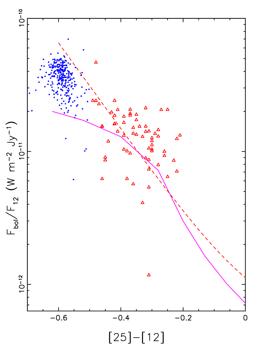
We utilize a bolometric correction derived from the models described in IE95 and computed by the DUSTY code (Ivezić, Nenkova & Elitzur 1997). In particular, we use “warm” silicate grains from Ossenkopf, Henning & Mathis (1992), assume that stellar spectrum is a 3000 K black body, and that the highest dust temperature is 500 K. These values provide best agreement with the data discussed by Knauer, Ivezić & Knapp (2001), and shown as symbols in Figure 5. For comparison, we show the bolometric correction determined by van der Veen & Breukers (1989), for a different sample of AGB stars, as the dashed line.
For negligible optical depths ([25]-[12] -0.6) the bolometric correction has the value corresponding to the input stellar spectrum. This value varies with the stellar temperature as T-3 because the IRAS wavelengths are in the Rayleigh-Jeans domain. As the optical depth increases, the SED is shifted towards longer wavelengths, the ratio of the flux and bolometric flux increases (i.e. BC decreases), and the [25]-[12] color becomes redder. Note that for a given the corresponding bolometric flux decreases as the [25]-[12] color becomes redder. The best-fit value for the highest dust temperature is about 200 K lower than usually assumed when modeling the SEDs of AGB stars. However, this low value is in agreement with Marengo, Ivezić & Knapp (2001) who show that AGB stars (with silicate dust) showing semi-regular variability require models with somewhat lower dust temperatures (300 K) than stars exhibiting Mira-type variability (750 K).
We conclude that it is possible to use IR bolometric correction for AGB stars to estimate their bolometric fluxes from IRAS and fluxes, albeit with an uncertainty up to a factor of 2. We show below that the actual uncertainty in derived bolometric fluxes seems not larger than 50%.
3.2 Determination of
By assuming that all AGB stars have the same luminosity, , and adopting a model-derived bolometric correction, the distance to each star is estimated from
| (4) |
The characteristic luminosity, , is, of course, unconstrained in the case of an individual star without an independent distance estimate. Nevertheless, can be estimated for an ensemble of stars because the stellar distribution has a local maximum at the Galactic center, and the distance to the Galactic center is well determined (we use 8 kpc, Reid 1989).
As shown by Habing et al. (1985), “properly” color-selected IRAS point sources clearly outline the Galactic disk and the bulge. This observation unambiguously indicates that IRAS observed AGB stars as far as the Galactic bulge; however, it is not clear what is the limiting distance to which IRAS detected AGB stars. The incompleteness effects close to the faint sensitivity limit may bias the estimate of .
We examined this limiting distance by a method that does not depend significantly on the sample completeness near the faint cutoff. We compare the counts ratio of stars seen directly towards the bulge, and disk stars (both selected by applying angular masks, see below) selected from narrow color and flux bins. Since both subsamples have the same observed flux, they are affected by incompleteness in a similar way. Similarly to the number counts, the number counts ratio of the two subsamples is also expected to show a local maximum corresponding to stars 8 kpc away. Thus, finding the flux–color bin which maximizes the bulge-to-disk counts ratio determines the bolometric flux of stars at the Galactic center, and consequently . The power of the method stems from the fact that the incompleteness effects nearly cancel out because a ratio of counts is taken.
The candidate bulge stars are selected as those within a circle coinciding with the Galactic center and radius of 10∘, except those with that are excluded because of confusion. The mask for the disk star sample is defined by and .
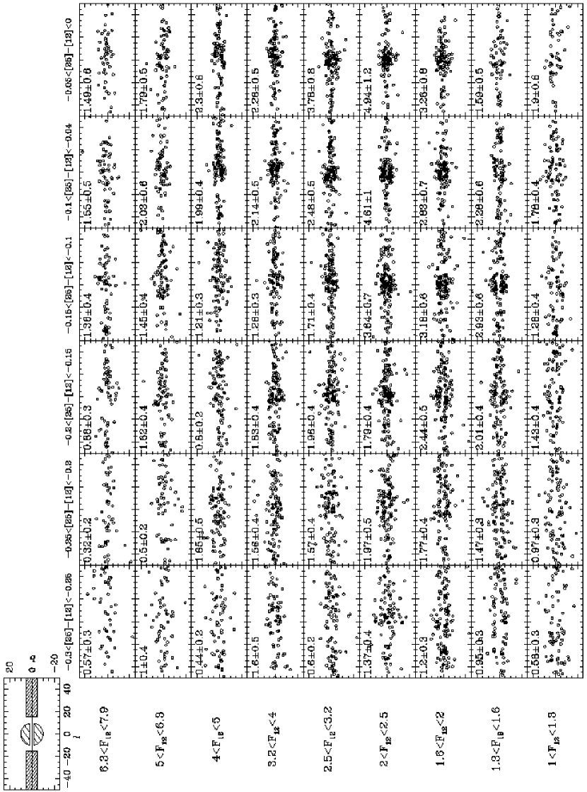
We define 60 bins555The largest distance at which an AGB star could be observed is strongly color dependent because the relationship between their characteristic luminosity, , and observed flux, , includes the color-dependent bolometric correction. For example, for = 3,500 L⊙ and = 1 Jy, stars with [25]-[12]= 0 can be seen to 14 kpc, while stars with [25]-[12]= -0.4 only to 3 kpc. This effect mandates that the analysis is performed for color ranges sufficiently narrow that the bolometric correction is approximately constant. Given the sample size and the behavior of the bolometric correction, we find that 0.05 is a good choice for the color bin size. in the vs. [25]-[12] plane, and for each determine the bulge-to-disk star count ratio (the color is limited to because bluer stars are not detected all the way to Galactic center, see below). Figure 6 shows the angular distribution of stars in these bins. The bulge and disk masks are shown in the upper left corner. It is evident that the count ratio varies greatly among the bins, and has values indicating both bulge detection () and non-detection (). For each color bin there is a local maximum of the count ratio corresponding to the stars at the Galactic center. The count ratio decreases for fainter flux because stars in those bins are behind the Galactic center.
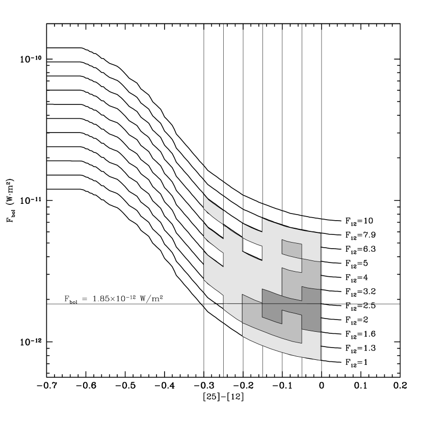
The behavior of the bulge-to-disk count ratio is easier to discern if shown in the vs. [25]-[12] plane. Figure 7 displays information similar to Figure 6, except now the counts ratio is shown by different shades: the darkest for , medium for 2 to 3, and the lightest for 1 to 2 (the bin boundaries are not rectangular any more because is used instead of ). The highest contrast is obtained for bins with [25]-[12] -0.2 and for = Wm-2. In principle, the highest contrast for each color bin should be obtained at the same value of . As evident from the figure, the bluer bins appear to imply an larger by about a factor of 2. However, the blue bins corresponding to = Wm-2 have very close to the sample completeness limit at 1 Jy: so close to the sample faint limit that even the “counts ratio” method falls apart, and the apparent bias in for blue bins cannot be interpreted as a real effect. We adopt = 1.9 Wm-2 as the bolometric flux of an AGB star at the Galactic center, implying = 3,500 L⊙ for a distance to the Galactic center of 8 kpc. This value could be uncertain by as much as a factor of 2, and we estimate its probable uncertainty below.
3.3 Optimal Bulge Selection
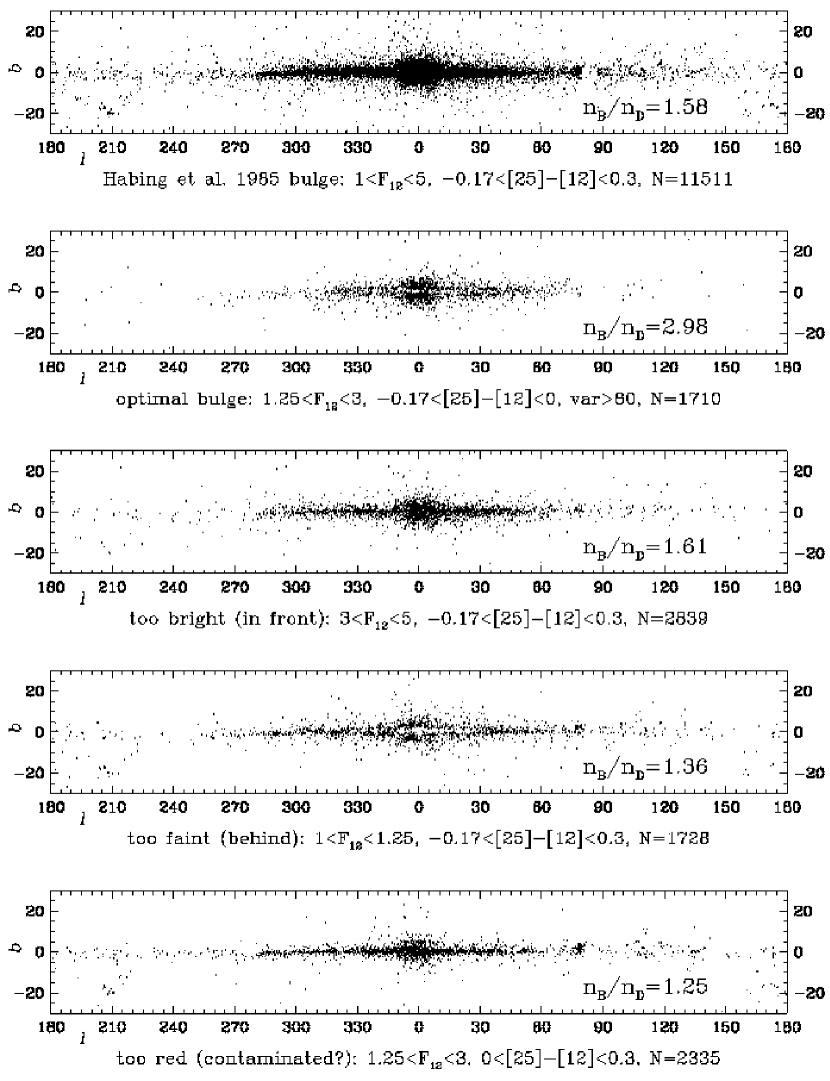
Based on the above discussion, in particular on the results presented in Figure 6, we can optimize the bulge selection criteria to minimize contamination. In essence, the vs. plane is mapped onto the distance–color plane, and requiring a distance range of e.g. 7–9 kpc simply means defining a corresponding region in the vs. plane (or, equivalently, the vs. [25]-[12] plane). We find that selecting stars with 1.25 /Jy 3.0 and [25]-[12] 0.0 produces a bulge-to-disk contrast ratio of 3. While this is lower than the maximal possible ratio (e.g. 5 for 2 /Jy 2.5 and [25]-[12] 0, see Figure 6.) the relaxed criteria produce a much larger sample (1,710 instead of 231 stars) The bulge-to-disk contrast ratio of 3 is still larger than the ratio obtained by following the prescription from Habing et al. (1985) which produces a contrast of 1.6 (albeit with a much larger sample). The angular distributions of stars selected by these two criteria are compared in the two top panels in Figure 8.
One of the reasons why the above selection produces a larger bulge-to-disk contrast than the Habing et al. sample is that their sample contains disk stars which are in front of the bulge and behind the bulge, but are observed towards the bulge. The results from Figure 6 can be used to select such stars, too. The third and the fourth panels in Figure 8 show the angular distribution of stars in front of the bulge and behind the bulge, selected from the Habing et al. sample. Another reason for the lower contrast is that their sample is probably contaminated by non-AGB stars. This contamination would be large for [25]-[12]0, and the bottom panel in Figure 8 shows the angular distribution of such stars. Their bulge-to-disk count ratio is only 1.25.
3.4 Determination of the Width of the Luminosity Function
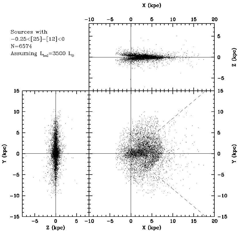
With the assumption of a constant luminosity of 3,500 L⊙, and with the bolometric correction shown in Figure 5, it is straightforward to calculate the distance for each star by using eq. 4. We assume that the extinction is 0.030 mag/kpc at 12 m and 0.015 mag/kpc at 25 m, resulting in corrections for stars at the Galactic center of 25% for the flux and for the color. In order to minimize incompleteness effects, we require 1 Jy. This is the faintest flux limit which still allows the detection of stars at the Galactic center, and results in a sample of 9,926 stars. This limit also guarantees that the sample is not affected by the IRAS faint limit at 25 m. In order to visualize the dependence of the galactic distribution of AGB stars on their [25]-[12] color, we divide the sample into the “blue” subsample with [25]-[12] (3,352 stars), and the “red” subsample with [25]-[12] (6,574 stars).
Figure 9 shows the three Cartesian projections of the galactic distribution of stars in the red subsample. The X-Y and X-Z panels indicate that the sample extends beyond the Galactic center. It is visible in the X-Z panel (upper right) that the limiting distance for stars beyond the Galactic center depends on the height above the Galactic plane. Stars close to the plane are observed through the bulge, and these lines of sight have a somewhat higher faint cutoff due to the source confusion (this effect is not caused by interstellar extinction).
The stars appear to trace out a bar-like structure of length 5 kpc pointing towards the Sun, but this is an artifact of the assumption that all stars have the same luminosity. Since the true luminosity function must have a finite width, we can estimate this width by assuming a spherical bulge.
By analyzing the counts of stars in two strips 2 kpc wide parallel to X and Y axes, we find that the equivalent Gaussian width of the start count histogram along the X axis is between 1.5 and 2.5 times as large as along the Y axis (1.2–2.0 kpc vs. 0.8 kpc). The histogram width along the X axis is harder to measure than the width along the Y axis because it is not fully symmetric around the X=0 due to the incompleteness effects behind the Galactic center. We conservatively adopt 2 kpc for the effective widening of the stellar distribution due to a finite width of the luminosity function, which implies that the scatter (the equivalent Gaussian width) of luminosity about the mean value is about a factor of 2. In other words, the majority of stars (66%) have their bolometric luminosity between 2000 L⊙ and 7000 L⊙. The assumption that all stars have the same luminosity smears their distribution such that fine details cannot be recovered.
Figure 10 shows the galactic distribution of stars in the blue subsample. For the same bolometric flux these stars have fainter IRAS fluxes than stars in the red subsample, and consequently a shorter limiting distance. As evident from the figure, these stars are not observed all the way to the Galactic center.

3.5 Analysis of the Galactic Distribution of AGB Stars
The Galactic distribution of AGB stars (using the luminosity function discussed above, = 3,500 L⊙) in Figures 9 and 10 shows jumps in the number density along the lines of sight defined by and . Both features are data artifacts. The first jump happens at the intersection of the IRAS missing data region with the galactic plane (the so-called 5∘ gap, see the IRAS Explanatory Supplement, Section III.D). The other jump at only shows up after the variability cut (). This feature, as well as other more subtle structures, is a sampling effect because in this region the source density is high and the survey strategy produced extra scans at time intervals suitable for detecting variability.
In order to minimize these effects, and to study a well-defined volume, we further limit the sample to a wedge starting at the Galactic center, symmetric around the X axis, and with an opening angle of 80∘. Its boundaries are shown by dashed lines in Figures 9 and 10. This constraint leaves 6,804 stars in the sample. While the applied restriction does not completely remove these features, it allows for a robust determination of the source distribution inside the solar circle and several kpc beyond it. However, around kpc any local features in the number density should be treated with caution. These two instrumental effects should not produce any bias in the direction, and are presumably not dependent on color.
3.6 The Non-parametric Estimates
The sample remaining after all selection cuts is still large enough to explicitly test the hypothesis that the Galactic distribution of AGB stars is separable in galactocentric distance, , and distance from the galactic plane, . If so, then the vertical () distributions in different radial () bins should be statistically indistinguishable (apart from the normalization factor). We also separate the stars by color into several subsamples in order to constrain the relationship between the color and Galactic distribution.
3.6.1 The Vertical Distribution
Figure 11 displays the distributions, shown as histograms with error bars, for 3 color subsamples (the [25]-[12] color in the ranges to , to , and to 0), and in three radial ranges (2-5 kpc, 5-8 kpc, and 8-12), starting with the top left panel. The small numbers show the number of stars in each bin (these counts are not corrected for the selection efficiency of 35%, see Sections 2.2 and 3.8). Since all histograms are well described by an exponential function,
| (5) |
we determine its scale height, , by fitting the counts for kpc. The number of stars in each subsample (N) and the best-fit scale heights are shown in each panel. The scale heights vary from 226 pc to 381 pc, with marginal evidence (3) that the scale height decreases with the [25]-[12] color. While a 3 effect may appear significant, we emphasize that the error bars are simply based on Poisson statistics, and do not include any systematic effects. A similar level of significance is obtained for the correlation between the best-fit scale height and the radial direction, where the last radial bin appears to have a somewhat larger scale height (as in e.g. a flared disk).

To test further whether the data strongly support these correlations, we determine the best-fit scale height for the whole sample, i.e. without the radial and color binning, and compare it to each subsample. The bottom right panel in Figure 11 shows the distribution for the whole sample as a histogram, and the best exponential fit by a thin solid line. The same exponential fit (for the whole sample) is then compared to each subsample in other three panels, and shown as a thin solid line. We include only points with kpc where the signal-to-noise ratio is the highest, and use the same weight for all points. As evident, the best-fit scale height of 28610 pc is not obviously inconsistent with the distribution of each subsample. While formally the per degree of freedom is somewhat larger than 1, the unknown systematic errors may account for this discrepancy. We conclude that there is no compelling evidence that the scale height depends significantly on the [25]-[12] color or the galactocentric distance.
The histogram shown in bottom right panel of Figure 11 is systematically above the best-fit exponential for kpc. This excess of counts appears consistent with the thick disk proposed by Gilmore and Reid (1983). However, this discrepancy has no statistical significance; the number of stars in all radial bins with kpc is 101, or about 1.4% of the total number of stars, comparable to the estimated 3% sample contamination by non-AGB stars (see Section 2.2). Such contaminants are dominated by stars with luminosity much smaller than the adopted AGB luminosity (3,500 L⊙). While there is growing support for the thick disk (e.g. Chen et al. 2000, and references therein), its existence is not required by the IRAS counts of AGB star candidates.
The dashed and dotted lines in bottom right panel of Figure 11 show two fits of the function. This function was proposed by Habing (1988) to be a better description of the distribution of AGB stars than a simple exponential function, and utilized to model the IRAS counts. The dashed line is a best-fit which reproduces the observed counts at . However, it falls off too fast for kpc. The dotted line produces a good fit (to the exponential best fit) for large , but it significantly underestimates the counts for = 0. We conclude that a simple exponential function is a much better description of the distribution of selected AGB star candidates than function for kpc. This conclusion is in agreement with Kent et al. (1991) who analyzed a 2.4 m map of the northern Galactic plane.
3.6.2 The Radial Distribution
The radial distribution of selected AGB candidates is shown in Figure 12. The first five panels, starting in the upper left corner, show the histograms for subsamples binned by the [25]-[12] color. As was already evident in Figure 10, the blue subsamples ([25]-[12] -0.3) do not extend all the way to the Galactic center.
The decrease of number density for 5 kpc seems consistent with an exponential fall-off, and each panel displays the best-fit scale length obtained for points with kpc (except for the bluest bin where the limit is kpc). The corresponding fit is shown by a straight line. The number of stars in each color-selected subsample is also shown in each panel. Note that there are no obvious jumps in the counts at 8 kpc, indicating that selecting the stars within the wedge described in the previous section removes the instrumental effects seen in Figures 9 and 10.
The best-fit scale lengths span the range from 1.2 kpc to 1.8 kpc, with a typical uncertainty of 0.1 kpc, and the mean value of 1.44 kpc. The bottom right panel shows the histogram for the whole sample (i.e. without the color binning); its best-fit scale length is 1.60.07 kpc, consistent with the above mean value.
The counts of stars in the red subsamples ([25]-[12] ) increase towards the Galactic center for 3-4 kpc. This increase is caused by the bulge contribution. We do not attempt to fit any analytic function because the resulting fit would be strongly affected by the errors in the adopted luminosity function; that is, the detailed dependence of the counts for kpc cannot be determined. Nevertheless, based on the counts for the subsample with [25]-[12], it appears that the disk contribution for the inner 45 kpc may be much flatter than its exponential fall-off inferred for larger . Based on the analysis presented in Section 3.2, the bulge contributes at least 3 times as many stars as the disk for = 0. This implies that the disk contribution is roughly constant within the inner 5 kpc. The counts for the reddest subsample are also consistent with this conclusion.


3.7 A Simple Model for the Galactic Distribution of AGB Stars
The galactic distribution of AGB stars determined in the previous section is only marginally inconsistent with a universal, color-independent function which appears separable in and . The distribution is well described by an exponential function with the scale height of 290 pc. The distribution has an exponential fall-off with the scale length of 1.6 kpc for 5 kpc. Within the inner 5 kpc, the counts can be described by a flat component due to the disk, and a bulge component which increases towards the Galactic center.
These results do not vary strongly with the [25]-[12] color. To illustrate this further, the three panels in Figure 13 show the dependence of best-fit scale height, scale length and the number density on color. This figure can be considered as a summary of results presented in Figures 11 and 12. The error bars are formal uncertainties of the fits and do not include the contributions from the sample contamination and various incompleteness effects. Because these contributions cannot be easily quantified, the displayed results may be interpreted in two different ways.
Formally, it seems that both the scale height and the scale length decrease with [25]-[12] color. Since the scale height decreases with the stellar mass (e.g. Allen 1973), this is consistent with the hypothesis that the mass-loss rate (which by and large controls the [25]-[12] color, see the next section) increases with stellar mass (see e.g. Habing 1996). The dependence of the scale length on color, if real, implies that the high-mass stars are more concentrated towards the Galactic center than the low-mass stars. Such a conclusion would be in agreement with the studies of star formation inside and outside the solar circle (Wouterloot et al. 1995, Casassus et al. 2000).
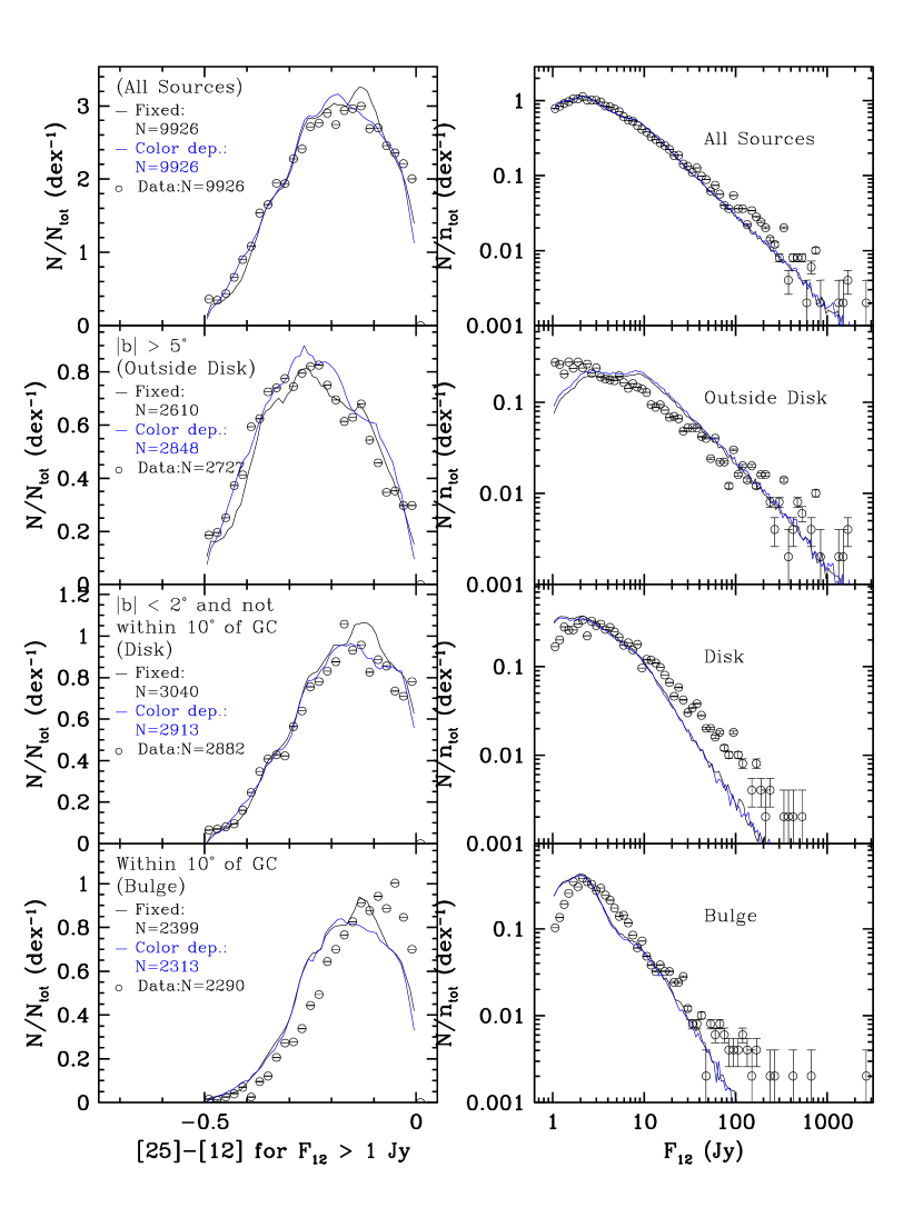
On the other hand, the statistical significance of the possible correlation between the galactic distribution of AGB stars and their [25]-[12] color is small. Since there are additional unknown systematic errors, a simple universal description of the galactic distribution cannot be strongly ruled out. Such a simple description of the distribution of AGB stars, if able to reproduce the data, would be of great value for modeling the Galaxy, as well as for modeling other galaxies. In order to estimate how well this model would describe the IRAS data we perform the following test. We assume a color-independent Galactic distribution of AGB stars as described at the beginning of this section. The bulge is assumed to follow an exponential profile with a scale length of 0.8 kpc (the precise form of the bulge profile is not important since it is not well constrained by the data) with the bulge-to-disk number ratio of 2 at = 0. Utilizing the constant luminosity =3,500 L⊙, we generate the model number counts as a function of position on the sky, the flux and the [25]-[12] color for 100 randomly generated samples. The counts depend on the color despite the color-independent distribution of stars because of the color-dependent limiting distance. The discrepancy between this model and the data illustrates the significance of the deviations from the simplified model (this test, of course, does not reveal systematic errors, as e.g. the sample contamination).
Figure 14 is reminiscent of Figure 1 and shows the comparison of the data and the simplified model. The data are shown as squares with Poisson error bars, and the model results are shown by lines. The overall normalization of the model is determined by requiring the same total number of sources as in the data sample. The completeness function at the faint end is determined by requiring the agreement between the data and model counts for the whole sample (that is, the data and the model are forced to agree in the top right panel). The real test of the model lies in the remaining panels where the data and the model are compared for different lines of sight without further model adjustments. The overall features in the color and flux distributions are reproduced fairly well, although there are some formally significant disagreements. While these disagreements illustrate the errors introduced by applying the simplified model, they do not appear sufficient to rule it out.
3.8 The number of AGB stars in the Galaxy
The model parameters derived in the previous section can be used to approximately estimate the number of AGB stars in the Galaxy by direct integration of their number density666The number of stars selected in the 80∘ wedge, 6,591, cannot be used to directly estimate the number of AGB stars in the Galaxy (by multiplying by 360/80) because the blue stars are not observed all the way to the Galactic center.. The resulting simplified model for the number density of AGB stars with [25]-[12] 0 is given by
| (6) |
where
| (7) |
for , and =1 otherwise. The radius of the inner disk part where the number density does not depend on , , is estimated to be 5.0 kpc. The scale length and the scale height are estimated as and kpc, respectively. The profile of the bulge contribution, , is not well constrained and we assume
| (8) |
with the characteristic length kpc, and the bulge-to-disk normalization .
The normalization constant can be determined from the observed local (at the solar radius) number density of AGB stars as
| (9) |
where the measured = 150 kpc-3. This value is further multiplied by a correction for the incompleteness due to selection effects estimated to be 2.9 (the variability and color selection criteria select 35% of AGB stars in the adopted color range, see Section 2.2), to yield a best estimate kpc-3. Note that the number density of AGB stars at the Galactic center is . It is hard to determine the associated uncertainty which is dominated by the unknown selection effects and the inhomogeneity of the Galactic distribution of AGB stars, but it seems that a reasonable estimate is about a factor or 2.
The integration of the above expressions shows that the number of AGB stars in the Galaxy is
| (10) |
Using the best estimates for the model parameters, we obtain = 67.7 kpc3 = 200,000. Again, this estimate is probably uncertain to within a factor of 2.
4 The time evolution of the AGB mass loss
One of the least constrained properties of AGB stars is the time evolution of their mass loss, and its dependence on fundamental stellar parameters, in particular its dependence on stellar mass. Models range from a mass loss rate that is independent of time during the AGB phase, and fully determined by the stellar mass, to a mass loss rate that increases exponentially with time, and is independent of the stellar mass (Habing 1996, and references therein).
The predictions of these models relevant for the data analyzed here pertain to the correlations between the stellar number density, color, and . Since the initial stellar mass correlates with , if the mass controls the mass-loss rate, then the [25]-[12] color, which is by and large determined by mass-loss rate, should also correlate with (i.e. the scale height should depend on color). At the same time, the color distribution would be a complicate convolution of the initial mass function and the evolutionary time scales (which also depend on the stellar mass). On the other hand, if the mass-loss rate does not depend on the stellar mass, then there should be no correlation between the scale height and color, and the distribution of colors would reflect the temporal evolution of mass-loss rate.
As shown in the middle panel in Figure 13, there is some evidence that the scale height decreases with the [25]-[12] color, as would be the case if only the high-mass stars develop large mass-loss rates. Since this result may be caused by various systematic effects, we only explore the alternative possibility that the mass-loss rate does not depend on the stellar mass, and is a universal function of time. This approach assumes that the scale height and scale length do not depend on the [25]-[12] color, and interprets the variation of the number density with color as due to temporal evolution of the mass-loss rate (see the bottom panel in Figure 13). While in principle both the variation of the scale height and the number density with color could be used to simultaneously constrain the dependence of mass-loss rate on stellar mass and time, the available data are not sufficient to derive robust conclusions in such a two-dimensional problem.
For given dust grains, the [25]-[12] color is essentially fully determined by the dust optical depth (IE95, IE97). We use a model derived relationship (the same models are used to derive the bolometric correction discussed in Section 3.1) between the [25]-[12] color and the visual optical depth, , to transform the number density vs. color relation shown in the bottom panel of Figure 13, to the number density vs. relation shown in the top panel of Figure 15.
For given luminosity, dust grains, and dust-to-gas ratio, the dust optical depth is by and large determined by the mass-loss rate (Bedijn 1987, IE95). We use a relationship derived from radiatively driven wind models with silicate dust by Elitzur & Ivezić (2001). Assuming a standard gas-to-dust mass ratio (200),
| (11) |
Note that rather than due to dust drift effects. The resulting number density vs. mass-loss rate relation is shown in the middle panel of Figure 15. The observed mass-loss rate spans the range from 10-6 M⊙/yr to 10-5 M⊙/yr (this particular range is a consequence of the analyzed range of [25]-[12] color).
The temporal behavior of the mass-loss rate is directly reflected in the observed distribution of mass-loss rate, assuming that the same function applies to all stars in the sample. For example, if the mass-loss rate increases quickly with time between two values, then most stars will be observed with a mass-loss rate closer to the low value. Following this assumption, we derive the mass-loss rate distribution shown by symbols in the bottom panel of Figure 15. The error bars are computed by assuming Poisson statistics. As evident, the increase of mass-loss rate is well described by an exponential function (i.e. log() ), and a best fit is displayed by the line.
Note that the bottom panel of Figure 15 displays the mass-loss rate as a function of , where is the time spent in the observed phase of AGB stellar evolution (not necessarily equal to the entire duration of the AGB phase due to the applied color limits). This time cannot be determined from the data analyzed here, and the only constraint we have on the mass-loss rate temporal behavior is that it is well described by an exponential function. The total number of AGB stars in the Galaxy (estimated here to be about 200,000) can be used to estimate only if the number of stars in the Galaxy that become AGB stars is known, as well as their mean lifetime. Assuming for the former, and years for the latter, reproduces the canonical AGB lifetime of years. Increasing the number of stars that undergo the AGB phase decreases the estimate of .

5 Discussion
5.1 Summary of the Results
We assume that AGB stars can be reliably selected by using the IRAS variability index and the [25]-[12] color, that their bolometric flux can be estimated from the IRAS flux and the [25]-[12] color, and that they all have the same luminosity. We estimate this luminosity to be 3,500 L⊙, and determine the distance to each star. The analysis of the resulting galactic distribution shows that it is well described by a simple function independent of color.
This is the first direct (i.e. not based on fitting the number counts) estimate of the galactic distribution of AGB stars throughout the Galaxy. It is somewhat surprising that a good description of the IRAS observations can be obtained by a model including only five free parameters: the scale height (290 pc), the radius of the inner disk where the number density does not depend on the galactocentric radius (5 kpc), the scale length (1.6 kpc) for the exponential fall-off in the outer disk, the bulge-to-disk number density ratio at the Galactic center (the bulge density is twice as large as the disk density), and the overall normalization (the local density in the disk plane at the solar radius of 100 AGB stars per kpc-3 for stars with [25]-[12] 0). The normalization is probably accurate to better than a factor of 2, and other parameters to within about 20%. The simplified model presented here implies that there are about 105 AGB stars in the Galaxy, with the uncertainty of about a factor of 2. While there exist other models that provide excellent description of IRAS counts (e.g. Wainscoat et al. 1992), they are usually much more involved that the model presented here, and often are not uniquely determined.
The final simplified model is very similar to models derived in several other studies, which are based on different methods for estimating distance. For example, Jura & Kleinmann (1992) studied the vertical scale height for 300 Mira stars with whose distance was determined from the period-luminosity relation. They determine the scale height of 240 pc for stars with periods, , longer than 300 days, in agreement with the results derived here (the period and color are correlated such that redder stars have longer periods, see Habing 1996). For stars with period shorter than 300 days they found a scale height of 500-600 pc. We do not find evidence for such an increase of the scale height for the blue subsamples. Either our selection procedure missed a significant fraction of the blue stars close to the faint end, or some stars in the sample discussed by Jura & Kleinmann had overestimated distance. Indeed, they point out that the stars in their sample with 300 days have about twice as large a velocity dispersion in the direction (55 km/s) as stars with 300 day. This may indicate that the former are contaminated by non-AGB stars.
Blommaert, van der Veen & Habing (1993) found that the number density of (red) AGB stars falls off more steeply outside the solar circle than in the inner Galaxy. This finding agrees well with the change of slope at 5 kpc evident in Figure 12. The radial scale length determined here (1.6 kpc) is at the low end of estimates in the literature (1.8–6 kpc, Kent, Dame & Fazio 1991, and references therein). However, the direct comparison is inappropriate because our value is determined for kpc, while in most other studies the assumed exponential profile extends to the Galactic center. Fitting this function to data shown in the bottom right panel in Figure 12, we obtain a scale length of 31 kpc, in agreement with recent studies. It is noteworthy that studies based on infrared data yield systematically smaller scale lengths than optical studies (Wainscoat et al. 1992, and references therein).
Jura, Yamamoto & Kleinmann (1993) found that the number ratio of stars with P 400 days and stars with 300 days P 400 days is larger at 1 kpc from the Galactic center (0.7) than locally (only 1/6). This implies that the counts ratio of blue to red AGB stars should be lower close to the Galactic center. However, the analysis presented here indicates that the counts of blue stars drop for R 2 kpc due to the IRAS flux limit. That is, we find no evidence that the ratio of red to blue AGB stars varies across the Galaxy. While this ratio may as well be different in the bulge, this is not required by the IRAS data.
5.2 Pitfalls
Of course, all of the above results critically depend on the various adopted assumptions. For example, although the estimated sample contamination is very low (3%, see section 2.2), it could be somewhat higher because the AGB nature of these stars is not positively determined for each star. Similarly, the selection does not appear biased with respect to the flux and the [25]-[12] color, but this conclusion is also based on statistical arguments. The employed model-derived bolometric correction implies that the SEDs of all AGB stars with silicate dust are self-similar. While this assumption is certainly not strictly true, it appears to be correct to within a factor of 2. A systematic bias with respect to color of the bolometric correction could produce false evidence for the dependence of the derived scale height and scale length on color. Some evidence for such dependence is borne by the data (see Sections 3.6 and 3.7, and Figure 13), but because of the bolometric correction uncertainties, it is not clear whether this effect is real.
It is obvious that the true AGB star luminosity function is not a -function; yet the shape of the distribution of stars around the Galactic center implies that the majority of stars have luminosity within a factor of 2 from the median value. The assumption that all stars have the same luminosity results in smearing of their distribution such that fine details cannot be recovered. This effect may hide some interesting features, but it does not strongly affect the overall stellar distribution.
Due to all these uncertainties, the temporal behaviour of mass loss on the AGB cannot be strongly constrained. If the dependence of the scale height and scale length is real, then the mass-loss rate increases with the stellar mass. Alternatively, if this dependence is dismissed as due to systematic effects, then the observed color distribution implies that the mass-loss rate increases exponentially with time.
5.3 Possibilities for Improvement
This work demonstrates that infrared observations of AGB stars are an excellent tool for studying the Galactic structure all the way to its center and beyond. It also reveals all the pitfalls associated with the limited data set. Fortunately, these shortcomings are solvable in principle, and the AGB stars could be utilized in a study with much greater statistical power than possible with only the IRAS data.
The reliability of AGB star selection could be improved by multi-wavelength multi-epoch observations, e.g. as those obtained by van der Veen & Habing (1990), or Whitelock, Feast & Catchpole (1991). Because of the characteristic shape of SED, and its variability properties, such observations can be used to reliably separate AGB stars from other similar sources. Additionally, the observations of various masers could be utilized as yet another signature of AGB phase (as in e.g. Jiang et al. 1991). A further important gain from the multi-wavelength observations is the ability to determine the bolometric flux directly, rather than by using a bolometric correction.
A study of the Galactic distribution of AGB stars would greatly benefit from an all-sky survey about 10 times more sensitive than IRAS. Such a survey would be capable of detecting AGB stars of all colors beyond the Galactic center, rather than only those with e.g. [25]-[12] , as with the IRAS data. By utilizing the fact that the distribution of stars is symmetric around the Galactic center, the hypothesis that the characteristic AGB star luminosity does not depend on the [25]-[12] color could be explicitly tested on a large sample of stars. Even if obtained only for the 10 area toward the Galactic center, such a survey would provide significant new constraints for the evolution of AGB stars and their Galactic distribution. We are currently investigating the possibility of using 2MASS and SIRTF surveys for such a study.
Acknowledgments
We acknowledge generous support by Princeton University, and by NASA grants NAG5-6734 and NAG5-11094 to GRK. We thank Tom Chester for clarifying the definition of IRAS variability index.
References
- [1]
- [2] Allen, C.W. 1973, Astrophysical Quantities (London: Athlone Press, 1973)
- [3] Allen, L.E., Kleinmann, S.G., & Weinberg, M.D. 1993, ApJ, 411, 188
- [4] Beichman, C.A., Neugebauer, G., Habing, H.J., Clegg, P.E. & Chester, T.J. 1985, IRAS Catalogs and Atlases (US GPO, Washington, DC)
- [5] Bedijn, P.J. 1987, A&A, 186, 136
- [6] Binney, J. & Tremaine, S. 1987, Galactic Dynamics, Princeton University Press (Princeton)
- [7] Blommaert, J.A.D.L., van der Veen, W.E.C.J. & Habing, H.J. 1993, A&A, 267, 39
- [8] Casassus, S., Bronfman, L., May, J. & Nyman, L-Å, 1999, A&A, 358, 514
- [9] Elitzur, M., & Ivezić, Ž. 2001, MNRAS, 327, 403
- [10] Habing, H.J. et al. 1985, A&A, 151, L1
- [11] Habing, H.J. 1988, A&A, 200, 40
- [12] Habing, H. 1996, A&A Rev., 7, 97
- [13] Herman, J., Burger, J.H., & Penninx, W.H. 1986, A&A, 167, 247
- [14] Gilmore, G. & Reid, N. 1983, MNRAS, 202, 1025
- [15] Ivezić, Ž., & Elitzur, M. 1995, ApJ, 445, 415 (IE95)
- [16] Ivezić, Ž., & Elitzur, M. 1997, MNRAS, 287, 799 (IE97)
- [17] Ivezić, Ž., & Elitzur, M. 2000, ApJ, 534, L96 (IE00)
- [18] Ivezić, Ž., Nenkova, M., & Elitzur, M. 1997, User Manual for DUSTY, Internal Report, University of Kentucky, accessible at http://www.pa.uky.edu/~moshe/dusty
- [19] Jiang, B.W., et al. 1997, AJ, 113, 1315
- [20] Jura, M., & Kleinmann, S.G. 1992, ApJSS, 79, 105
- [21] Jura, M., Yamamoto, A., & Kleinmann, S.G. 1993, ApJ, 413, 298
- [22] Kent, S.M., Dame, T.M., & Fazio, G. 1991, ApJ, 378, 131
- [23] Knauer, T.G., Ivezić, Ž., & Knapp, G.R. 2001, ApJ, 552, 787
- [24] Lenz, D.D., Newberg, J., Rosner, R., Richards, G.T., & Stoughton, C. 1998, ApJS, 119, 121
- [25] Marengo, M., Ivezić, Ž., & Knapp, G.R. 2001, MNRAS, 324, 1117
- [26] Mihalas, D., & Binney, J. 1981, Galactic Astronomy: Structure and Kinematics, W.H. Freeman and Company (New York)
- [27] Ossenkopf, V., Henning, Th., Mathis, J.S. 1992, A&A 261, 567
- [28] Reid, M.J. 1989, in IAU Symposium 136, The Center of the Galaxy, ed. M. Morris (Dordrecht: Kluwer Academic) p. 37
- [29] Rowan-Robinson, M. & Chester, T. 1987, ApJ, 313, 413
- [30] Rowan-Robinson, M. 1980, ApJS, 44, 403
- [31] Spitzer, L. 1978, Physical Processes in the Interstellar Medium, Wiley (New York)
- [32] van der Veen, W.E.C.J., & Habing H.J. 1988, A&A, 194, 125
- [33] van der Veen, W.E.C.J., & Habing H.J. 1990, A&A, 231, 404
- [34] van der Veen, W.E.C.J., & Breukers, R. 1989, A&A, 213, 133
- [35] van der Veen, W.E.C.J., & Rugers, M. 1989, A&A, 226, 183
- [36] Wainscoat, R.J., Cohen, M., Volk, K., Walker, H.J. & Schwartz, D.E. 1992, ApJSS, 83, 111
- [37] Walker, H.J., Cohen, M., Volk, K., Wainscoat, R.J. & Schwartz, D.E. 1989, AJ, 98, 2163
- [38] Whitelock, P., Feast, M., & Catchpole, R. 1991, MNRAS, 248, 276
- [39] Wouterloot, J.G.A., Fiegle, K., Brand, J. & Winnewisser, G., 1995, A&A, 301, 236