An adaptive filter for the PLANCK Compact Source Catalogue construction

Abstract

We develop a linear algorithm for extracting extragalactic point sources for the Compact Source Catalogue of the upcoming PLANCK mission. This algorithm is based on a simple top-hat filter in the harmonic domain with an adaptive filtering range which does not require a priori knowledge of the CMB power spectrum and the experiment parameters such as the beam size and shape nor pixel noise level.

1 Introduction

The ESA PLANCK Surveyor will produce ten all-sky high-resolution maps of the cosmic microwave background (CMB) anisotropies at 9 frequencies, from which the angular power spectrum will be derived to place constraints on the cosmological parameters. The maps produced by the PLANCK satellite, however, will not only include the CMB signal but also contain some astrophysical foreground sources arising from dust, free–free, synchrotron emission, Sunyaev-Zel’dovich effects and extragalactic point sources. It is therefore an important task to separate those foreground sources from the CMB signal. In this paper we will concentrate on the bright point sources with flux above $0.1-0.3$ Jy in connection with the Early Release Compact Source Catalogue (ERCSC) from the PLANCK mission. The main goal of the ERCSC construction is to produce such a catalogue right after the first six months of observation of the CMB sky by the PLANCK before more complicated and time consuming analysis of the CMB power spectrum, component separation and investigation of in-flight systematics. Therefore, it would be very useful to develop a fast method of the point sources extraction which needs as little information as possible about the parameters of the experiment.

In this paper, we present a fast linear algorithm for the extraction of extragalactic point sources from the CMB maps, which is a generalized amplitude-phase method of Naselsky, Novikov & Silk (2002). There have been developments of methods on point source extraction such as the high-pass filter by Tegmark and de Oliveira-Costa (1998) (hereafter TO98), Maximum–Entropy Method (MEM) by Hobson et al. (1999), and Mexican Hat Wavelet method (MHW) by Cayón et al. (2000). Here we introduce a simple top-hat filter for the extraction of point sources in the CMB maps. This method works very well without assumptions about the cosmological model, or a priori knowledge of the power spectrum of CMB and point sources.

The filter proposed by TD98 is optimal for point source extraction from the theoretical point of view, and requires the exact information about the CMB and the foregrounds power spectrum, the beam shape properties (its ellipticity and orientation), and the pixel noise level. For concrete applications, however, other methods can also be useful, which explains the succeeding discussions of other filters in the literature mentioned above and in this paper. We will compare our filter with the TD98 filter.

This paper is arranged as follows. In Section 2 we introduce the top–hat filter and elaborate the subtlety in the definition of the criterion by which the point sources are extracted. As our top–hat filtering range is adaptive, we apply in Section 3 the top–hat filter to the numerical simulated maps and estimate the filtering ranges for the PLANCK channels when the experiment parameters such as the beam size and the pixel noise level are known. We also compare our method with the theoretically optimal TD98 filter in Section 4. In Section 5 we generalize our filter to an algorithm that does not need any information about the CMB power spectrum, the beam size and the noise level. The results and discussion are in Section 6.

2 The top–hat filter

In the observed map by the PLANCK satellite the signal at pixel $i$ can be expressed as

$$d_{i}=S_{i}({\mbox{\boldmath$r$}}_{i})+n_{i}$$ (1)

where $n_{i}$ is the pixel noise, ${\mbox{\boldmath$r$}}_{i}$ correspoinds to the position of the $i$-pixel in the map and $S_{i}\equiv\Delta T/T({\mbox{\boldmath$r$}}_{i})$ includes the CMB signal and foreground contaminations, of which the relevant component to this paper is the point source contribution. Expanding $\Delta T/T$ in spherical harmonics, we have

$$\frac{\Delta T}{T}({\mbox{\boldmath$r$}}_{i})=\sum_{\ell m}B_{\ell m}a_{\ell m}Y_{\ell m}({\mbox{\boldmath$r$}}_{i}),$$ (2)

where $B_{\ell m}$ is the beam response. The main idea of our method to extract point sources is through a simple linear top–hat filter in the harmonic domain with two cut–off scales. These two scales serve to remove the influence of the lower and higher multipole parts of the total power spectrum of the signal for optimal extraction of point sources from the PLANCK maps.

In TD98 the authors introduced the ratio of the amplitude of a point source (convolved with the beam) to the variance of the total signal in the map $\sigma^{2}_{\rm tot}$, which can be denoted as

$$\overline{\Re}=\left(\frac{\langle B^{2}\otimes S^{2}\rangle}{\sigma^{2}_{\rm tot}}\right)^{1/2}.$$ (3)

Here $\langle B^{2}\otimes S^{2}\rangle=\langle(\Delta T_{\rm PS}/T)^{2}\rangle$ is the contribution from the point source relative flux $S$ to the map, $\otimes$ denotes convolution, and $B$ is the beam response, which is assumed Gaussian. They found the shape of the filter $F_{\rm TD98}$ by maximizing $F_{\rm TD98}\otimes\overline{\Re}$.

In our method we introduce a linear filter,

$${\cal F}_{\rm TH}(\ell_{\min},\ell_{\max})=\Theta(\ell-\ell_{\min})\Theta(\ell_{\max}-\ell),$$ (4)

where $\Theta$ is the Heaviside step function, i.e., $\Theta(x)=0$ for $x\leq 0$, and $\Theta(x)=1$ for $x>0$. $(\ell_{\min},\ell_{\max})$ is the filtering range of ${\cal F}_{\rm TH}$. This filter has a top–hat shape in the harmonic domain with two characteristic scales $\ell_{\min}$ and $\ell_{\max}$, both of which are functions of the antenna beam shape, the power spectrum of the CMB, the power spectra of all kinds of foregrounds and pixel noise, and possible systematic features. When these parameters are known, we can find $\ell_{\min}$ and $\ell_{\max}$ through maximizing $F_{\rm TH}\otimes R$ for each frequency channel of the PLANCK mission. Here $F_{\rm TH}$ is the filter in Eq. (4) in the real domain and $R$ is the resultant relative flux,

$$R=\Re-\nu_{\min},$$ (5)

where $\Re=(B\otimes S)/\sigma_{\rm tot}$ and $-\nu_{\min}$ is defined by $-\nu_{\min}\sigma_{\rm in}$ being the amplitude of the deepest minimum in the map, with $\sigma_{\rm in}$ the square root of the variance of the pre-filtered map.

Note that there is a subtle difference between the TD98 filtering and the top-hat optimization algorithm in the definition of the criterion by which the point sources are extracted. In order to obtain the filter shape, the TD98 filter is defined by maximizing the $\overline{\Re}$ ratio in their theoretical derivation whereas the top–hat filter is defined by maximizing the $R=\Re-\nu_{\min}$ ratio. According to the prediction of bright point source contamination in the Low Frequency Instrument (LFI) frequency range of the PLANCK mission [Toffolatti et al. 1998], point sources with flux above $0.1-0.5$ Jy are rare events in a $10^{\circ}\times 10^{\circ}$ patch of the sky. For the 30 GHz frequency channel, for example, the estimated number density of point sources is $\sim$0.3-1 source for each $10^{\circ}\times 10^{\circ}$ patch. Thus each bright point source is a peculiar peak in the $\Delta T/T$ map and the observed amplitude of the point source in the map is a combination of the point source contribution itself (which is not known), the signal from the CMB plus foregrounds convolved with beam response, and pixel noise contribution in the pixel containing the point source signal. As is mentioned in TD98, in order to extract point sources from the filtered map it is necessary to introduce a criterion to screen point sources from the ‘noise’. It is the so–called $5\sigma_{\rm f}$ criterion, which means that the peaks in the filtered map with amplitudes above $5\sigma_{\rm f}$ threshold are identified as point sources, $\sigma_{\rm f}$ being the square root of the variance of the filtered map. The amplitude of each filtered peak above $5\sigma_{\rm f}$, however, is the combination of the amplitude of the point source and the filtered ‘noise’. Therefore, generally speaking, the final (filtered) signal around the peak area with the amplitude around $5\sigma_{\rm f}$ is sensitive to the actual realization of the pre-filtered ‘noise’, which can either increase or decrease the point source amplitude depending on initial realization of the ‘noise’ signal. This is the reason why the TD98 filter can distinguish mean point source contribution from the map. In our method for the construction of the filter we consider the worst case, i.e., when the point source is at the position of the deepest minimum $-\nu_{\min}\sigma_{\rm in}$ of the signal in the map.

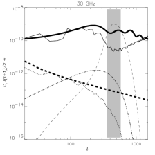
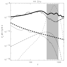
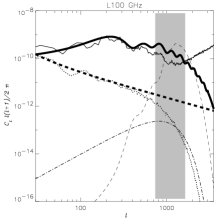
Figure 1: The angular power spectra and the optimal filtering range for the LFI channels. The thick curve is the theoretical CMB power spectrum. The thick dash line is the theoretical dust emission power spectrum, which is assumed $\propto\ell^{-3}$. The solid curve represents the beam–convolved total map, which includes dust emission (dotted line) and pixel noise. The dash–dot line is the power spectrum of the beam–convolved point source with initial amplitude $3\sigma_{\rm in}$, where $\sigma_{\rm in}$ is the square root of the variance of the pre-filtered map. The shaded area shows the optimal top–hat filtering range for the channel. For comparison, the long dash line shows the shape of the TD98 high-pass filter, which is scaled to fit into the figure.

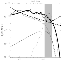
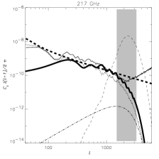
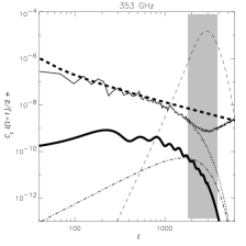
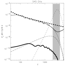
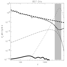
Figure 2: The angular power spectra and the optimal filtering range for the HFI channels. The notations are the same as Fig. 1.

We would like to point out the significance of the two characteristic scales $\ell_{\min}$ and $\ell_{\max}$ on enhancing the ratio of the point source flux to the $\sigma_{\rm f}$ of the filtered map. There are two main features on the total power spectrum $C_{\ell}^{\rm tot}$ from the map as shown in Fig. 1 and Fig. 2. On the low multipole end, there are the CMB itself which has the standard characteristic of $C_{\ell}\propto\ell^{-2}$ with a Harrison-Zel’dovich power spectrum from adiabatic perturbation, together with the so–called low multipole tail from the foregrounds such as dust emission, free–free and synchrotron emission. Thus the scale $\ell_{\min}$ of the top–hat filter cuts off this low multipole part of the total power spectrum $C_{\ell}^{\rm tot}$. For the high multipole end, on the other hand, the most dominant component in $C_{\ell}^{\rm tot}$ is the pixel noise. The corresponding scale $\ell_{\max}$ is therefore crucial in cutting down the pixel noise contribution in the filtered map, hence decreasing $\sigma_{\rm f}$.

The top–hat filter aims to suppress the low multipole tail and the pixel noise contribution so as to minimize the $\sigma_{\rm f}$. At the same time, it retains the part of $C_{\ell}^{\rm tot}$ that is most modified by the beam response (see the shaded area of each panel in both Fig. 1 and Fig. 2). This means that, instead of the theoretically optimal TD98 filter which needs some preliminary and detailed information about the power spectra of the PLANCK map components and corresponding beam response, the top–hat filter has the simplest shape that transforms the uncertainties of the parameters to the scales of the cut-off $(\ell_{\min},\ell_{\max})$.

In constructing the top-hat filter for a specific frequency channel, we have to estimate the two cut–off scales when the experimental parameters such as the beam size and the pixel noise level are known. To do so, we choose the deepest minimum of the ‘noise’ as the position of the point source (hence the expression of Eq. (5)) and optimize the cut-off scales $(\ell_{\min},\ell_{\max})$ exactly from such worst realization of the point source signal and ‘noise’. The filter with the filtering range obtained by the optimization of the signal $S_{\rm f}$ (point source) to the ‘noise’ $(N_{\rm f})$ ratio for the filtered map in the worst case under the condition $S_{\rm f}/N_{\rm f}\rightarrow\max$ allows us to detect all point sources with the same flux (and above) at any other different locations of the map.

Frequency	$\sigma_{\rm CMB}$	$\sigma_{\rm dust}$	$\sigma_{\rm noise}$	FWHM	Pixel size	Simulation size
(GHz)	($10^{-5}$)	( $10^{-5}$)	$(10^{-5})$	(arcmin)	(arcmin)	(squared area)
857	4.47	155700.	2221.11	5.0	1.5	$12.8^{\circ}$
545	4.47	1220.0	48.951	5.0	1.5	$12.8^{\circ}$
353	4.48	65.1	4.795	5.0	1.5	$12.8^{\circ}$
217	4.43	8.52	1.578	5.5	1.5	$12.8^{\circ}$
143	4.27	2.55	1.066	8.0	1.5	$12.8^{\circ}$
100 (HFI)	4.07	1.15	0.607	10.7	3.0	$25.6^{\circ}$
100 (LFI)	4.10	1.13	1.432	10.0	3.0	$25.6^{\circ}$
70	3.88	0.558	1.681	14.0	3.0	$25.6^{\circ}$
44	3.43	0.228	0.679	23.0	6.0	$25.6^{\circ}$
30	3.03	0.114	0.880	33.0	6.0	$25.6^{\circ}$

Table 1: We produce simulated maps (CMB signals plus dust emission convolved with antenna beams plus pixel noise) by using the experimental constraints at the 10 PLANCK channels by Vielva et al. (2001). Gaussian symmetric beam shape is assumed for both the HFI and LFI channels. The 2nd, 3rd and 4th column are the rms of the CMB, dust emission, and pixel noise, respectively (in $\Delta T/T$).

3 Estimation of the filtering range

In this section we describe the technique of the filtering range $(\ell_{\min},\ell_{\max})$ estimation for the 10 maps of the PLANCK mission. The basic model of the PLANCK experiment which details the scan strategy, pixel noise properties, beam shape analysis and different kinds of the foreground contaminations is recently discussed in Mandolesi et al. (2000), Burigana et al. (1998), Bersanelli et al. (1997), and Chiang et al. (2001). In this section in order to determine the filtering range we will first assume that all the above-mentioned characteristics of the possible signals are well determined with corresponding accuracy. This condition will be relaxed in Section 5 when we introduce a more generalized algorithm for the top–hat filtering. At this stage those well–determined characteristics allow us to estimate the optimal values of the $(\ell_{\min},\ell_{\max})$ range for the top–hat filter (Eq.( 4)) and compare the efficiency of the point source extraction from the maps by applying the TD98 and the top–hat filter. Below we will use the flat sky approximation for the CMB maps without loss of generality. Moreover, Chiang et al. (2001) have shown the importance of periodic boundary condition of simulations, which is the standard part of the flat sky approximation, for descriptions of the real signal from small patches of the sky.

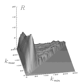
Figure 3: The display of the index $R$ as a function of $k_{\max}$ and $k_{\min}$ for the filtered map in searching for the optimal filtering range for the HFI 143 GHz channel. The amplitude of the point source is set $\Re=3.21$ and located at the deepest minimum of the initial map. The top panel shows the overall values of $R$ at different filtering ranges. The bottom panel is the contour map near the maximum. The plus sign marks the maximal $R$ and the contour line at 15.0 around the maximum covers roughly 10% of both $k_{\min}$ and $k_{\max}$. Note that the maximum in this case does not coincide with the optimal value we choose. Please see the context for details.

We produce for each PLANCK observing frequency channel a set of realizations of simulated maps using the data provided by Vielva et al. (2001). The details of the simulations are listed in Table 1. The CMB signals are created from the angular power spectrum of the $\Lambda$CDM model by Lee et al. (2001). Dust emission is simulated with power law index $-3$. The free-free and synchrotron emissions are not simulated and added to obtain the filtering range $\ell_{\min}$ and $\ell_{\max}$ in Table 2. Without adding these two parts of foreground emissions would, of course, affect the estimation of the filtering range, especially for LFI frequency channels, where the rms of both emissions are less than by one order of magnitude or comparable to that of CMB. As the free-free and synchrotron would have been assumed Gaussian, what would be modified is not the filtering range but the enhancement factor $R$. Moreover, as will become clear in Section 5, these filtering ranges serve as the initial values for the iteration scheme when we generalize the top-hat filter. The combined realization is then convolved with the corresponding antenna beam size. In this section we assume Gaussian beams $B_{k}=\exp(-k^{2}\theta^{2}/2)$, where $\theta=\mbox{FWHM}/2.355$, but a more realistic PLANCK antenna beam shape can be modelled using the method proposed by Chiang et al. (2001), which, as will be shown in Section 5, can also be tackled without difficulty.

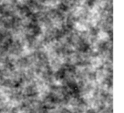
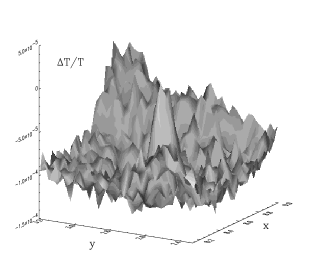
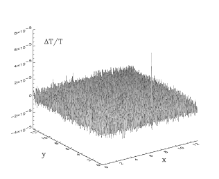
Figure 4: An illustration of the point source enhancing capability. Panel (a) shows the simulated map of HFI 143 GHz with one added beam–convolved point source of amplitude $3.21\sigma_{\rm in}$ ($\Re=3.21$). The position of the point source is circled at the lower-right quarter. Panel (b) shows the enlarged part ($x$ and $y$ axis in degrees) of beam–convolved point source of the realization which is located at the deepest minimum. We choose this frequency channel for presentation because of the small beam size and the low pixel noise level relative to the CMB signal. The shape of the beam-convolved point source is not deformed by pixel noise due to the small FWHM and the level of pixel noise. Panel (c) is the filtered map with the optimal filtering range ($k_{\min},k_{\max}$)=(42,86); the enhancement is $R=15.50$.

To estimate the $(k_{\min},k_{\max})$ filtering range, in each realization we add one beam–convolved point source with fixed amplitude $\Re=3$, which is deliberately located at the deepest minimum of the realization with beam–convolved CMB signal including foregrounds plus pixel noise. In the flat sky approximation we firstly Fourier transform the total map, then we impose the top–hat filter as in Eq. (4) with a cut–off in Fourier domain, ${\cal F}(k_{\min},k_{\max})=\Theta(|{\bf k}|-k_{\min})\Theta(k_{\max}-|{\bf k}|)$. We inverse Fourier transform the filtered Fourier ring and calculate the ratio of the peak amplitude to the $\sigma_{f}$ from the filtered map. The filtering range $(k_{\min},k_{\max})$ is determined as the one from which the maximal enhancement $R$ can be reached for the filtered map.

Figure 3 shows the surface $R$ as functions of $k_{\min}$ and $k_{\max}$ for the High Frequency Instrument (HFI) 143 GHz channel. The surface $R(k_{\min},k_{\max})$ for each frequency channel is morphologically similar, but the position for maximal $R$ can vary slightly from realization to realization owing to different lowest minimal values $-\nu_{\min}\sigma_{\rm in}$ of Eq. (5) and the effect from cosmic variance. From the contour map we can easily see that, due to the flatness around the maximum, the filtering range covers roughly 10 per cent of $k_{\min}$ and $k_{\max}$ with only a few percent of variation in enhancement. We therefore optimize the filtering range from a set of realizations for each channel. In Table 2 we show the optimal sets of the filtering range in Fourier and corresponding spherical harmonic domain for all PLANCK frequency channels.

The choice of $\Re=3$ of the initial beam–convolved point source is to make sure the enhancement $R>5$ for all the PLANCK channels. Therefore, with the top–hat filtering algorithm, we can claim that the point sources extracted will have amplitudes above $3\sigma_{\rm in}$ in the pre-filtered map. Theoretically, we can apply peak statistics to confirm that the highest point in the filtered map for the suggested filtering range should be a point source. The number of peaks above the threshold $\nu_{\rm t}$ per steradian is

$$N_{\max}(\nu_{\rm t})=\frac{\gamma^{2}}{(2\pi)^{3/2}\theta_{*}^{2}}\nu_{\rm t}\exp(-\frac{\nu_{\rm t}^{2}}{2})+$$ (6)

$$\frac{1}{4\pi\sqrt{3}\theta_{*}^{2}}\left\{1-\Phi\left[\frac{\nu_{\rm t}}{2(1-2\gamma^{2}/3)^{1/2}}\right]\right\}$$

where $\Phi$ is the error function, $\theta_{*}^{2}=2\sigma_{1}^{2}/\sigma_{2}^{2}$, and $\gamma=\sigma_{1}^{2}/\sigma_{0}\sigma_{2}$ [Bond and Efstathiou 1987]. The spectral parameters are defined as

$$\sigma_{i}^{2}=\pi\int{\ell}^{2i+1}C_{\ell}^{\rm tot}d\ell.$$ (7)

In order to find the threshold of the highest peak from the theoretical point of view, we put $A_{\rm f}N_{\max}(\nu_{\rm t})=1$, where $A_{\rm f}$ is the area of the simulation patch for each channel and $\nu_{\rm t}$ is the threshold parameter above which there is only one peak. We exclude the point source contribution from the input power spectrum $C_{\ell}^{\rm tot}$ in Eq. (7) so that the criterion for point source extraction should be set above the threshold from the calculation. The threshold before filtering $\nu_{\rm t}^{\rm i}$ and after filtering $\nu_{\rm t}^{\rm f}$ for the corresponding simulation patch of each channel are listed in Table 2. According to the $\nu_{\rm t}^{\rm f}$ values for all channels, the threshold of the highest peak for the corresponding area after filtering by the suggested range are less than $5\sigma_{\rm f}$. Hence, the $5\sigma_{\rm f}$ is an appropriate criterion for point source extraction.

Figure 4 illustrates an example of point source enhancement of a realization from the HFI 143 GHz channel. Panel  (a) shows the simulated map with one added point source of $\Re=3.21$, i.e., the amplitude of the beam–convolved point source is $3.21\;\sigma_{\rm in}$. In panel (b) we display the detailed part of the beam–convolved point source located at the deepest minimum of the map. We specifically choose the 143 GHz channel for presentation because the beam shape carried by the point source is not much deformed by the pixel noise level. This figure shows the enhancement is related to the size of FWHM, and the level of the pixel noise against the beam-convolved CMB plus foregrounds. As shown in Fig. 1 and Fig. 2, the bending of the power spectrum by the beam response can be preserved towards high multipole modes as long as the pixel noise level is low. The less the pixel noise level, the more towards the high multipole modes the filtering range shifts in order to include the bending, hence the more low multipole power is excluded in the filtered $\sigma_{\rm f}$, resulting in higher $R$. For larger FWHM (e.g. compare the power spectrum of the single point source at 143 GHz with 353 GHz channel in Fig. 2), which nevertheless bends the total power spectrum, the filtering range has to shift towards low multipoles to keep the bending part, thus more power is included in the $\sigma_{\rm f}$, resulting in smaller $R$. Panel (c) is the filtered map after the filtering ($k_{\min},k_{\max}$) = (42,86) with enhancement $R=15.5$.

Frequency	$k_{\min}$	$k_{\max}$	$\ell_{\min}$	$\ell_{\max}$	$\nu_{\rm t}^{\rm i}$	$\nu_{\rm t}^{\rm f}$
857	90	166	2539	4673	$3.45^{*}$	4.56
545	74	146	2090	4111	$3.73^{*}$	4.50
353	64	137	1810	3859	$3.85^{*}$	4.46
217	53	116	1501	3269	$4.01^{*}$	4.41
143	42	86	1192	2427	$4.11^{*}$	4.25
100 (HFI)	68	137	960	1929	4.09	4.50
100 (LFI)	52	116	736	1634	4.31	4.39
70	40	93	566	1311	4.43	4.29
44	26	68	370	958	3.90	4.08
30	25	41	356	580	4.04	3.96

Table 2: The optimal filtering range for each PLANCK frequency channel. The multipole ranges are calculated according to the corresponding simulation sizes of the maps. As the surface of $R\equiv R(k_{\max},k_{\min})$ can vary slightly from realization to realization due to different deepest minimal value of the realizations and the effect of cosmic variance, the suggested set of filtering range can be used as the initial filtering range $(k_{\min},k_{\max})^{(0)}$ for iteration schemes. The last two columns $\nu_{\rm t}^{\rm i}$ and $\nu_{\rm t}^{\rm f}$ are, before and after filtering, the theoretical values (in terms of $\sigma$) of the threshold above which there is only one peak in the corresponding area of the simulated patch. According to $\nu_{\rm t}^{\rm f}$ from all channels, the choice of $5\sigma_{\rm f}$ is appropriate for point source extraction. The sign * in the 6th column denotes the values which are calculated from direct integration of (A1.9) in Bond & Efstathiou(1987).

We set the initial value $\Re=3$ for the estimation of the optimal filtering range $(k_{\min},k_{\max})$. For $\Re>3$, the filter with the optimal filtering range will enhance the index $R$ even more. As tabulated in Table 3, the enhancement for higher frequency channels can reach above 20, which means that with our proposed method we can extract point source amplitude much less than $3\sigma_{\rm in}$ in the pre-filtered map. We can also estimate what level of the point source amplitude at each channel can be detected by the suggested filter. In Table 3 we list the amplitudes of the point sources in terms of $\sigma_{\rm in}$ which can be filtered to reach the criterion $R=5$ with the suggested range.

Frequency	$\Re$	$R_{\rm TH}$	$R_{\rm TD98}$	$R_{\rm MTD98}$	$\Re_{R=5}$
857	2.99	56.32	64.88	66.50	0.294
545	3.01	36.52	41.51	41.42	0.542
353	3.05	27.46	30.71	30.61	0.867
217	3.12	18.85	20.05	19.98	1.21
143	3.10	14.82	15.47	15.41	1.81
100 (HFI)	3.01	11.65	12.00	11.99	1.87
100 (LFI)	2.94	6.81	6.57	6.53	2.77
70	2.91	7.36	6.82	6.68	2.41
44	3.01	7.44	7.25	7.23	2.52
30	3.02	6.91	6.35	6.34	2.84

Table 3: Comparison of the enhancing capability for different filters. We simulate a set of realizations for each frequency channel. The second column shows the initial amplitude of the beam–convolved point source. The third column $R_{\rm TH}$ is the result from the top–hat filter. The fourth column $R_{\rm TD98}$ shows the TD98 filtering and the final $R_{\rm MTD98}$ is the modified TD98 filtering. The theoretically optimal TD98 filter gives better enhancement in HFI only when the FWHM of the beam, dust and noise power spectrum are correctly modelled. The last column lists the amplitudes of the point sources in terms of the square root of the variance of the total map which can be filtered to reach above $5\sigma_{\rm f}$ by the top–hat filter.

4 Comparison with the TD98 filter

Using the top–hat filter with the optimal filtering range of $(k_{\min},k_{\max})$ we can compare its efficiency and accuracy of the point source extraction from the same realizations with the TD98 filter. The TD98 filter is expressed as

$$W_{k}=\frac{B_{k}}{C_{k}^{\rm tot}}=\frac{B_{k}}{B_{k}^{2}C_{k}+C^{\rm pix}},$$ (8)

where $B_{k}$ is the beam, $C_{k}$ is the sum of the power spectrum of the CMB and foreground components and $C^{\rm pix}$ is the pixel noise power spectrum. The shape of the TD98 filter for each channel is shown with long dash line in Fig. 1 and Fig. 2, which also targets the bending of the total power spectrum. Although the TD98 filter is theoretically optimal, the trouble is that it requires the input of the CMB, and foregrounds power spectrum and the parameters of the experiments such as the beam size and shape, and the pixel noise power spectrum. As is claimed in TD98, the different inputs of cosmological models can have 20 per cent variation in $R$. In this regard, we also compare the standard (Eq. (8)) and the modified TD98 filter, which is mentioned briefly in their paper. The modified version is that, instead of inserting any theoretical CMB power spectrum from different cosmological models and power–law foregrounds into $C_{\ell}^{\rm tot}$ in the filter ($C_{k}^{\rm tot}$ in the flat sky approximation), we can simply insert $C_{\ell}^{\rm tot}$ from the observed map itself as long as the power spectrum of the CMB is not severely modified by point sources, which is the case when we only have one point source in the simulated map. This is to compensate any fluctuations caused by cosmic variance. The bonus of this is that the modified TD98 filter does not depend on any cosmological models. In Table 3 we show from the top–hat, the TD98 and modified TD98 filter the enhancement factor of a $3\sigma_{\rm in}$ point source at the deepest minimum of the map from a set of realizations. We can see that for LFI channels, the top–hat filter performs better than both TD98 and the modified TD98 filters at the worst situation. We would like to point out that the TD98 filter is optimal when targeting the mean $R$, i.e., when a few point sources are located at both above and beneath the mean level of the map. We therefore list also in Table 4 the enhancement factor $R$ by placing one point source at a random position of a map and calculate the mean enhancement factor for a set of realizations. It is shown that the TD98 filter performs better than the top–hat filter, indicating that the top–hat filtering is $\sim$13-15% below the optimal extraction of point sources. This would transfer to roughly 7-10% loss of point source extraction compared to the TD98 filter when all the parameters are known, such as the CMB, dust power spectrum, beam properties, and the noise level.

Frequency	$R_{\rm TH}$	$R_{\rm TD98}$	$R_{\rm MTD98}$
857	55.91	65.29	66.81
143	14.54	16.92	16.90
70	7.31	8.31	8.29
30	6.94	8.24	8.21

Table 4: Comparison of the enhancing capability for the filters on point sources at random positions. Here we show two channels for both LFI and HFI. We put one point source with $\Re=3$ at a random position of a realization and calculate the mean enhancement factor $R$ from a set of realizations. The second column is the result from the top–hat filter with the suggested filtering range in Table 2. The third column $R_{\rm TD98}$ shows the TD98 filtering and the final $R_{\rm MTD98}$ is the modified TD98 filtering.

To compare from the theoretical point of view the enhancement factor in details between these two filters for a single point source, we need the information of the location and amplitude of the point source. Specifically when we place one point source at the deepest minimum, this situation favours the top–hat filter, as the top–hat filter is ‘designed’ for this situation and similar situations such as other local minima. Also the amplitude of the point source is crucial in the enhancement factor $R$. Though from Table 3 for the HFI channels the $R$ from TD98 filter is higher, it does become smaller than that from the top–hat filter when the point source amplitude is significantly smaller than $3\sigma_{\rm in}$.

5 Generalization of the top–hat filter

The determination of the top–hat filtering range for each channel is sensitive to the CMB power spectrum model, pixel noise properties, beam shape and foregrounds contamination. However, for the proposed ERCSC construction it is absolutely necessary to simplify the method of the point source detection from the map, using general characteristics of the ‘noise’ and point sources only. We would like to point out specifically that the point source filter with adaptive range and a fixed shape, such as the top–hat filter is a much simpler way to define such kind of filters. As the concept of the top–hat and the TD98 filter to extract point sources takes advantage of the bending on the power spectrum by the beam response and the pixel noise level, they are both useful for the regions near the ecliptic plane in the flat sky approximation, where the scans are nearly parallel without crossings (see the fig.1 of Delabrouille, Patanchon & Audit 2002). For high galactic latitude scans, however, the crossings of scans complicate the beam shape configuration. The effective asymmetric beam will manifest itself in the Fourier domain which is not isotropic in the Fourier ring (see the Fig.1 of Chiang et al. 2001). It is unknown whether the global beam orientation is fixed (parallel) in the scans of PLANCK. If it is not, it will have degradation effect on point source extraction from any input of fixed beam function, such as the TD98 filter and MHW method.

To tackle this problem and also to relax the condition we set earlier in Section 3 to determine the filtering range, we would like to expand the top–hat filter to a more generalized algorithm. Following Naselsky, Novikov & Silk (2002), we can apply the iteration scheme for point source extraction from the map, using as the initial step of iterations the suggested $(\ell_{\min},\ell_{\max})$ parameters from Table 2. Without acquiring the exact characteristics of the experiment such as pixel noise level and beam shape and size, the initial filtering with the suggested set of $(\ell_{\min},\ell_{\max})$ may not result in maximal enhancement for that specific realization. We can, however, always find the highest peak in the filtered map after the first top–hat filtering. There are two possibilities for the value of the amplitude of such peak. If we choose the criterion for the point source detection as $5\sigma_{\rm f}$, it is likely that the actual value of the amplitude for the highest peak satisfies this criterion, from which we can claim we have identified a point source that can be removed easily from the map. If the highest peak is less than $5\sigma_{\rm f}$, we can make the second iteration by slightly fine–tuning the $\ell_{\min}$ and $\ell_{\max}$ parameter. For the highest peak $<5\sigma_{\rm f}$ after the first iteration, if we still cannot increase its filtered amplitude up to the criterion after fine-tuning, we can claim that it is not a point source. Of course, for higher frequency channels of HFI we can set the criterion lower than $5\sigma_{\rm f}$ as shown in Table 3, which means we can detect point sources with $\Re<3$.

The principal idea is that, with an adaptive filtering range, we can change $k_{\max}$ and $k_{\min}$ step by step to check the change of $R$ of the highest peak. In each iteration we need to compare the amplitude of the highest peak (after filtering) with the criterion for point source detection. For this algorithm, suppose that for the 100 GHz channel of HFI we put a point source with $\Re=3$ at an unknown position in the map and the pixel noise level is twice the predicted value. When we apply the filter with the suggested range, we can detect the highest point, which is less than $5\sigma_{\rm f}$. By tuning the $k_{\max}$ with fixed $k_{\min}$ to re-filter the original map, we can always find the enhancement $R$ by going through a bump along $k_{\max}$. The position of the highest peak in the filtered map is the same as the initial iteration, but with different $R$, which indicates our suggested filtering range is not optimal. Then we fix the $k_{\max}$ corresponding to the maximum $R$ of the bump, re-filtering along the $k_{\min}$ axis to find the $k_{\min}$ corresponding to the maximal $R$. Through this process we can always find the new $k_{\min}$ and $k_{\max}$ parameter which has the maximal enhancement $R$.

6 Discussions and Conclusion

We have introduced a simple and fast top–hat filter for extraction of point sources in CMB maps. As the filter cut–off range is adaptive, we can estimate it with the simulated maps when the parameters of the PLANCK channels are known.

We would like to emphasise that the main shape of the antenna beam for the PLANCK mission is close to elliptical due to optical distortions and telescope designs [Burigana et al. 2000]. The orientation of the beam, therefore, is crucial for any methods of point source extraction, which should be taken into account in order for maximal extraction of point sources. Our top–hat iteration algorithm, however, does not need this part of information and it will be even more useful if there is change of the beam shape due to the degradation effects of the mirrors during the mission.

We also perform detailed comparison of the proposed top–hat algorithm with the TD98 filter. The advantage of our method is that it is very simple, fast and does not require any detailed information about the real beam shape, the spectra of CMB and noise, and possible correlations in the pixel noise. In practice one can take the ready filter with the suggested range from Table 2 for each PLANCK frequency channel (if desirable) to improve it by the simple and fast algorithm described in Section 5. We would like to mention that the efficiency $R$ for the top–hat filter and the TD98 filter shown in Table 3 are practically the same.

References

- [Bersanelli et al. 1997] Bersanelli M., Muciaccia P.F., Natoli P., Vittorio N., Mandolesi N., 1997, A&AS, 121, 393
- [Bond and Efstathiou 1987] Bond J.R., Efstathiou G., 1987, MNRAS, 226, 655
- [Burigana et al. 1998] Burigana C., Maino D., Mandolesi N., Pierpaoli E., Bersanelli M., Danese L., Attolini M.R., 1998, A&AS, 130, 551
- [Burigana et al. 2000] Burigana, C., Natoli P., Vittorio N., Mandolesi N., Bersanelli M., 2000, preprint (astro-ph/0012273)
- [Cayón et al. 2000] Cayón L., Sanz J.L., Barreiro R.B., Martínez-González E., Vielva P., Toffolatti L., Silk J., Diego J.M. & Argüeso F., 2000, MNRAS, 315, 757
- [Chiang et al. 2001] Chiang L.-Y., Christensen P.R., Jørgensen H.E., Naselsky I.P., Naselsky P.D., Novikov D.I., Novikov I.D., 2001, A&A accepted (astro-ph/0110139)
- [Coles and Barrow 1987] Coles P., Barrow J. D., 1987, MNRAS, 228, 407
- [Delabrouille, Patanchon and Audit (2002)] Delabrouille J., Patanchon G., Audit E. 2002, MNRAS, 330, 807
- [Hobson et al. 1999] Hobson M. P., Barreiro R. B., Toffolatti L., Lasenby A.N., Sanz J.L., Jones A.W., Bouchet F.R. 1999, MNRAS, 306, 232
- [Lee et al. 2001] Lee A.T., et al. 2001, ApJ, 561, L1
- [Mandolesi et al. 2000] Mandolesi N., Bersanelli M., Burigana C., Gorski K.M., Hivon E., Maino D., Valenziano L., Villa F., White M., 2000, A&AS, 145, 323
- [Naselsky, Novikov and Silk 2002] Naselsky P., Novikov D., Silk J., 2002, ApJ, 565, 655
- [Tegmark and de Oliveira-Costa 1998] Tegmark M., de Oliveira-Costa A., 1998, ApJ, 500, 83
- [Toffolatti et al. 1998] Toffolatti L., Argueso Gomez F., de Zotti G., Mazzei P., Franceschini A., Danese L., Burigana C., 1998, MNRAS, 297, 117
- [Vielva et al. 2001] Vielva P., Martínez–González E., Cayón L., Diego J.M., Sanz J.L., Toffolatti L., 2001, MNRAS, 326, 181
- [Zabotin and Naselsky 1985] Zabotin N.A., Naselsky P., 1985, Sov. Astr., 29, 614