The power-law behaviours of angular spectra of polarized Galactic synchrotron

Abstract

We study the angular power spectra of polarized Galactic synchrotron in the range $10\mathrel{\mathchoice{\vbox{\offinterlineskip\halign{\hfil$\displaystyle#$\hfil\cr<\cr\sim\cr}}}{\vbox{\offinterlineskip\halign{\hfil$\textstyle#$\hfil\cr<\cr\sim\cr}}}{\vbox{\offinterlineskip\halign{\hfil$\scriptstyle#$\hfil\cr<\cr\sim\cr}}}{\vbox{\offinterlineskip\halign{\hfil$\scriptscriptstyle#$\hfil\cr<\cr\sim\cr}}}}l\leq 800$, at several frequencies between 0.4 and 2.7 GHz and at several Galactic latitudes up to near the North Galactic Pole. Electric- and magnetic-parity polarization spectra are found to have slopes around $\alpha_{E,B}=1.4-1.5$ in the Parkes and Effelsberg Galactic-Plane surveys, but strong local fluctuations of $\alpha_{E,B}$ are found at $|b|\simeq 10^{\circ}$ from the 1.4 GHz Effelsberg survey. The $C_{PIl}$ spectrum, which is insensitive to the polarization direction, is somewhat steeper, being $\alpha_{PI}=1.6-1.8$ for the same surveys. The low-resolution multifrequency survey of Brouw and Spoelstra (1976) shows some flattening of the spectra below 1 GHz, more intense for $C_{E,Bl}$ than for $C_{PIl}$. In no case we find evidence for really steep spectra. The extrapolation to the cosmological window shows that at 90 GHz the detection of E-mode harmonics in the cosmic background radiation should not be disturbed by synchrotron, even around $l\simeq 10$ for a reionization optical depth $\tau_{\mathrm{ri}}\mathrel{\mathchoice{\vbox{\offinterlineskip\halign{\hfil$\displaystyle#$\hfil\cr>\cr\sim\cr}}}{\vbox{\offinterlineskip\halign{\hfil$\textstyle#$\hfil\cr>\cr\sim\cr}}}{\vbox{\offinterlineskip\halign{\hfil$\scriptstyle#$\hfil\cr>\cr\sim\cr}}}{\vbox{\offinterlineskip\halign{\hfil$\scriptscriptstyle#$\hfil\cr>\cr\sim\cr}}}}0.05$.

, , , , , ,

1 Introduction

Angular power spectra (henceforth, APS) of the Galactic synchrotron polarized radiation are raising up an increasing attention in these years. The first study, based on the Parkes 2.4 GHz survey (Duncan et al. 1997, hereafter D97), was due to Tucci et al. (2000), and other papers appeared shortly after (Baccigalupi et al., 2001a; Giardino et al. 2001). The main motivation for these works was the need for an angular-scale–dependent separation of the cosmic microwave background (CMB) signal from the polarized radio foreground; in fact the first work on the APS of a polarized Galactic foreground (Prunet et al. 1998) modelled thermal dust emission in view of the scenario to be met by Planck HFI at 143-217 GHz. CMB polarization is essential in order to remove degeneracies between important cosmological parameters (Zaldarriaga et al. 1997), but the cosmological window (the region in the frequency–angular-scale plane where the cosmological signal is stronger than foregrounds) is narrower for polarization than for anisotropy. A careful study of Galactic contamination versus angular scale is thereby necessary. The study of synchrotron APS may also be important because of its bearing on the knowledge of Galactic structure, and in particular of the transverse magnetic field in emission regions and the longitudinal field in compact foreground screens (Tucci et al. 2001). This point is open to future studies.

The purpose of this work is to check the generality of the APS behaviour found by Tucci et al. (2000): Electric and magnetic parity APS are governed (with reasonable approximation for $100\leq l\leq 800$) by power laws $C_{E,Bl}\propto l^{-\alpha_{E,B}}$ with $\alpha_{E,B}\simeq 1.4-1.5,$ in the portion of the Southern Galactic Plane probed by the D97 Parkes survey. Although such slopes are close to the values $\alpha_{E,B}^{\mathrm{(dust)}}\simeq 1.3-1.4$ found for thermal dust emission (Prunet et al. 1998), later work cast serious doubts on the generality of this behaviour, as far as synchrotron is concerned. For the APS of the scalar $PI\equiv\sqrt{Q^{2}+U^{2}}$ somewhat steeper spectra, with $\alpha_{PI}$ ranging from $1.7\pm 0.2$ to $1.9\pm 0.3$, are given for the Galactic Plane by Baccigalupi et al. (2001a) and Giardino et al. (2001). The former authors also find a much higher slope, $\alpha_{PI}=2.9\pm 0.2$ for $l\mathrel{\mathchoice{\vbox{\offinterlineskip\halign{\hfil$\displaystyle#$\hfil\cr<\cr\sim\cr}}}{\vbox{\offinterlineskip\halign{\hfil$\textstyle#$\hfil\cr<\cr\sim\cr}}}{\vbox{\offinterlineskip\halign{\hfil$\scriptstyle#$\hfil\cr<\cr\sim\cr}}}{\vbox{\offinterlineskip\halign{\hfil$\scriptscriptstyle#$\hfil\cr<\cr\sim\cr}}}}10^{2},$ out of the Galactic Plane from the 1.4 GHz, low-resolution survey of Brouw and Spoelstra (1976: BS76). This discrepancy would be important when evaluating the synchrotron contamination at large scales; it would thereby be rather unconfortable in view of the role of CMB polarization harmonics with $l\approx 2-20$ in the separation of effects of the primordial gravitational background from those of the secondary ionization of the cosmic medium. [This is one of the objectives of the SPOrt project, see e.g. Cortiglioni et al. (2001).] Note that the situation is not quite clear for the total intensity $I$ either: Large values $\alpha_{I}\simeq 3$ are supported by Bouchet and Gispert (1999) and Giardino et al. (2001), but $\alpha_{I}\approx 2$ follows from analysis of the Jodrell Bank 5-GHz interferometric survey by Giardino et al. (2000).

Here we extend our analysis of APS in the Galactic Plane considering the 2.7 GHz Effelsberg survey (Duncan et al. 1999: D99); further, we analyse several patches at intermediate Galactic latitudes, $\left|b\right|\leq 20^{\circ}$, from the 1.4 GHz Effelsberg survey (Uyaniker et al. 1999: U99), and finally three regions from BS76, at 5 frequencies between 408 and 1411 MHz, covering latitudes up to near the North Galactic Pole. Following Tucci et al. (2001) and thereby extending the analysis of Baccigalupi et al. (2001a), we carefully distinguish between the APS providing a fuller statistical description of the spin-2 polarization field (i.e., $C_{El}$ and $C_{Bl}$, from which $C_{Pl}=C_{El}+C_{Bl}$ is usually computed), and the $C_{PIl}$ spectrum which takes into account only the magnitude of the polarization pseudovector. This is necessary because Tucci et al. (2001) find quite significant differences between $C_{Pl}$ and $C_{PIl}$ both for a Gaussian polarization field, as predicted in the standard scenario for CMB, and for synchrotron radiation.

Our results confirm that slopes around $1.4-1.5$ in the range $100\leq l\leq 800$ are preferred on the average, in both the Northern and the Southern Galactic Plane for $C_{El}$, $C_{Bl}$ and $C_{Pl}$, although significant fluctuations around theses values are found in $10^{\circ}\times 10^{\circ}$ patches. The fluctuations however become stronger in small patches out of the Galactic Plane, so that a preferred slope should not regarded as meaningful for the U99 survey. In fact, the partial regularities that we find for polarization APS do not support the usefulness of global (i.e., full sky) $C_{E,Bl}$ for a satisfactory description of the spatial distribution of synchrotron: Local $C_{E,Bl}$ based on Fourier analysis are much more suitable to this purpose. A consistent picture, however, emerges at all of the scales we investigated. As a matter of facts, from the low-resolution BS76 survey we find moderate slopes for $l\leq 70$, at all frequencies and even near the Galactic Pole. Due to the limited range of $l$ available for the fits, we find strong correlations between fitted parameters and, as a consequence, large error bars; however there is no evidence for steep spectra, since the best values lie in the range $\alpha_{E,B}\simeq 0.5-2.0$ almost everywhere and are particularly small at frequencies where Faraday rotation is more important. For the $C_{PIl}$ spectrum, the slope fluctuations are smaller than for $C_{E,Bl}$. Our best value for $\alpha_{PI}$ is $1.6-1.8$ at all resolutions and Galactic latitudes, and all frequencies $\geq 1.4$ GHz. The difference between $C_{E,Bl}$ and $C_{PIl}$ is significant, although not large in the average. The latter quantity should thereby be confronted with $C_{PIl}^{\mathrm{(CMB)}}$, not with the $C_{E,Bl}^{\mathrm{(CMB)}}$ spectra which are popular among cosmologists, and this is properly done in the last Section of this paper.

All of the results that we provide for polarization APS should not be affected by contamination from point sources; regions with flat $C_{Il},$ on the other hand, are possibly dominated by point sources in total intensity, and are used in this paper to derive upper limits on their contribution to polarization APS, as discussed in Section 3.

2 Data analysis

2.1 Polarized synchrotron surveys

Our first high-resolution analysis of Galactic-Plane synchrotron polarization was performed on the 2.4 GHz Parkes survey (D97); this study, using twelve $10^{\circ}\times 10^{\circ}$ square patches (Tucci et al. 2000), is extended here to the 2.7 GHz Effelsberg survey (1999: D99) covering the additional Galactic longitude range $5^{\circ}\leq\ell\leq 74^{\circ}$ (see Table 1) and providing six more $10^{\circ}\times 10^{\circ}$ patches. A belt extended about 54% of the Galactic Plane is thereby covered, although with two slightly different frequencies. The FWHM resolutions are $10.4^{\prime}$ and $5.1^{\prime}$ respectively, sufficient to achieve angular scales up to $l\sim 10^{3}$. The nominal rms noise in D97 is 8 mK for total power and 5.3 mK for polarization (5.3 and 2.9 mK in some more sensitive areas), while in D99 the rms noise is 9 mK.

Table 1: Sky regions used for computation of APS

Ref.	$\nu$ (GHz)	$\mathrm{FWHM}$	Galactic latitudes	Galactic longitudes
D97	2.4	$10.4^{\prime}$	$-5^{\circ}\leq b\leq 5^{\circ}$	$-122^{\circ}\leq\ell\leq 5^{\circ}$
D99	2.7	$5.1^{\prime}$	$-5^{\circ}\leq b\leq 5^{\circ}$	$5^{\circ}\leq\ell\leq 74^{\circ}$
			$4^{\circ}\leq b\leq 20^{\circ}$	$45^{\circ}\leq\ell\leq 55^{\circ}$
			$3.5^{\circ}\leq b\leq 10^{\circ}$	$140^{\circ}\leq\ell\leq 153^{\circ}$
U99	1.4	$9.3^{\prime}$	$3.8^{\circ}\leq b\leq 15^{\circ}$	$190^{\circ}\leq\ell\leq 210^{\circ}$
			$5^{\circ}\leq b\leq 15^{\circ}$	$65^{\circ}\leq\ell\leq 95^{\circ}$
			$-15^{\circ}\leq b\leq-5^{\circ}$	$70^{\circ}\leq\ell\leq 100^{\circ}$
			$-10^{\circ}\leq b\leq 20^{\circ}$	$120^{\circ}\leq\ell\leq 180^{\circ}$
BS76	$0.41-1.4$	$2.3^{\circ}-0.6^{\circ}$	$26.5^{\circ}\leq b\leq 62.5^{\circ}$	$\ell_{\mathrm{c}}=60.5^{\circ},\Delta\psi=\pm 27^{\circ}$
			$60.5^{\circ}\leq b\leq 84.5^{\circ}$	$\ell_{\mathrm{c}}=30^{\circ},\Delta\psi=\pm 15^{\circ}$

Our study is further extended to moderate Galactic latitudes analysing the maps of the Effelsberg 1.4 GHz survey (U99), consisting of five regions fairly close to the Galactic Plane, $-15^{\circ}\leq b\leq 20^{\circ}$. The angular resolution is there $9.35^{\prime}$, and the rms noise is about 15 mK for total intensity and about 8 mK for linear polarization. The above regions having different sizes, we extracted different numbers of patches from them, namely, 1, 2, 2, 3 and 3 patches respectively, for regions corresponding to increasing row numbers in the U99 sector of Table 1. The patch size is $10^{\circ}\times 10^{\circ}$ almost everywhere (so that a portion of the first region is not used), but only $6^{\circ}\times 6^{\circ}$ in the second region.

Figure 1: The selected patches in the BS76 survey. The patches are the same at all frequencies; the dots give the locations of the original BS76 measurements at 408 MHz.

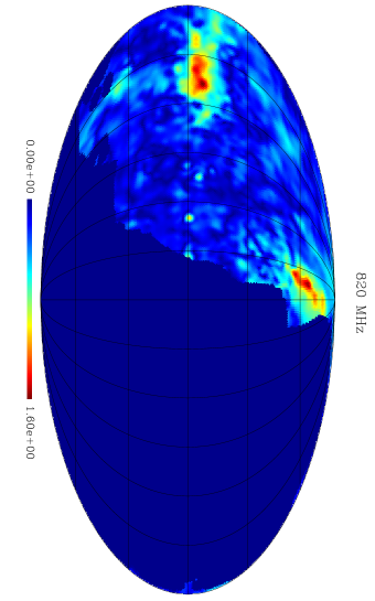
Figure 2: The total polarization ($PI$) field (in Kelvin degrees) for the BS76 survey at 820 MHz, computed applying a Gaussian smoothing with $\mathrm{FWHM}=3^{\circ}$ to the $Q$ & $U$ fields.

Finally we analysed the maps of Brouw and Spoelstra (1976: BS76) at five frequencies between 408 and 1411 MHz. The corresponding beamwidths and noise levels are summarized in Table 2. These maps cover a substantial (more than 40%) part of the sky, allowing us to compare results at quite different latitudes up to near the Galactic Pole, although with moderate resolutions. In order to get good sampling and large signal-to-noise ratios we selected three rectangular regions, whose locations are reported in the last three rows of Table 1 and in Fig. 1. As an example, we show the 820-MHz total polarization signal in Fig. 2. The BS76 maps are affected by undersampling, and the grid spacing (typically larger than the $\mathrm{FWHM}$) depends on the sky region and frequency. In the selected patches the average grid spacing is about $2^{\circ}$. To make Fourier analysis feasible we thereby constructed three new, evenly spaced grids adopting a Gaussian smoothing function with dispersion $\sigma_{\mathrm{sm}}=\mathrm{FWHM}/\sqrt{8\ln 2}$ and $\mathrm{FWHM}=3^{\circ}$. This procedure is straightforward near the Galactic Plane, where geodesics orthogonal to meridians can be identified with parallels with no appreciable errors. At high latitudes we constructed the grids projecting orthogonal geodesics, evenly spaced with $\Delta b=1.5^{\circ}$ at starting points, out of the central meridian of each patch, having longitude $\ell=\ell_{\mathrm{c}}$ as reported in the last two rows of Table 1. On such geodesics, extended respectively up to proper lengths $\Delta\psi=\pm 27^{\circ}$ and $\pm 15^{\circ}$, we picked out the centres of the Gaussian beams, with spacing $\Delta\psi^{\prime}=1.5^{\circ}$. (Since these centres do not lie on parallels, the latitude ranges in the Table refer to central longitudes $\ell_{\mathrm{c}}$.) We checked that for the chosen $\Delta\psi$ the proper distance between corresponding points on neighbour geodesics remains sufficiently close to $\Delta\psi^{\prime}$ even at the extremal longitudes $\ell=\ell_{\mathrm{c}}\pm\Delta\psi$. This in fact provides an intrinsic check for the applicability of flat-space concepts to celestial-sphere patches.

Table 2: Parameters of the BS76 survey

$\nu$ (MHz)	$\mathrm{FWHM}$ (∘)	Noise (K)
408	2.3	0.34
465	2.0	0.33
610	1.5	0.16
820	1.0	0.11
1411	0.6	0.06

2.2 Computation of angular spectra

Because of the limited sky coverages, power spectra can be suitably obtained from Fourier analysis instead of the standard spherical-harmonic approach (Seljak 1997). The estimators for the power spectra of fields can be derived by means of

$$C_{Xl}=\left[\frac{\Omega}{N_{l}\mathbf{\,}}\sum_{\stackrel{{\scriptstyle\rightarrow}}{{l}}}X(\stackrel{{\scriptstyle\rightarrow}}{{l}})X^{*}(\stackrel{{\scriptstyle\rightarrow}}{{l}})\mathbf{-}w_{X}^{-1}\right]b_{l}^{-2}\mathbf{,}$$ (1)

where $\Omega$ is the solid angle of the patch under analysis, $N_{l}$ the number of Fourier modes in the interval around $l$ chosen for averaging, $w_{X}^{-1}$ the noise contribution and $b_{l}$ the beam function. Note that $X(\stackrel{{\scriptstyle\rightarrow}}{{l}})$ is the discrete Fourier transform of the smoothed field $X(\theta_{i},\phi_{i})$, a function of the bin coordinates which can be any of the Stokes parameters $I$, $Q$ and $U$, but also (considering the electric and magnetic parity polarization) $E$ and $B$. In the small scale limit, electric and magnetic modes can in fact be given in terms of $Q$, $U$ modes by means of a simple rotation in $l$–space:

$$E(\stackrel{{\scriptstyle\rightarrow}}{{l}}) = Q(\stackrel{{\scriptstyle\rightarrow}}{{l}})\cos(2\phi_{\stackrel{{\scriptstyle\rightarrow}}{{l}}})+U(\stackrel{{\scriptstyle\rightarrow}}{{l}})\sin(2\phi_{\stackrel{{\scriptstyle\rightarrow}}{{l}}}),$$

$$B(\stackrel{{\scriptstyle\rightarrow}}{{l}}) = -Q(\stackrel{{\scriptstyle\rightarrow}}{{l}})\sin(2\phi_{\stackrel{{\scriptstyle\rightarrow}}{{l}}})+U(\stackrel{{\scriptstyle\rightarrow}}{{l}})\cos(2\phi_{\stackrel{{\scriptstyle\rightarrow}}{{l}}}).$$ (2)

Thus dealing with maps of the fields $Q$ and $U,$ we end up with $C_{El}$ and $C_{Bl}$, which are most suitable for comparison with CMB spectra. Of course one could directly use $C_{Ql}$ and $C_{Ul}$, but these spectra are not rotationally invariant. The APS describing the total power of the polarization field (taking into account spatial variations of both magnitude and direction) is

$$C_{Pl}=C_{Ql}+C_{Ul}=C_{El}+C_{Bl},\qquad l\geq 2.$$ (3)

Note the lower limit on $l$, arising from the spin-2 nature of linear polarization (namely, of the $Q$, $U$ complex). Other authors have considered the APS of the polarized intensity $PI=\sqrt{Q^{2}+U^{2}}$, which is defined for any $l\geq 0$. Equation (1) still applies with $X=PI$. The $PI$ field however does not provide a complete description of polarization, being only related to the magnitude of the polarization pseudovector. The equality $C_{PIl}=C_{Pl}$ is warranted only if the polarization angle is uniform inside all the survey area, and different spectral behaviours arise even for Gaussian random fields (Tucci et al. 2001).

In conclusion as many as 7 APS can be defined, without counting cross-correlation and circular polarization spectra. Out of these, 4 are mutually independent, and out of the latter, 3 are polarization APS.

The technique based on Eqs. (1) and (2), which has been already applied by Tucci et al. (2000) on D97 data, is fairly straightfoward for the small-size patches of high-resolution surveys. As done in that work, it is implemented here with a cosine apodization to suppress border effects, and with subtraction of mean values to suppress aliasing. However, a careful analysis is required for BS76 maps. We have already remarked in the previous Subsection that for high-latitude patches we need geodesics to identify equally spaced grids to be used in Fourier analysis; now we observe that we must also take reference frame effects into account for $Q$ and $U$ fields. Such effects are especially important for our last patch under analysis, whose border is very close to the Galactic Pole.

In particular, in order to smooth the $Q$ and $U$ fields we use the following procedure: (i) at each point within a proper distance $\chi\leq 5\sigma_{\mathrm{sm}}$ from a Gaussian beam centre, we construct the polarization vector $\stackrel{{\scriptstyle\rightarrow}}{{p}}$, (ii) we perform a parallel transport of $\stackrel{{\scriptstyle\rightarrow}}{{p}}$ to the beam centre, obtaining

$$p_{\theta}^{\mathrm{(PT)}}=p_{\theta}\cos t+p_{\phi}\sin t,\quad p_{\phi}^{\mathrm{(PT)}}=-p_{\theta}\sin t+p_{\phi}\cos t,$$ (4)

with $t=\int\cos\theta\mathrm{d}\phi,$ and (iii) from $p_{\theta,\phi}^{\mathrm{(PT)}}$we recover the parallel-transported Stokes parameters $Q^{\mathrm{(PT)}}$ and $U^{\mathrm{(PT)}}$ and apply the weight function $\exp[-\chi^{2}/(2\sigma_{\mathrm{sm}}^{2})]$ to them, obtaining the smoothed quantities

$$Q_{\mathrm{sm}}^{\mathrm{(PT)}} = \frac{\sum_{k}Q_{k}^{\mathrm{(PT)}}\exp[-\chi_{k}^{2}/(2\sigma_{\mathrm{sm}}^{2})]}{\sum_{k}\exp[-\chi_{k}^{2}/(2\sigma_{\mathrm{sm}}^{2})]},$$

$$U_{\mathrm{sm}}^{\mathrm{(PT)}} = \frac{\sum_{k}U_{k}^{\mathrm{(PT)}}\exp[-\chi_{k}^{2}/(2\sigma_{\mathrm{sm}}^{2})]}{\sum_{k}\exp[-\chi_{k}^{2}/(2\sigma_{\mathrm{sm}}^{2})]}.$$ (5)

We checked that in practice the parallel transport could be made with negligible variations on any reasonable path close to geodesics, and a very convenient approximation is $t=\cos\theta_{\mathrm{ave}}\Delta\phi$, with $\theta_{\mathrm{ave}}$ the average of polar angles at the starting and end points. The smoothed fields $Q_{\mathrm{sm}}^{\mathrm{(PT)}}$ and $U_{\mathrm{sm}}^{\mathrm{(PT)}}$ are then used in Eq. (1) for the angular spectra of BS76 maps.

3 Results

3.1 High-resolution surveys

Angular spectra for total intensity and E-parity polarization found in the Galactic Plane are shown in Fig. 3. For most of the square patches the curves are reasonably approximated by power laws,

$$C_{Xl}=A_{X}l^{-\alpha_{X}}.$$ (6)

This holds not only for $X=I$ and $E$, but also for the $B$, $Q$, $U$, and $\,P$ spectra which, having similar behaviours, are not shown in the Figure. In Table 3 we report the results of spectral fits for $X=I$, $E$ and $B$, in the range $100\leq l\leq 800$ for all of the 18 Galactic Plane patches.

Figure 3: The APS for total intensity (dotted lines) end $E$-mode polarization (solid lines), from 6 patches of the 2.7-GHz Effelsberg survey and 12 patches of the 2.4-GHz Parkes survey.

Table 3: Best-fit parameters for APS from D97 and D99 surveys

$\ell\,$(∘)†	$A_{I}$ (K${}^{2})$	$\alpha_{I}$	$A_{E}$ (K${}^{2})$	$\alpha_{E}$	$\alpha_{B}$
250	0.14$\times 10^{-3}$	0.96$\,{}_{-0.08}^{+0.12}$	0.13$\times 10^{-4}$	1.58$\,\pm$0.11	1.45$\,\pm$0.11
260	0.20$\times 10^{-2}$	1.48$\,\pm$0.12	0.96$\times 10^{-5}$	1.48$\,\pm$0.12	1.32$\,\pm$0.10
270	0.02	1.02$\,\pm$0.11	2.6$\times 10^{-3}$	1.79$\,\pm$0.12	1.25$\,\pm$0.12
280	0.48$\times 10^{-4}$	0.44$\,{}_{-0.12}^{+0.08}$	0.44$\times 10^{-4}$	1.56$\,\pm$0.12	1.78$\,\pm$0.11
290	1.8	1.43$\,\pm$0.11	0.32$\times 10^{-3}$	2.04$\,\pm$0.12	1.90$\,\pm$0.12
300	0.07	1.22$\,{}_{-0.08}^{+0.12}$	0.15$\times 10^{-4}$	1.56$\,\pm$0.12	1.88$\,\pm$0.12
310	5.1	1.89$\,\pm$0.12	$0.28\times 10^{-5}$	1.11$\,\pm$0.11	0.96$\,{}_{-0.09}^{+0.12}$
320	0.48	1.76$\,\pm$0.11	0.40$\times 10^{-4}$	1.49$\,\pm$0.11	1.40$\,\pm$0.12
330	0.21	1.46$\,\pm$0.09	0.22$\times 10^{-3}$	1.57$\,\pm$0.12	1.74$\,{}_{-0.09}^{+0.15}$
340	17.5	2.00$\,\pm$0.11	0.48$\times 10^{-4}$	1.31$\,\pm$0.11	1.52$\,\pm$0.12
350	3.5	1.64$\,\pm$0.11	$0.92\times 10^{-6}$	0.85$\,{}_{-0.06}^{+0.13}$	1.12$\,\pm$0.12
360	19.5	1.65$\,\pm$0.12	0.63$\times 10^{-4}$	1.28$\,\pm$0.11	1.33$\,\pm$0.12
10	3.40	1.60$\,\pm$0.12	0.21$\times 10^{-4}$	0.92$\,\pm$0.10	1.13$\,{}_{-0.12}^{+0.08}$
20	124.4	2.18$\,\pm$0.07	0.39$\times 10^{-3}$	1.44$\,{}_{-0.07}^{+0.13}$	1.52$\,{}_{-0.15}^{+0.07}$
30	11.5	1.79$\,\pm$0.10	0.88$\times 10^{-3}$	1.50$\,\pm$0.10	1.63$\,\pm$0.10
40	0.10	1.21$\,\pm$0.12	0.25$\times 10^{-3}$	1.36$\,{}_{-0.06}^{+0.11}$	1.67$\,{}_{-0.10}^{+0.05}$
50	0.31	1.28$\,{}_{-0.15}^{+0.21}$	0.80$\times 10^{-4}$	1.24$\,\pm$0.09	1.52$\,\pm$0.13
60	0.65$\times 10^{-3}$	1.00$\,{}_{-0.15}^{+0.12}$	0.71$\times 10^{-3}$	1.68$\,\pm$0.07	1.82$\,\pm$0.10

^†Galactic longitude of the patch centre. The patch belongs to D97 for $\ell=250^{\circ}-360^{\circ}$, and to D99 for $\ell=10^{\circ}-60^{\circ}]$.

Table 4: Average parameters from Galactic Plane fits

Survey & method	$A_{I}$ (K${}^{2})$	$\alpha_{I}$	$A_{E}$ (K${}^{2})$	$\alpha_{E}$	$\alpha_{B}$
D97, $\langle\alpha_{X}\rangle$	$-$	1.37$\,\pm$0.44	$-$	1.44$\,\pm$0.30	1.46$\,\pm$0.29
D97, $\langle C_{l}\rangle$	2.2	1.60$\,\pm$0.13	0.12$\times 10^{-3}$	1.53$\,\pm$0.11	1.43$\,\pm$0.12
D99, $\langle\alpha_{X}\rangle$	$-$	1.71$\,\pm$0.43	$-$	1.40$\,\pm$0.23	1.57$\,\pm$0.19
D99, $\langle C_{l}\rangle$	10.3	1.82$\,\pm$0.11	0.31$\times 10^{-3}$	1.39$\,\pm$0.11	1.55$\,\pm$0.12
D97+D99, $\left\langle\alpha_{X}\right\rangle$	$-$	$1.48\pm 0.46$	$-$	$1.42\pm 0.30$	$1.51\pm 0.26$
D97+D99, $\left\langle C_{\ell}\right\rangle$	6.9	$1.72\pm 0.10$	0.26$\times 10^{-3}$	$1.40\pm 0.12$	$1.54\pm 0.10$

Figure 4: The APS for intensity (dotted lines) end $E$-mode polarization (solid lines), from 5 regions of the 1.4-GHz Effelsberg survey.

Table 5: Best-fit parameters for APS from the U99 survey

$\ell\,$(∘)	$b\,$(∘)	$A_{I}$ (K${}^{2})$	$\alpha_{I}$	$A_{E}$ (K${}^{2})$	$\alpha_{E}$	$\alpha_{B}$
50	13	0.53$\times 10^{-5}$	0.37$\,{}_{-0.10}^{+0.13}$	0.16$\times 10^{-3}$	1.22$\,\pm$0.08	1.19$\,\pm$0.08
143	7	0.35$\times 10^{-6}$	0.$\,{}^{+0.02}$	0.22	2.55$\,{}_{-0.17}^{+0.14}$	2.70$\,{}_{-0.25}^{+0.03}$
150	7	0.50$\times 10^{-6}$	0.$\,{}^{+0.02}$	0.80$\times 10^{-1}$	2.38$\,{}_{-0.17}^{+0.06}$	2.10$\,{}_{-0.16}^{+0.23}$
195	10	0.45$\times 10^{-6}$	0.$\,{}^{+0.02}$	0.35$\times 10^{-1}$	2.28$\,\pm$0.08	2.32$\,\pm$0.08
205	10	0.72$\times 10^{-6}$	0.$\,{}^{+0.11}$	0.70$\times 10^{-2}$	1.99$\,{}_{-0.12}^{+0.08}$	1.98$\,\pm$0.10
70	10	0.99$\times 10^{-4}$	0.82$\,\pm$0.15	0.73$\times 10^{-1}$	2.41$\,\pm$0.11	2.39$\,\pm$0.12
80	10	0.89$\times 10^{-3}$	1.13$\,\pm$0.13	0.90$\times 10^{-3}$	1.71$\,\pm$0.15	1.79$\,\pm$0.19
90	10	0.6$\times 10^{-6}$	0.$\,{}^{+0.13}$	0.11	2.48$\,{}_{-0.12}^{+0.02}$	2.23$\,\pm$0.13
75	-10	0.16$\times 10^{-5}$	0.16$\,\pm$0.13	0.23$\times 10^{-5}$	0.87$\,\pm$0.08	1.50$\,\pm$0.12
85	-10	0.12$\times 10^{-4}$	0.87$\,\pm$0.12	0.36$\times 10^{-5}$	1.00$\,\pm$0.11	1.17$\,\pm$0.12
95	-10	0.20$\times 10^{-4}$	0.81$\,\pm$0.11	0.47$\times 10^{-4}$	1.20$\,\pm$0.09	0.63$\,{}_{-0.02}^{+0.07}$

Total intensity spectra exhibit large variations in amplitude, by more than three orders of magnitude. (The variations appear magnified in the normalization parameter $A_{I}$, up to five orders of magnitude, because of a positive correlation with $\alpha_{I}$.) The same feature is not found in polarization spectra. This can be explained by observing that, while the total power emission decreases fast when moving away from the Galactic centre, the polarized component remains much more uniform changing the Galactic longitude and latitude [see Figs. 4 and 6 in Duncan et al. (1995), and Fig. 9 in D97]; D97 noticed a “background component” in the polarized emission of about 20 mK, nearly constant over the entire survey. The distributions of the indices $\alpha_{X}$, too, highlight some differences between total intensity and polarization spectra: The values of $\alpha_{I}$ range between 0.4 and 2.2, while the slopes of the polarization spectra in all patches remain relatively close to the mean value $\simeq 1.4-1.5$. Moreover, low–emission regions show very flat spectra in total intensity, while no meaningful differences are found between high– and low–polarized emission regions.

In Table 4 we report the values of the average slopes (rows labelled with $\langle\alpha_{X}\rangle$), as well as the fit parameters from the average spectra (rows labelled by $\langle C_{l}\rangle$) for both D97 and D99 surveys. The D97+D99 averages are computed rescaling the D99 data to 2.4 GHz using a spectral index $\beta_{\mathrm{syn}}=-2.8$ (Platania et al. 1998). The agreement is very satisfactory. On the other hand, the $C_{PIl}$ spectra turn out to be somewhat steeper; the average slopes turn out to be $\alpha_{PI}\simeq 1.6-1.8$ (see Table 7 in the next Subsection), and fluctuations around these values are quite moderate. Although the difference with the above results is not large, it has a statistical significance, and is not surprising in the light of still large differences found in the arcmin angular range by Tucci et al. (2001).

Fig. 4 and Table 5 report the results obtained from 5 intermediate–latitude regions of U99. (The E-mode spectra in the Figure again are illustrative of the behaviour of the other polarization modes.) The intensity spectra are found to be extremely flat ($\alpha_{I}<1$) and low, indicating that the diffuse emission drops just out the Galactic plane. On the contrary, the polarization spectra do not show a decrease in amplitude with respect to the other two surveys; this means that the polarized background observed in D97 and D99 should extend at least up to $\ell\sim 15^{\circ}$. However, in U99 we observe large differences in the slope of polarization spectra from region to region: there are three patches with $\alpha_{E,\,B}>2$ and two with $\alpha_{E,\,B}\sim 1$. Some of these regions cannot be considered as typical; for example, the area $140^{\circ}\leq\ell\leq 153^{\circ},\,4^{\circ}\leq b\leq 10.4^{\circ}$ lies within the so called “fan region”, and the two regions centered at $\ell=80^{\circ}$ show rather complex structures. Such particularly large differences may be due to Faraday rotation effects, which are relevant at 1.4 GHz. However a significant dispersion in the results remains at higher frequencies, and undoubtedly shows how local (rather than global) spectra will be important for foreground subtraction in CMB polarization measurements.

It is interesting to observe that several U99 patches exhibit nearly flat intensity spectra, i.e. $\alpha_{I}\simeq 0$, with a remarkably uniform normalization. It can be argued that these patches are dominated (in total intensity) by extragalactic point sources, which are expected indeed to have flat APS as far as clustering can be neglected (Tegmark and Efstathiou 1996; Toffolatti et al. 1998). We can thereby estimate $C_{Il}^{\mathrm{(PS)}}\simeq 5\times 10^{-7}$ K${}^{2}.$ To be quite conservative, we can take this number as an upper limit. From this limit, adopting a radio-source polarization degree of 5% [in agreement with De Zotti et al. (2000)] we get $C_{Xl}^{\mathrm{(PS)}}<1.3\times 10^{-9}$ K² for $X=P$, $PI$ at 1.4 GHz. Assuming further a (frequency) spectral index $\beta_{\mathrm{RG}}=-2$ for radiogalaxies, we also get $C_{Xl}^{\mathrm{(PS)}}<1.5\times 10^{-10}$ K² at 2.4 GHz. We conclude that the contribution of point sources should be negligible in the whole range $l\leq 800$ for all of our polarization APS. This is consistent with our results: The reported $C_{E,Bl}$, being $\mathrel{\mathchoice{\vbox{\offinterlineskip\halign{\hfil$\displaystyle#$\hfil\cr>\cr\sim\cr}}}{\vbox{\offinterlineskip\halign{\hfil$\textstyle#$\hfil\cr>\cr\sim\cr}}}{\vbox{\offinterlineskip\halign{\hfil$\scriptstyle#$\hfil\cr>\cr\sim\cr}}}{\vbox{\offinterlineskip\halign{\hfil$\scriptscriptstyle#$\hfil\cr>\cr\sim\cr}}}}5\times 10^{-9}$ K² for $l<1000$ at 1.4 GHz, do not show any flattening. Note also that more stringent limits on $C_{Il}^{\mathrm{(PS)}}$ (and therefore, on $C_{P,PIl}^{\mathrm{(PS)}}$) might be derived from estimates of Tegmark et al. (1996) and Toffolatti et al. (1998). These however would be less safe.

3.2 Low-resolution survey

Figure 5: The APS for $E$-mode (solid lines) and $B$-mode (dotted lines) for the BS76 patch centered at $b=5^{\circ}$. From top to bottom, the APS refer to frequencies of 408, 465, 610, 820 and 1411 MHz. Curves labelled by a number $n$ are shifted by a factor $10^{n}$.

Figure 6: Same as Fig. 5 for the BS76 patch centered at $b=44.5^{\circ}$.

Figure 7: Same as Fig. 5 for the BS76 patch centered at $b=72.5^{\circ}$.

For the BS76 survey we analysed the maps at all of the frequencies, but due to the moderate resolution and the patch size, we could investigate only a limited range of $l$. In particular, uncertainties in the beam angular function for $l>\pi/\mathrm{FWHM}$ must exist in the original experiment; further, adopting a Gaussian shape for our smearing function $\exp[-\chi^{2}/(2\sigma_{\mathrm{sm}}^{2})]$ neglects the finite bin of the original measurements. Therefore, it is advisable to limit ourselves to the range such that $b_{l}^{-2}\mathrel{\mathchoice{\vbox{\offinterlineskip\halign{\hfil$\displaystyle#$\hfil\cr<\cr\sim\cr}}}{\vbox{\offinterlineskip\halign{\hfil$\textstyle#$\hfil\cr<\cr\sim\cr}}}{\vbox{\offinterlineskip\halign{\hfil$\scriptstyle#$\hfil\cr<\cr\sim\cr}}}{\vbox{\offinterlineskip\halign{\hfil$\scriptscriptstyle#$\hfil\cr<\cr\sim\cr}}}}e$. In fact, the spectra computed by means of Eq. (1) turned out to increase for $b_{l}^{-2}\mathrel{\mathchoice{\vbox{\offinterlineskip\halign{\hfil$\displaystyle#$\hfil\cr>\cr\sim\cr}}}{\vbox{\offinterlineskip\halign{\hfil$\textstyle#$\hfil\cr>\cr\sim\cr}}}{\vbox{\offinterlineskip\halign{\hfil$\scriptstyle#$\hfil\cr>\cr\sim\cr}}}{\vbox{\offinterlineskip\halign{\hfil$\scriptscriptstyle#$\hfil\cr>\cr\sim\cr}}}}e$, as can be expected for the difficulty of an accurate calculation of noise for the smoothed beams. Limiting ourselves to the range $l\leq 70$, this effect does not appear to visual inspection (see Figs. 5-7); however, for the fits we adopt the modified function

$$C_{Xl}=A_{X}l^{-\alpha_{X}}+O_{X}b_{l}^{-2}.$$ (7)

Here $O_{X}$, a parameter to be determined by the fit, is not intended to describe the field $X$, but rather to account for the inaccurate a priori estimate of $w_{X}^{-1}$. The upper limits on point source APS given in the previous Subsection, rescaled to the BS76 frequencies, exclude that the $O_{X}b^{-2}$ term may mask important contributions from the above sources. As a matter of facts, for $\beta_{\mathrm{RG}}=-2.3$ we find for instance $C_{X\ell}^{\mathrm{(PS)}}<4\times 10^{-7}$ K² for $X=P$, $PI$ at 408 MHz, some orders of magnitude below the measured APS.

Figure 8: Confidence levels for $B$-mode parameters fitted at 408 MHz for the BS76 patch centered at $b=5^{\circ}$. The $\chi^{2}$ contours in the ($A_{B}$, $\alpha_{B}$) plane are reported at 1-$\sigma$ (solid lines) and 2-$\sigma$ levels (dotted), after minimization with respect to $O_{B}$.

Table 6: Best-fit parameters for APS from the BS76 survey^†

$\nu$ (MHz)	$\mathrm{\log}A_{E}$	$\alpha_{E}$	$\mathrm{\log}A_{B}$	$\alpha_{B}$	$\mathrm{\log}A_{P}$	$\alpha_{P}$	$\mathrm{\log}A_{PI}$	$\alpha_{PI}$
408	$-0.9_{-1.7}^{+0.4}$	$1.0_{-1.4}^{+0.5}$	$-0.7_{-1.3}^{+0.5}$	$1.2_{-1.2}^{+0.5}$	$-0.7_{-0.1}^{+0.1}$	$0.8_{-0.2}^{+0.7}$	$-0.2_{-0.3}^{+0.2}$	$1.3_{-0.3}^{+0.1}$
465	$-2.1_{-0.9}^{+0.8}$	$0.4_{-1.0}^{+0.3}$	$-0.7_{-0.8}^{+0.4}$	$1.5_{-0.9}^{+0.3}$	$-0.9_{-1.7}^{+0.4}$	$1.2_{-1.2}^{+0.5}$	$-0.5_{-0.1}^{+0.3}$	$1.1_{-0.2}^{+0.3}$
610	$-1.2_{-1.1}^{+0.4}$	$1.2_{-1.0}^{+0.4}$	$-1.0_{-0.5}^{+0.4}$	$1.3_{-0.5}^{+0.6}$	$-0.7_{-0.1}^{+0.2}$	$1.1_{-0.2}^{+0.1}$	$-0.5_{-0.1}^{+0.3}$	$1.5_{-0.3}^{+0.2}$
820	$-1.3_{-0.5}^{+0.6}$	$1.6_{-0.6}^{+0.7}$	$-1.3_{-0.4}^{+0.3}$	$1.4_{-0.3}^{+0.3}$	$-0.9_{-0.1}^{+0.3}$	$1.2_{-0.1}^{+0.6}$	$-0.7_{-0.7}^{+0.6}$	$1.5_{-0.5}^{+0.7}$
1411	$-2.0_{-1.2}^{+0.3}$	$1.9_{-0.2}^{+0.4}$	$-2.8_{-0.3}^{+0.3}$	$1.2_{-0.3}^{+0.4}$	$-1.6_{-0.7}^{+0.3}$	$1.8_{-0.3}^{+0.5}$	$-2.0_{-0.7}^{+0.5}$	$1.8_{-0.9}^{+0.7}$
408	$-1.8_{-0.7}^{+0.3}$	$1.2_{-0.7}^{+0.4}$	$-1.5_{-0.8}^{+0.4}$	$0.6_{-0.4}^{+0.6}$	$-0.8_{-1.0}^{+1.1}$	$1.1_{-0.8}^{+1.0}$	$-1.1_{-0.5}^{+0.9}$	$1.3_{-1.0}^{+1.1}$
465	$-1.2_{-0.5}^{+0.6}$	$1.5_{-0.8}^{+0.6}$	$-1.7_{-0.9}^{+0.6}$	$1.3_{-0.9}^{+0.8}$	$-1.0_{-0.8}^{+0.2}$	$1.7_{-1.1}^{+0.3}$	$-1.0_{-0.4}^{+1.0}$	$1.3_{-0.3}^{+1.2}$
610	$-1.7_{-1.2}^{+1.4}$	$1.3_{-0.6}^{+1.5}$	$-2.5_{-1.3}^{+0.5}$	$1.1_{-0.9}^{+0.4}$	$-1.9_{-1.2}^{+0.2}$	$1.1_{-0.9}^{+0.4}$	$-1.2_{-0.6}^{+1.6}$	$1.6_{-0.9}^{+1.0}$
820	$-2.3_{-2.1}^{+0.5}$	$1.5_{-1.8}^{+1.0}$	$-2.0_{-1.8}^{+0.8}$	$1.2_{-1.8}^{+1.0}$	$-1.8_{-1.5}^{+0.7}$	$1.1_{-0.8}^{+0.9}$	$-1.9_{-1.3}^{+1.0}$	$1.7_{-0.6}^{+1.0}$
1411	$-2.5_{-0.8}^{+0.3}$	$1.4_{-0.7}^{+0.5}$	$-1.4_{-0.6}^{+0.7}$	$2.2_{-0.8}^{+1.0}$	$-1.5_{-0.6}^{+0.9}$	$1.9_{-0.7}^{+1.0}$	$-2.0_{-0.7}^{+0.9}$	$1.7_{-0.7}^{+0.9}$
408	$-2.0_{-1.6}^{+0.7}$	$0.8_{-1.3}^{+0.4}$	$-2.2_{-1.2}^{+0.5}$	$0.5_{-0.9}^{+0.4}$	$-1.4_{-0.6}^{+0.4}$	$0.4_{-0.3}^{+0.3}$	$-0.4_{-0.7}^{+1.6}$	$1.1_{-0.3}^{+1.2}$
465	$-1.7_{-1.0}^{+1.4}$	$0.6_{-0.5}^{+1.4}$	$-2.0_{-0.2}^{+0.1}$	$0.5_{-0.1}^{+0.1}$	$-1.7_{-1.7}^{+0.3}$	$0.3_{-1.1}^{+0.3}$	$-0.3_{-0.7}^{+1.0}$	$0.9_{-0.5}^{+0.7}$
610	$-3.7_{-1.0}^{+1.2}$	$-0.4_{-0.8}^{+1.2}$	$-1.8_{-0.9}^{+3.5}$	$1.0_{-0.8}^{+3.0}$	$-1.4_{-1.8}^{+1.4}$	$1.2_{-1.9}^{+1.3}$	$-1.5_{-0.1}^{+2.4}$	$1.2_{-0.9}^{+2.2}$
820	$-2.1_{-1.8}^{+0.8}$	$1.2_{-2.0}^{+0.5}$	$-1.7_{-2.1}^{+1.1}$	$1.5_{-1.5}^{+0.9}$	$-1.4_{-0.8}^{+0.7}$	$1.0_{-0.6}^{+0.5}$	$-1.5_{-0.3}^{+1.2}$	$1.2_{-0.4}^{+0.8}$
1411	$-3.0_{-2.0}^{+0.5}$	$1.4_{-2.1}^{+0.6}$	$-1.3_{-1.7}^{+1.0}$	$2.1_{-1.4}^{+1.0}$	$-1.5_{-1.5}^{+1.4}$	$1.9_{-1.3}^{+1.1}$	$-2.0_{-1.8}^{+0.5}$	$1.8_{-1.5}^{+1.0}$

^†Three sets of 5 frequencies refer to 3 patches, with increasing Galactic latitudes (cfr. Table 1).

Table 7: Average slopes of $C_{Pl}$ and $C_{PIl}$ spectra

$\nu$ (MHz)	$l$-range	$\alpha_{P}$	$\alpha_{PI}$
408	$\leq 70$	$0.56\pm 0.24$	$1.29\pm 0.19$
465	$\leq 70$	$1.05\pm 0.43$	$1.09\pm 0.22$
610	$\leq 70$	$1.10\pm 0.14$	$1.50\pm 0.24$
820	$\leq 70$	$1.14\pm 0.28$	$1.43\pm 0.37$
1411	$\leq 70$	$1.82\pm 0.34$	$1.76\pm 0.51$
2417	$100-800$	$1.48\pm 0.12$	$1.68\pm 0.30$
2695	$100-800$	$1.50\pm 0.11$	$1.59\pm 0.12$

The results of the fits are given in Table 6. The declared uncertainties, which are 1-$\sigma$ errors on individual parameters computed from $\chi^{2}$ fields, are large because of correlations in 3-parameter fits. In particular, we find strong, positive correlations between $A_{X}$ and $\alpha_{X}$, as illustrated by an example in Fig. 8, which refers to the 408-MHz low-latitude patch. This Figure shows $\chi^{2}$ iso-contours that we found in the ($A_{X}$, $\alpha_{X}$) plane after minimization with respect to $O_{X}$. In spite of the above uncertainties, we find moderate slopes for $\alpha_{E}$ and $\alpha_{B}$, generally in the range $1-2$. At low frequencies, $\nu\leq 610$ MHz where Faraday rotation is larger, we occasionally find some slopes $<1$, and in one case (near the Galactic Pole in the 610 MHz map) a best value $\alpha_{E}<0.$ We should remark that due to the finite resolution of our sampling in ($A_{X}$, $\alpha_{X}$, $O_{X}$) space, and the existence of narrow, elongated valleys with $\chi^{2}$ near minimum, the best values reported in Table 6 are less significant than the full extension of the confidence regions, described by the error bars in the Tables. However, none of the above considerations would change if the centres of such confidence regions were considered instead of the quoted minimum points. Thus there is sufficient evidence that polarization APS are somewhat flatter at low frequencies.

The angular spectral behaviour does not exhibit any clear dependence on Galactic latitude at these moderate resolutions. It makes sense therefore to average over our three patches from the BS76 survey. Rows 1 to 5 of Table 7 gives the average slopes $\alpha_{P}$ and $\alpha_{PI}$ for each BS76 frequency. At low frequencies, where Faraday rotation becomes more and more important, we observe a gradual flattening of both spectra; the deficit of steepness is more apparent for $\alpha_{P}$, in agreement with the considerations of Tucci et al. (2001). On the other hand, at 1411 GHz where Faraday rotation is less important (but not negligible at all), there is no evidence for any difference between $\alpha_{P}$ and $\alpha_{PI}$ due to the large error bars. Also, the result quoted for $\alpha_{PI}$ at 1411 MHz is quite consistent to those found with higher resolution in the Galactic Plane at 2.4 and 2.7 GHz (cfr. the last two rows in the Table).

4 Conclusion

Figure 9: CMB and synchrotron APS. The CMB $C_{El}$ and $C_{PIl}$ angular spectra, computed for a sCDM model with a reionization optical depth $\tau_{\mathrm{ri}}=0.1$, are represented by the solid and short-dashed curves respectively. The corresponding synchrotron spectra are respectively given by the long-dashed and dotted lines; these are extrapolated to 60 (upper lines) and 90 GHz (lower), assuming a frequency spectral index $\beta_{\mathrm{syn}}=-3$. See the text for details.

The regularities found for polarization APS in this work are not sufficient to establish the usefulness of global (i.e., full sky) $C_{Xl}$ for a satisfactory description of the spatial distribution of synchrotron itself, and a fortiori for the separation of Galactic synchrotron from CMB at higher frequencies. On the contrary, the local $C_{Xl}$ based on Fourier analysis are much more suitable for a fuller description of angular structure. This makes all-sky surveys of polarized synchrotron quite necessary.

Quite significant fluctuations are found for parameters fitted in $10^{\circ}\times 10^{\circ}$ patches. When we average over larger regions, the most stable behaviour is found for the polarized intensity spectrum $C_{PIl}$ which, for all of the surveys analysed by us at $\nu\geq 1.4$ GHz, everywhere exhibits a slope $\alpha_{PI}=1.6-1.8.$ This holds in the full range $10\mathrel{\mathchoice{\vbox{\offinterlineskip\halign{\hfil$\displaystyle#$\hfil\cr<\cr\sim\cr}}}{\vbox{\offinterlineskip\halign{\hfil$\textstyle#$\hfil\cr<\cr\sim\cr}}}{\vbox{\offinterlineskip\halign{\hfil$\scriptstyle#$\hfil\cr<\cr\sim\cr}}}{\vbox{\offinterlineskip\halign{\hfil$\scriptscriptstyle#$\hfil\cr<\cr\sim\cr}}}}l\leq 800$, although we have large error bars for the range $l\leq 70$ investigated on BS76 maps. In spite of the more intricate situation for the other APS $C_{Xl}$ ($X=E$, $B$ and $P$), we can state the following:

• In the Galactic Plane, the slopes of electric and magnetic parity APS are quite moderate at 2.4 and 2.7 GHz, with averages $\alpha_{E}\simeq\alpha_{B}\simeq 1.4-1.5$ in the range $100\leq l\leq 800$.

• Local fluctuations do not allow us to establish equally significant average slopes out of the Galactic Plane in the same angular range.

• At lower resolution, $l\leq 70$, large correlation between fit parameters cause large error bars; however, the best-fit slopes $\alpha_{E}$ and $\alpha_{B}$ stay in the range $0.5-2$ for almost all frequencies (in the range $0.4-1.4$ GHz) and Galactic latitudes, and are quite inconsistent with values around 3.

The above behaviours of polarization APS should be attributed to Galactic synchrotron, with no appreciable contamination from point sources. On the other hand, the total intensity APS may be locally dominated by sources, when they exhibit small amplitude and slope $\alpha_{I}$ close to zero.

Our results resolve the seeming discrepancy with other authors for the angular range $100\leq l\leq 800$, showing that investigators simply have to carefully consider which polarization APS is actually being computed. Our Galactic Plane result, $\alpha_{E}\simeq\alpha_{B}\simeq 1.4-1.5,$ is very close to results found for the polarization APS of thermal dust (Prunet et al. 1998); this number is maybe deeply connected to Galactic structure. On the other hand, we do not confirm the high spectral slope found by Baccigalupi et al. (2001a) for $C_{PIl}$ at smaller $l$ on three BS76 patches at 1.4 GHz. Our BS76 patches however are different from theirs, being expressely chosen to have a larger signal-to-noise ratio. Our best value $\alpha_{PI}=1.76\pm 0.51$, which arises from averaging over 1.4-GHz BS76 patches, is consistent with our results at all resolutions and frequencies $\geq 1.4$ GHz. The latter also agree with results obtained by Tucci et al. (2001) in the arcminute range. The slope of starligth APS, $\alpha_{PI}^{\mathrm{(star)}}\simeq 1.5$ (Fosalba et al. 2001), is closer to our $\alpha_{E,B}$.

Generally speaking, the $PI$ and $E$ & $B$ fields contain different physical information. Since $PI$ does not carry any information on the polarization angle, its spectrum cannot properly describe some related effects like, for example, beam depolarization; it should be used carefully, keeping in mind that it does not provide a complete description of the polarization field.

In particular, if $C_{PIl}$ is extrapolated to the cosmological window, it is important to make a proper comparison with the corresponding APS of CMB. Figure 9 compares both $C_{El}$ and $C_{PIl}$ spectra of synchrotron and CMB. The reported CMB E-mode spectrum is the output of CMBFAST for a sCDM model with a reionization optical depth $\tau_{\mathrm{ri}}=0.1$. The corresponding $C_{PIl}^{\mathrm{(CMB)}}$ spectrum is obtained through simulations in a $10^{\circ}\times 10^{\circ}$ box, with the mean value being subtracted off. [Simulations of $C_{El}^{\mathrm{(CMB)}}$ in the same box reproduced the CMBFAST output to a satisfactory extent, see Tucci et al. (2000) for details.] The synchrotron APS in the Figure are extrapolated to 60 and 90 GHz from the Galactic Plane average spectra (6th row in Table 4) for $l\geq 100$, and from BS76 patch centered at $b=44.5^{\circ}$ for $l\leq 70$. In both cases, the computed normalization applies to high-emission regions and is not expected to be representative of the whole sky. For the extrapolations to high frequencies we assume a spectral index $\beta_{\mathrm{syn}}=-3$ (Platania et al., 1998). The results taken altogether offer a quite consistent picture. They imply that in high emission regions, whathever polarization APS is chosen, the synchroton polarized foreground should be comparable to CMB at 60 GHz even at large $l$. At 90 GHz the expected scenario looks more favourable for CMB experiments, both at small and large angular scales. Reionization effects on CMB should be investigated at $l\sim 10$ by means of $C_{El}^{\mathrm{(CMB)}}$ rather than $C_{PIl}^{\mathrm{(CMB)}}$. From the inspection of Fig. 9, and recalling that the height of the low-$l$ peak of $C_{El}^{\mathrm{(CMB)}}$ is approximately proportional $\tau_{\mathrm{ri}}^{2}$, we infer that the 90-GHz CMB signal from reionization should prevail on synchrotron at least for $\tau_{\mathrm{ri}}\mathrel{\mathchoice{\vbox{\offinterlineskip\halign{\hfil$\displaystyle#$\hfil\cr>\cr\sim\cr}}}{\vbox{\offinterlineskip\halign{\hfil$\textstyle#$\hfil\cr>\cr\sim\cr}}}{\vbox{\offinterlineskip\halign{\hfil$\scriptstyle#$\hfil\cr>\cr\sim\cr}}}{\vbox{\offinterlineskip\halign{\hfil$\scriptscriptstyle#$\hfil\cr>\cr\sim\cr}}}}0.05$. We finally remark that in the $PI$ spectrum the “DC” signal $C_{PI0}^{\mathrm{(CMB)}}$ might be interesting, but Fourier analysis is not appropriate to this purpose.

References

- [1] Baccigalupi, C., Burigana, C., Perrotta, F., De Zotti, G., La Porta, L., Maino, D., Maris, M., & Paladini, R., 2001a, A&A, 372, 8.
- [2] Baccigalupi, C., De Zotti, G., Burigana, C., & Perrotta, F., 2001b, in: Astrophysical Polarized Backgrounds, AIP Conf. Proc., eds. S. Cortiglioni, S. Cecchini, C. Sbarra & R. Sault, in press.
- [3] Brouw, W.N., & Spoelstra, T.A., 1976, A&AS, 26, 129 (BS76).
- [4] Cortiglioni, S., et al., 2001, in: AMiBA 2001: High-z Clusters, Missing Baryons and CMB Polarization, L.-W. Chen, C.-P. Ma, K.-W. Ng and U.L. Pen, eds, ASP Conference Series, in press.
- [5] De Zotti, G., Gruppioni, C., Ciliegi, P., Burigana, C. & Danese, L., 1999, NewA, 4, 481.
- [6] Duncan, A.R., Haynes, R.F., Jones, K.L., & Stewart, R.T., 1997, MNRAS, 291, 279 (D97).
- [7] Duncan, A.R., Reich, P., Reich, W. & Fürst, E., 1999, A&A, 350, 447 (D99).
- [8] Fosalba, P., Lazarian, A., Prunet, S. & Tauber, J., 2001, in: Astrophysical Polarized Backgrounds, AIP Conf. Proc., eds. S. Cortiglioni, S. Cecchini, C. Sbarra & R. Sault, in press.
- [9] Giardino, G., Asareh, H., Melhuish, S.J., Davies, R.D., Davis, R. J., & Jones, A.W., 2000, MNRAS 313, 689.
- [10] Giardino, G., Banday, A.J., Bennet, K., Fosalba, P., Gorski, K.M., O’Mullane, W., Tauber, J. & Vuerli, C., 2001, in: Mining the Sky, Proc. MPA/ESO/MPE Conference, Springer-Verlag Series “ESO Astrophysics Symposia”, to be published.
- [11] Platania, P., Bensadoun, M., Bersanelli, M., de Amici, G., Kogut, A., Levin, S., Maino, D. & Smoot, G.F., 1998, ApJ 505, 473.
- [12] Prunet, S., Sethi, S.K., Bouchet, F.R., & Miville-Deschenes, M.-A., 1998, A&A, 339, 187.
- [13] Seljak, U., 1997, ApJ, 482, 6.
- [14] Tegmark, M., & Efstathiou, G., 1996, MNRAS, 281, 1297.
- [15] Toffolatti, L., Argüeso Gomez, F., De Zotti, G., Mazzei, P., Franceschini, A., Danese, L., & Burigana, C., 1998, MNRAS, 297, 117.
- [16] Tucci, M., Carretti, E., Cecchini, S., Fabbri, R., Orsini, M., & Pierpaoli, E., 2000, NewA, 5, 181.
- [17] Tucci, M., Carretti, E., Cecchini, S., Nicastro, L., Fabbri, R., Gaensler, B.M., Dickey, J.M., & McClure-Griffiths, N.M., 2001, in: Astrophysical Polarized Backgrounds, AIP Conf. Proc., eds. S. Cortiglioni, S. Cecchini, C. Sbarra & R. Sault, in press.
- [18] Uyaniker, B., Fürst, E., Reich, W., Reich, P., & Wielebinski, R., 1999, A&AS, 138, 31 (U99).
- [19] Zaldarriaga, M., Spergel, D.N., & Seljak, U., 1997, ApJ 488, 1.